DOI 10.1155/ASP/2006/13623
Extended
δ
-Regular Sequence for Automated
Analysis of Microarray Images
Hee-Jeong Jin,1, 2Bong-Kyung Chun,1, 2and Hwan-Gue Cho1, 2
1Department of Computer Engineering, Pusan National University, San-30, Jangjeon-dong, Keumjeong-gu, Pusan, 609-735, South Korea
2Research Institute of Computer, Information, and Communication, Pusan National University, San-30, Jangjeon-dong, Keumjeong-gu, Pusan, 609-735, South Korea
Received 3 May 2005; Revised 24 August 2005; Accepted 1 December 2005
Microarray study enables us to obtain hundreds of thousands of expressions of genes or genotypes at once, and it is an indis-pensable technology for genome research. The first step is the analysis of scanned microarray images. This is the most important procedure for obtaining biologically reliable data. Currently most microarray image processing systems require burdensome man-ual block/spot indexing work. Since the amount of experimental data is increasing very quickly, automated microarray image analysis software becomes important. In this paper, we propose two automated methods for analyzing microarray images. First, we propose the extendedδ-regular sequence to index blocks and spots, which enables a novel automatic gridding procedure. Second, we provide a methodology, hierarchical metagrid alignment, to allow reliable and efficient batch processing for a set of microarray images. Experimental results show that the proposed methods are more reliable and convenient than the commercial tools.
Copyright © 2006 Hee-Jeong Jin et al. This is an open access article distributed under the Creative Commons Attribution License, which permits unrestricted use, distribution, and reproduction in any medium, provided the original work is properly cited.
1. INTRODUCTION
Microarray is a principal technology in molecular biology, because it results in hundreds and thousands of expressions of genotypes at once [1]. The microarrays are queried in a co-hybridization assay using two or more fluorescently labeled probes prepared from the mRNA from the cellular pheno-types of interest [2]. The kinetics of hybridization allows ex-pression levels to be determined relative to the ratio with which each probe hybridizes to an individual array element. Hybridization is assayed using a confocal laser scanner to measure fluorescence intensities, which allow the simultane-ous determination of the relative level of expression of all the genes represented in the array.
The first step of a microarray experiment is to generate a raw image, which consists of spots (genes) that form regular arrays (blocks). Figure 1shows a typical microarray image which consists of 4×4 blocks and each block is composed of 24×24 spots [3]. In order to measure the level of expres-sion of each spot, the location of each block and spot must be identified in a process called “gridding,” and then the area of each spot is determined. Finally, the intensity of both the true spot and the background is estimated; this is called “spots
quantification.” The gridding procedure must be performed
correctly to quantify all spots precisely, but the huge number of spots makes this procedure difficult to be done manually. In order to overcome this, many automated and/or semiau-tomated gridding methods and metagridding methodologies have been proposed.
There are many automatic gridding algorithms for com-puting the exact location of each block and spot. Steinfath has proposed a robust automatic imaging system for mi-croarray experiments [4]. One drawback of Steinfath’s sys-tem is that if the spot expression rate is less than 70% or the microarray image is skewed, it does not guarantee acceptable performance. Roberto has proposed an automatic gridding method by mathematical morphology [5]. However, it is not a fully automatic method since it requires manual work to correct image rotation, and the suggested gridding method using horizontal and vertical projection may be sensitive to noise. Generally, the other automatic gridding methods can-not be fully or correctly implemented if the image has a lot of noise or a low level of expression [6–8].
Figure1: A typical raw image of a microarray: it consists of 4×4 blocks and each block is composed of 24×24 spots [3].
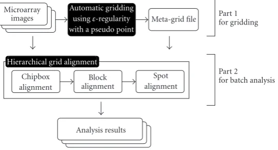
is a hierarchical metagrid alignment methodology to provide reliable and efficient batch processing for a set of microarray images.Figure 2shows a flow chart of our automated im-age analysis system. The basic idea of our automatic gridding algorithm is as follows. In a microarray image, if the spots are in a single block, it is highly likely that they are in the form of a regular sequence. So we compute a set of regular sequences for an entire microarray image and then cluster the “near” regular point patterns, which form a spot grid in a single block. However, handling microarray images with a low expression rate and/or experimental error is difficult. Our model easily overcomes this problem. In batch process-ing, we align the metagrid to a real image according to the structure of the metagrid which consists of a chipbox, blocks, and spots.
The organization for this paper is as follows.Section 2 ex-plains the concept of the extendedδ-regular point sequence and how to apply this procedure to locate the block/spot in-dex. Hierarchical metagrid alignment will be discussed in Section 3. Finally, experimental work and results are given in Sections4and5.
2. EXTENDEDδ-REGULAR SEQUENCE
The task of detecting regular spatial sequences in images arises in many computer vision applications, including scene analysis, military applications, and other areas [9, 10]. The general problem is one of recognizing equally spaced collinear subsets in a given set of points. In an ideal microar-ray image, all of the spots in a row or column in each block should be included in the exact regular sequence. However, it is not desirable to apply an ideal definition of regular pat-tern sequence to a microarray image, since a microarray im-age contains much noise and the location of each spot varies somewhat in practice due to the mechanical error in the mi-croarray production machine (spotter). So we propose a new
relaxedalgorithm to compute the regular sequences and to
correctly locate the positions of spots and blocks.
2.1. Preliminary
In the ideal microarray image, all spots in a row/column are collinear and equally spaced. So we give formal definitions of “collinear” and “equally spaced” for the given finite set of points.
Definition 1. P= {p1,p2,. . .,pn}is calledcollinearif the area (pi,pj,pk) = 0 and|P| ≥ 3. In a similar way,P = {p1, p2,. . .,pn}is calledequally spacedif|pi−pi−1| = |pi+1−pi|,
for 2 ≤i ≤ n−1. Note that|p−q|denotes the Euclidian distance between pointspandq.
Now, we define a regular sequence as follows.
Definition 2. P = {p1,p2,. . .,pn}is aregular point sequence
ifPis collinear and equally spaced.
A maximal regular sequence of a set of points is one that is not properly contained as a contiguous subsequence in any other regular sequence. Based on the definition of a regular sequence, we define theδ-regular sequence as follows.
Definition 3. A sequence of points isδ-regular if each of its points can be displaced by at mostδalong each axis to yield a regular sequence; that is, given a fixedδ ≥0, a sequence of pointsP= {p1,p2,. . .,pn} ⊂E2is aδ-regular sequenceif P = {p1,p2,. . .,pn}andδ≥ |xi−xi|,δ ≥ |yi−yi|, for all
1≤i≤n, wherepi=(xi,yi) andpi=(xi,yi) [10].
Definition 4. Amaximalδ-regular sequenceis one that is not properly contained as a contiguous subsequence in any other δ-regular sequence.
A regular sequence should be one of aδ-regular sequence with δ = 0. Figure 3 shows an example of a maximalδ -regular sequence. In order to show a more relaxed form of a regular sequence, we define anextendedδ-regular sequence for analyzing microarray images.
Definition 5. A set of δ-regular sequences is called an
ex-tendedδ-regular sequence if we can make them a singleδ
-regular sequence by adding pseudopoints in between them.
Figure 4shows how to construct extendedδ-regular se-quences from input points. Simply, the extendedδ-regular sequence is constructed by concatenating two adjacent and collinearδ-regular sequences by inserting pseudopoints be-tween them.
2.2. Automatic block indexing
A maximalδ-regular sequence helps calculate the rotational angleθ and unit distance duof a given microarray image,
Microarray images
Automatic gridding usingε-regularity with a pseudo point
Meta-grid file
Hierarchical grid alignment
Chipbox alignment
Block alignment
Spot alignment
Analysis results
Part 1 for gridding
Part 2
for batch analysis
Figure2: A flow chart of our automatic image analysis system. Part 1 is responsible for performing automatic gridding by using the extended
δ-regular sequence and part 2 aligns the metagrid to the images using hierarchical metagrid alignment for batch processing.
2ε
2ε
Figure 3: A δ-regular sequence: a sequence (solid dots) whose
points are withinδof the corresponding (ideal) points of a regu-lar sequence [10].
In our method, we first construct a set of points{Pi}by image segmentation and by computing the geometric cen-ter of the spots. From this, we will find maximalδ-regular sequences. Let stepi denote the distance between adjacent
points in a δ-regular sequence ri. Algorithm 1 shows the
method for calculating the rotational angle and the unit dis-tance. InAlgorithm 1, we use the spots detected by segmenta-tion methods, and then we perform spot filtering to remove spurious spots. A set of spots may contain several spurious spots after filtering. However, since the probability of the maximal occurrence of aδ-regular sequence which is com-posed of spurious spots is very low, they are not generally considered. In extreme cases, some spurious spots may not be eliminated by our algorithm, but every automated image analysis system fails to provide for some type of some ex-treme case. Handling spurious spots is an important aspect of the process. However, previous systems have not consis-tently responded to these spots.
Next, we generate a block of{Pi}with rotational angle,θ, and unit distance,du.Algorithm 2shows the steps for block
construction.Figure 5shows anextendedδ-regular sequence in a microarray image. Figure 5(a) shows the input point set,Figure 5(b)is theδ-regular sequences ofFigure 5(a), and Figure 5(c)is theextendedδ-regular sequence.
Let the number of expressed spots ben and the valid cells bem. The work of Andrew implies anΘ(n2) time
algo-rithm for all maximal regular sequences in two dimensions [9]. We calculate all of the maximal regular sequences of a set of points ofvalid cellsto get the rotational angle and unit distance of the microarray image.
3. HIERARCHICAL METAGRID ALIGNMENT
Since the date of a single microarray experiment consists of 10∼20 scanned images obtained from an identical microar-ray, the grid structure computed for the first image can be applied to all of the following images (especially for the du-plicate experiment data). So it is reasonable to use batch pro-cessing for the scanned images obtained from an identical chip. Therefore most commercial systems (such as GenePix [11] and ImaGene [12]) provide a metagrid file to enable batch processing. A metagrid file is a template file that con-tains the properties (e.g., dimension, location, size, etc.) of the blocks and spots in a microarray image. Without a meta-grid file, an experiment must find the spot/block index for every raw microarray image one by one. Batch processing with a metagrid proceeds as follows.
(1) Generate a metagrid template based on a base microar-ray image.
(2) Load one raw image file and a ready-made metagrid template.
(3) Compute the signal intensity of the image segmenta-tion bounded by a metagrid circle for a spot.
It should be noted that the geometric properties (the physical locations of the blocks and spots) of a scanned image differ slightly from each other although they have all been obtained from the same microarray slide. This is due to the mechani-cal errors of scanners and experimental (manual work) error. Figure 7shows the result of metagridding using an identical GAL file (a metagrid file provided in GenePix).Figure 7(b) shows a typical case of metagrid displacement. Clearly, the metagridding method requires some manual work.
In this section, we propose a new algorithm,hierarchical
metagrid alignment(HMA). HMA consists of three
sequen-tial steps: chipbox, block, and spot alignments. The problem of aligning a metagrid to a given image could be considered as a point set matching problem [13]. But it is an expensive algorithm, running inO(n3) (nis point number). Applying
(a)
s1
s2
(b)
s1
s2 s3
s4
(c)
s1
s5 s3
(d)
Figure4: (a) Input points, (b) regular sequences, (c)δ-regular sequences, (d) extendedδ-regular sequences. An empty circle denotes an
inserted pseudopoint.
Input: (i){Pi}; a set of center points of expressed spots (ii)δ; a threshold constant given by user.
Output: rotational angleθand unit distancedu.
(1) Divide a microarray image into cells whose sizes are 2∗δ
by 2∗δfor the givenδ-value.
Letcv(valid cell) refer to a cell that contains at least one spot ofP.
(2) Construct a set of center pointsPofcvsand compute all maximalδ-regular sequencesR= {r1,r2,. . .,rn}ofP. Figure 6shows an example ofvalid cell,Pi, and center
points ofvalid cells.
We construct only therithat havestepismaller than the
stepj(1≤j≤i−1). Ifstepi=2·δ, we selectriand exit this procedure.
(3) Select maximalδ-regular sequencesRwhich has the smallest step.
(4) Setθ=the angle ofRto horizontal line,
du=distance between the adjacent points in theR.
Algorithm1: Computing the rotational angle of a given image and
the unit distance between two adjacent spots.
3.1. Chipbox alignment
Let ChipBox be the minimum rectangular area including
all blocks in a chip. There are two kinds of chipboxes: one
ismChipBox from the metagrid, and the other isfChipBox
fromfSpots(the real image given). In the following,mBlock
(mSpot) denotes the block (spot) of a metagrid and
simi-larly,fBlock(fSpot) denotes the block (spot) of a scanned im-age. TheChipBox alignment is to determine thefChipBox,
somChipBoxis aligned withfChipBoxby matching the left
upper points of the two regions. We first determine the
fChipBox to calculate MBR of all expressed spots and then
align themChipBoxwith thefChipBox.
Figures8(a)and8(b)show the before/after snapshots of the chipbox alignment. In Figures8(a)and8(b), the yellow objects indicate target spots, the red rectangle is afChipBox and the cyan objects aremBlocks.
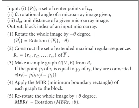
Input: (i){Pi}; a set of center points ofcv,
(ii)θ; rotational angle of a microarray image given, (iii)du; unit distance of a given microarray image. Output: block index of an input microarray. (1) Rotate the whole image by−θdegree.
{Pi} =Rotation ({Pi},−θ).
(2) Construct the set of extended maximal regular sequences
Re= {re1,re2,. . .,ren}ofP
.
(3) Make a simple graphG(V,E) fromRe.
If the pointpiofriis equal topjofrj, they are connected.
e(vi(≡pi),vj(≡pj)).
(4) Apply the MBR (minimum boundary rectangle) of each graph to the block.
(5) Re-rotate the whole image by +θdegree.
MBRs=Rotation (MBRs, +θ).
Algorithm2: Block gridding.
3.2. Block alignment
Assume that the chipbox alignment has already been per-formed.Figure 9(a)shows a situation in which themBlock does not correctly match thefBlock. So we have to align ev-ery block. Block alignment is similar to chipbox alignment. First, we divide the chipbox intouBlocksfor detectingfBlocks using the gap between the nearest blocks and the block size from metagrid. Second, we assign the fBlocks to MBR of expressed spots in theuBlocksand then align thefBlockswith themBlocks. We perform the following two steps to align the mBlockswith thefBlocks.
(1) We align the fBlocks which are similar in size to mBlocks. In this case, we align thefBlockto fitmSpot0,0,
which is the upper left spot in themBlock, with the up-per left position of the fBlock.
(a) (b)
(c) (d)
Figure5: A simple example of a grid structure constructed from an
extendedδ-regular sequence with input points: (a) input points, (b) a graph byδ-regular sequence merging, (c) adding pseudopoints betweenδ-regular sequences, (d) a grid graph by merging all ex-tendedδ-regular sequences. The shaded box points are the inserted pseudopoints.
(1, 1)
Pj
cv
Pi
δ
(3, 3)
Figure6: An example of{Pi}, valid cells and center points of valid
cells. We construct a set of center pointsP ofcv (valid cell)s and compute all maximalδ-regular sequencesR= {r1,r2,. . .,rn}ofP.
Figure 9shows the before/after snapshots of the block alignment. The red rectangle denotes thefBlockand the cyan objects denote themBlock.
3.3. Spot alignment
This step assumes that the chipbox and the block are already aligned. Now we want to align the metagrid spot (mSpot) to the real grid spot (fSpot). The spot alignment in each block
(a) ImageIa
(b) ImageIb
Figure 7: The metagridding snapshots of two images using the
same GAL file in GenePix.Iashows that the metagrid fits the given image correctly.Ibshows an image that has a discrepancy between the metagrid and the given image. Manual work is required forIb.
is the last step of HMA. In this alignment, we first have to classifymSpotsintoactive spotsandnonactive spots.Figure 10 shows an active spot and a nonactive spot. AmSpot is an active spot if it has one fSpot within the distance,d. After identifying all active spots, we align theactive spotsto the cor-respondingfSpots.
Figure 11shows the result of spot alignment. InFigure 11(b), the red circles denoteactive spotsand the cyan objects arenonactive spots.
4. EFFECTIVENESS OF EXTENDED
δ-REGULAR SEQUENCE
Generally, the length (the number of points) of an extended δ-regular sequence is expected to be longer than that of aδ -regular sequence. First, we need to know the expected size of theextendedδ-regular sequenceand theδ-regular sequence.
LetPδdenote the probability that there exists at least one
(a)
(b)
Figure8: (a) A snapshot before chipbox alignment, (b) a snapshot
after chipbox alignment. The yellow object is afSpot, the red rect-angle is afChipBox, and the cyan object is amBlock.
probability,Pδ, is given as follows:
Pδ=Prob(boundaryδ−regular sequence)
+ Prob(middleδ−regular sequence)
= n−2
i=3
(s·q)i(1−s·q) +
n−1
i=3
(s·q)i(1−s·q)2
=(s·q)3(1−s·q)
×
1−(s·q)n−4+ (1−s·q)1−(s·q)n−3
(1−s·q) . (1)
LetPE be the probability that there exists at least one
extended δ-regular sequence of length i inS. An extended δ-regular sequence includes two types of sequences: one from the original δ-regular sequence and another from the concatenation of two adjacent δ-regular sequences by adding one pseudopoint in the middle of those twoδ-regular sequences. SoPEshould be
PE=Pδ+ Prob(δ−regular sequence extends)
=Pδ+
n−2
i=3
(s·q)i−1(1−s·q)3+ n−1
i=3
(s·q)i−1(1−s·q)2
(a) A snapshot before block alignment
(b) A snapshot after block alignment
Figure9: (a) A snapshot before block alignment, (b) a snapshot
af-ter block alignment. In (a) and (b), the red rectangle denotes the fBlockand the cyan (yellow) object denotesmSpot(fSpot), respec-tively.
=Pδ+ (s·q)2(1−s·q)2
×(1−s·q)
1−(s·q)n−5+1−(s·q)n−4
(1−s·q) . (2)
We compute the expected length of the δ-regular se-quence and the extendedδ-regular sequence inSwith|S| =
n,E(Lδ)=
n
k=3k·Pδ, andE(LE)=
n
k=3k·PE.
This calculation reveals the effectiveness of the “ex-tended” δ-regular sequence versus the δ-regular sequence. The calculation shows that the extendedδ-regular sequence is more than twice the length of theδ-regular sequence if the spot expression rate is low (seeTable 1andFigure 12). If the expression rate is high, there is no difference. This means that if the expression rate, s, and tolerance probability, q, approach 1, the extendedδ-regular sequence should be the same as theδ-regular sequence.
mspot Active spot
fspot
d
(a)
mspot Nonactive spot
fspot
d
(b)
Figure10: AmSpotis an active spot if it has onefSpotwithin
dis-tance,d. (a) An active spot, (b) a nonactive spot.
(a)
(b)
Figure11: The progress ofspot alignment. (a) A snapshot of active
spots, (b) a snapshot after spot alignment. The red circles and cyan objects denoteactive spotsandnonactive spots, respectively.
We have shown that aδ-regular sequence can be exten-ded to another longerδ-regular sequence by inserting one pseudopoint in between two disjoint and collinearδ-regular sequences. Now we will show the effectiveness of this ex-tendedδ-regular sequence for the spot indexing procedure.
LetPa be a set of points obtained by spot image
seg-mentation for a microarray image. As we explained above, we construct a geometric grid graph G(Pa) after spot
seg-mentation by adding edges among them.Figure 13shows an
Table1: Comparison of the expected length of the extendedδ
-regular sequence (=E(LE)) and the expected length of theδ-regular sequence (= E(Lδ)), where the number of point rows (n = 20), columns (n=20), andq=0.9.
s·q E(Lδ) E(LE) E(LE)/E(Lδ)
0.40 1.06 2.7 2.50 0.45 1.26 2.82 2.22 0.50 1.49 3.00 2.00 0.55 1.77 3.22 1.81 0.60 2.10 3.50 1.67 0.65 2.50 3.85 1.54 0.70 3.02 4.32 1.43 0.75 3.72 4.96 1.33 0.80 4.69 5.86 1.25 0.85 6.13 7.21 1.18 0.90 8.42 9.37 1.11 0.95 12.42 13.08 1.05 1.00 20.00 20.00 1.00
0.4 0.45 0.5 0.55 0.6 0.65 0.7 0.75 0.8 0.85 0.9 0.95 1 1
1.2 1.4 1.6 1.8 2 2.2 2.4 2.6
sq
E(LE)/E(Lδ)
Figure12:E(LE)/E(Lδ), the ratio of the expected length of the
ex-tendedδ-regular sequence to theδ-regular sequence.
example for segmented spots and its correspondingG(Pa). If
G(Pa) is connected and the minimum bounding box (MBR)
ofG(Pa) is the same as to the MBR of a single block of
mi-croarray image given, then we callG(Pa) successful since we
correctly separate each block in the whole microarray image. It is crucial to get a successfulG(Pa), which enables us to
in-dex (i,j) of each spot automatically. Otherwise, if G(Pa) is
disconnected or MBR of G(Pa) does not cover a block
re-gion, thenG(Pa) is called unsuccessful for the given
microar-ray image since we do not automatically index the spots. LetGδ(Pa) (Geδ(Pa)) be a grid graph obtained from a
set of δ-regular sequences (extended δ-regular sequences). Figure 14(b)shows an unsuccessful example ofGδ(Pa) and
Figure 14(d)shows a successful example ofGeδ(Pa). In order
to give the spot index of an unsuccessfulGδ, manual
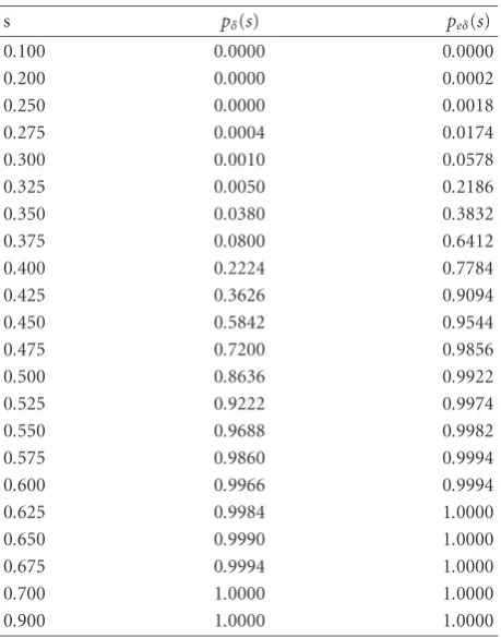
Table2: Probability functionspδ(s) andpeδ(s).
s pδ(s) peδ(s)
0.100 0.0000 0.0000
0.200 0.0000 0.0002
0.250 0.0000 0.0018
0.275 0.0004 0.0174
0.300 0.0010 0.0578
0.325 0.0050 0.2186
0.350 0.0380 0.3832
0.375 0.0800 0.6412
0.400 0.2224 0.7784
0.425 0.3626 0.9094
0.450 0.5842 0.9544
0.475 0.7200 0.9856
0.500 0.8636 0.9922
0.525 0.9222 0.9974
0.550 0.9688 0.9982
0.575 0.9860 0.9994
0.600 0.9966 0.9994
0.625 0.9984 1.0000
0.650 0.9990 1.0000
0.675 0.9994 1.0000
0.700 1.0000 1.0000
0.900 1.0000 1.0000
Letpδ(s) and peδ(s) be the probability functions of the
expression rate s that grid graphs Gδ(Pa) andGeδ(Pa) are
successful, respectively. Now we want to compare the prob-abilities pδ(s) and peδ(s). Since the expression rate of each
spot is a random variable,G(Pa) should be a kind of a
ran-dom graph where the existence of each edge is dependent on a probabilistic model.
There are so many interesting results on random graph [14]. One of interesting results is about the characteristics in the probability of graph connectedness. That is the fa-mous Erd¨os and Renyi theorem [15]. Letpbe the probability of edge existence with n vertices graph. It is known that p =logn/nis the threshold function for graph connected-ness. That means if limp/(logn/n)=0 implies limpδ(s)=0
and if limp/(logn/n)=1 implies limpeδ(s)=1, this
thresh-old function property is one important feature of random graph.
So far we did not find any probabilistic graph model which is exactly the same as microarray grid graphs. We be-lieve that constructing a rigorous probabilistic model for this grid graph is very hard. Instead of this, we tried to apply a Monte-Carlo method to estimate the threshold value for the connectedness of random grid graph by using 50 000 artifi-cial grid graphs.
First we generate 50 000 sets of artificial spot to sim-ulate microarray images for each expression rate s = 0.1, 0.2,. . ., 0.7, 0.9. LetPU be the set of 50 000 point sets. Next
we constructGδ(Ps) andGeδ(Ps), for eachPs∈PU.
(a)
G(Ps) MBR
(b)
Figure13: (a) A set of spot points,Pa, obtained from a
microar-ray image segmentation. (b) A case of unsuccessfulG(Pa) since the MBR ofG(Pa) does not cover the whole block.
(a) (b)
(c) (d)
Figure14: Example for unsuccessful and successful cases where
ex-pression rates=0.51. (a) A set of input points,Pa. (b) A case of un-successfulGδ(Pa), due to 7 disconnected components. (c) A point setPb=Pa∪ {pseudopoints inserted}. Each “◦” denotes a pseudo-point. (d) SuccessfulGeδ(Pa), which is one connected component and its MBR covers the whole block.
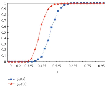
Table 2shows thepδ(s) andpeδ(s) values andFigure 15
shows pδ(s) and peδ(s) curves according to the expression
rates. InFigure 15, solid curve and dotted curve denotepδ(s)
andpeδ(s), respectively. As was noted, we can see the sharp
hill of the threshold value for graph connectedness. Interest-ingly, we can see that our extended regular sequence gives the much higher successful probability ofGeδ(Ps) in expression
rate intervals[0.3, 0.5] compared toGδ(Ps).
It is also interesting to see that there is no difference be-tweenpδ(s) andpeδ(s), if the spot expression rate is less than
our extendedδ-regular sequence is very helpful and eff ec-tive to enable the automatic spot indexing. The ratio rs =
pδ(s)/peδ(s) is plotted inFigure 16.
Determining the number of pseudopoints to be inserted in aδ-regular sequence is crucial to the gridding of the whole microarray index. The more pseudopoints are allowed, the higher the probability of connectedness for a single block be-comes. But this leads to an undesirable situation in which two adjacent blocks are connected into a single component, which prevents identification of the block structure. There-fore, the number of pseudopoints must be based on the dis-tance between blocks in a scanned real microarray image.
5. EXPERIMENTAL RESULTS
We tested our method using images of four different chips (from a medical center, a university, and a biocompany). Table 3shows the specifications of the test data set. #B and #S are the dimensions of the block and the spot of a given chip, respectively, anddsis the diameter of the spot. gapband
gaps are the gap distances of adjacent blocks and spots, re-spectively. # Img indicates the number of images to be tested per chip.
Figure 17shows the three different grid structures after adjusting the ratiorx=gapb/(2·gaps+ds). This figure shows
thatrxis an important characteristic constant in obtaining a
successful block/spot gridding. It is the samerx =0.5 as the
distance between adjacent center points of expressed spots in the ideal microarray image. InFigure 17,rx=0.25 is too
small to detect each single block andrx = 1.0 is too large
resulting in merged blocks. Optimal block gridding occurs whenrx =0.5. This implies that the block gridding
perfor-mance goes best when the distance between points in both sides of the pseudopoint in an extendedδ-regular sequence.
Figure 18shows an successful gridding result of microar-ray with 2×2 grid structures using our automatic gridding. InFigure 18, microarray image leans about 2 degrees. Our algorithm finds successfully the locations of all blocks and spots.
Now we will explain the efficacy of HMA. Let ΔM de-note the total displacement distance of all spots to metagrid-ding spots. And letΔH denote the total displacement dis-tance needed for HMA.ΔMandΔHare computed as
ΔM=
b∈blocks
i,j∈spots m(b)
i j −s (b)
i j , (3)
wherem(i jb)is the physical position of a metagrid spot whose
index is (i,j) in blockb, and wheres(i jb)is the physical position
of a real spot in the block in a scanned image.
ΔH=ΔChipBox +
b∈blocks
ΔBlockb
+
b∈blocks
i,j∈spots m(b)
i j −s (b) i j ,
(4)
wherem(i jb)is the physical position of a metagrid spot after
chipbox and block alignments. ΔChipBox and ΔBlock are
0 0.2 0.325 0.425 0.525 0.625 0.75 0.95 0
0.1 0.2 0.3 0.4 0.5 0.6 0.7 0.8 0.9 1
s pδ(s)
peδ(s)
Figure15: The probability functionspδ(s) andpeδ(s) according to
the expression rates. Solid and dotted curves denote thepδ(s) and
peδ(s), respectively.
0 0.3 0.35 0.4 0.45 0.5 0.55 0.6 0.65 0.7 0.8 0.9 0
10 20 30 40 50 60 70
pδ(s)/ peδ(s)
s
Figure16: The ratiors=Pδ(s)/Peδ(s) with respect to the expression
rates(horizontal axis). Ifsis near 0.3, thePeδ(s) is 60 times higher thanPδ(s). Ifs=0.325, thersis about 40.
Table3: The specification of the test data set.
Chip #B #S ds gapb gaps # Img A 4×4 12×14 14 98.58 12.20 5 B 4×4 10×10 16 90.75 18.90 8 C 4×4 18×18 14 34.13 8.53 8 D 4×4 10×10 16 91.66 18.81 8
the displacement distances of the chipbox and block align-ments, respectively. Figure 19 compares the ΔM and ΔH, which were computed with four chips using HMA, and a straightforward metagrid overlapping. We can see that HMA drastically reduces the displacement distance by more than 90% as compared to the straightforward simple metagrid-ding.
(a)rx=0.25
(b)rx=0.5
(c)rx=1.0
Figure17:rxand its corresponding autogridding result in chip B.
(a)rx=0.25 does not detect the block clusters. (b)rx =1.0 is too large resulting in merged blocks. (c)rx=0.5 gives the optimal block gridding.
the metagridding results before HMA (none) have many dis-placement distances, but the further the alignment processes in HMA proceed, the better the results are. HMA finally at-tains the ideal gridding results.
6. CONCLUSION
It is very important to develop an automated and intelligent system for analyzing microarray images. The contributions of this paper are as follows.
Figure18: The correct gridding result. This image consists of 4×4
blocks with 18×18 spots each, and leans about 2 degrees.
Chip A Chip B Chip C Chip D
0 2 4 6 8 10 12 14
×104
The
displac
ement
distanc
e
Metagridding
Hierarchical metagrid alignment
Figure19: Total displacement distance required by metagridding
and our HMA.
None Chipbox Block Spot
0 10 20 30 40 50 60 70 80
T
o
tal
displac
ement
distanc
e
betw
een
real
spots
and
m
etag
ri
d
Chip A Chip B
Chip C Chip D Alignment step
Figure 20: Reduction of displacement distances after {chipbox,
box, spot}alignment.
(ii) HMA (hierarchical metagrid alignment) is a novel method for processing microarray image batches be-tween all real spots and metagrid spots, and reduces the total displacement distance by more than 90% as compared to straightforward metagridding methods (e.g., GenePix style).
We are developing a more rigid probabilistic model for the extended δ-regular sequence. It is well known that the probability of connectedness for a random graph approaches 1 when the edge probability of the random graph is above O(logn/n). It is easy to see that the graph model con-structed from the microarray point sequences for block/spot indexing is a bipartite graph. So it is instructive to deter-mine the probability of bipartite graph connectedness when the edge probability, p, is given. We also use Monte-Carlo simulation method to estimate the probability of the con-nectedness of the grid graph. It is also a very interest-ing problem to establish the complete probabilistic model for the grid graph obtained from microarray experiment. The supplemental information is available on our website (http://jade.cs.pusan.ac.kr/∼gridding).
ACKNOWLEDGMENTS
This research was supported by a Grant (M10529000001-05N2900-00110) from Strategic National R&D Program of Ministry of Science and Technology. We gratefully credit the thoughtful reviewers who provided substantial constructive criticism on an earlier version of this paper.
REFERENCES
[1] D. J. Duggan, M. L. Bittner, Y. Chen, P. Meltzer, and J. M. Trent, “Expression profiling using cDNA microarrays,”Nature genet-ics, vol. 21, pp. 10–14, 1999.
[2] D. Shalon, S. J. Smith, and P. O. Brown, “A DNA microarray system for analyzing complex DNA samples using two-color fluorescent probe hybridization,” Genome Research, vol. 6, no. 7, pp. 639–645, 1996.
[3] A. A. Alizadeh, M. B. Eisen, R. E. Davis, et al., “Distinct types of diffuse large B-cell lymphoma identified by gene expression profiling,”Nature, vol. 403, no. 6769, pp. 503–511, 2000. [4] M. Steinfath, W. Wruck, H. Seidel, H. Lehrach, U. Radelof, and
J. O’Brien, “Automated image analysis for array hybridization experiments,”Bioinformatics, vol. 17, no. 7, pp. 634–641, 2001. [5] R. Hirata Jr., J. Barrera, R. F. Hashimoto, and D. O. Dan-tas, “Microarray gridding by mathematical morphology,” in Proceedings of 14th Brazilian Symposium on Computer Graph-ics and Image Processing (SIBGRAPI ’01), pp. 112–119, Flo-rian ´opolis, Brazil, October 2001.
[6] H.-Y. Jung and H.-G. Cho, “An automatic block and spot in-dexing withk-nearest neighbors graph for microarray image analysis,”Bioinformatics, vol. 18, no. suppl 2, pp. S141–S151, 2002.
[7] G. Kauer and H. Bl¨ocker, “Analysis of disturbed images,” Bi-oinformatics, vol. 20, no. 9, pp. 1381–1387, 2004.
[8] T. Srinark and C. Kambhamettu, “A microarray image analysis system based on multiple-snake,”Journal of Biological Systems Special Issue, vol. 12, no. 4, pp. 202–209, 2004.
[9] A. B. Kahng and G. Robins, “Optimal algorithms for extract-ing spatial regularity in images,”Pattern Recognition Letters, vol. 12, no. 12, pp. 757–764, 1991.
[10] G. Robins, B. L. Robinson, and B. S. Sethi, “On detecting spa-tial regularity in noisy images,”Information Processing Letters, vol. 69, no. 4, pp. 189–195, 1999.
[11] GenePix,http://www.axon.com.
[12] ImaGene,http://www.biodiscovery.com/imagene.asp. [13] T. S. Caetano, T. Caelli, and D. A. C. Barone, “An optimal
probabilistic graphical model for point set matching,” in Pro-ceedings of Joint IAPR International Workshops on Structural, Syntactic, and Statistical Pattern Recognition (S+SSPR ’04), pp. 162–170, Lisbon, Portugal, August 2004.
[14] J. Spencer, Ten Lectures on the Probabilistic Method, SIAM, Philadelphia, Pa, USA, 1990.
[15] B. Bollob´as, Random Graphs, Cambridge University Press, Cambridge, UK, 2001.
Hee-Jeong Jinreceived her B.S. degree in 2000 from Pusan National University, South Korea, the M.S. degree in 2002 from Pu-san National University, South Korea. From 2002 to 2003, she had been in National Genome Research Institute, KNIH, and since 2003, she has been a Ph.D. candidate in Pusan National University, South Ko-rea. Her research interest is bioinformatics (analysis of ppi, comparative genomics, and microarray gridding).
Bong-Kyung Chun received his B.S. de-gree in 2003 from Pusan National Univer-sity, South Korea, the M.S. degree in 2005 from Pusan National University, South Ko-rea, and since 2005 he has been a Ph.D. stu-dent in Pusan National University, South Korea. His research interests are bioinfor-matics and computer graphics.
Hwan-Gue Choreceived his B.S. degree in 1984 form Seoul National University, South Korea, the M.S. degree in 1986 from Ko-rea Advanced Institute of Science and Tech-nology, South Korea, and the Ph.D. in 1990 from Korea Advanced Institute of Science and Technology, South Korea. Since 1990 he has been a Professor in Pusan National University, South Korea. His research inter-ests are graphics (visualization) and
![Figure 1: A typical raw image of a microarray: it consists of 4blocks and each block is composed of 24 × 4 × 24 spots [3].](https://thumb-us.123doks.com/thumbv2/123dok_us/1150463.1144450/2.600.89.258.73.240/figure-typical-image-microarray-consists-blocks-block-composed.webp)