Volume 2009, Article ID 426589,17pages doi:10.1155/2009/426589
Research Article
Target Localization by Resolving the Time
Synchronization Problem in Bistatic Radar Systems Using
Space Fast-Time Adaptive Processor
D. Madurasinghe and A. P. Shaw
Electronic Warfare and Radar Division, Defence Science and Technology Organisation, P.O. Box 1600, Edinburgh, SA 5111, Australia
Correspondence should be addressed to D. Madurasinghe,[email protected]
Received 30 September 2008; Accepted 26 January 2009
Recommended by Magnus Jansson
The proposed technique allows the radar receiver to accurately estimate the range of a large number of targets using a transmitter of opportunity as long as the location of the transmitter is known. The technique does not depend on the use of communication satellites or GPS systems, instead it relies on the availability of the direct transmit copy of the signal from the transmitter and the reflected paths offthe various targets. An array-based space-fast time adaptive processor is implemented in order to estimate the path difference between the direct signal and the delayed signal, which bounces offthe target. This procedure allows us to estimate the target distance as well as bearing.
Copyright © 2009 D. Madurasinghe and A. P. Shaw. This is an open access article distributed under the Creative Commons Attribution License, which permits unrestricted use, distribution, and reproduction in any medium, provided the original work is properly cited.
1. Introduction
Bistatic radar systems are gaining more and more interest over the past two decades due to the freedom and flexibility it offers in deploying transmitters and receivers. Other advan-tages include the ability to use inexpensive receive modules, the use of continuous wave signals, the use of transmitters of opportunity, lower maintenance cost, operation without frequency clearance (if using third party transmitters), covert operation of the receiver, increase resilience to electrometric countermeasures, ability to hide the receiver location and the waveform being used, and huge enhancement of the target radar cross-section due to geometrical effects. However, several disadvantages include the system complexity, cost of providing communication between sites, lack of any control over the transmitter (if using third party transmitters), and reduced low-level coverage due to the need for line-of-sight from several locations.
Passive radar systems (also referred to as passive coherent location and passive covert radar) encompass a class of radar systems that detect and track objects by processing reflections from noncooperative sources of illumination in the environment, such as commercial broadcast and
communications signals. It is a specific case of bistatic radar that exploites cooperative and noncooperative radar transmitters. References [1–5] are some of the examples.
approaches include the use of GPS systems that may allow us to synchronize the time over a reasonably long period with a time difference of less than 1 nanosecond. This topic has been discussed widely in the existing literature by various authors and various improved methods are also available. References [6–9] are some of the examples. In this study we propose an innovative approach to locate the targets without the aid of the communication satellites or the GPS systems. Under the proposed technique, one does not need to maintain any form of synchronization between transmitter and receiver, in respect of, instant of pulse transmission and transmit signal phase.
This study introduces a technique to resolve the synchro-nization problem related to bistatic radar by using a new and emerging class of signal processing technique that may be referred to as space fast-time adaptive processing (SFTAP). The SFTAP is conventionally applied to null mainlobe interferers using an array of receivers in a monostatic configuration [10–15]. In a conventional space fast-time adaptive processor one blindly stacks a large number of consecutive range cell returns to form a space fast-time adaptive processor expecting that the process would null the interference signal (commonly known as the mainlobe signal) due to the presence of its delayed copies known as terrain scattered interference paths. Recent advances in this type of signal processing have led to the introduction of a processor known as the Terrain Scattered Interference (TSI) finder [14], the function of which is to avoid the stacking of a large number of range cells blindly, instead it leads the SFTAP processor to the correct range cell position to form the space fast-time data snap. The TSI finder basically identifies all the delayed copies of the signal of interest, which include the multipath bounces offvarious other targets and the ground. This is achieved by forming a space fast-time beam in the direction of the signal of interest, or in our case the transmitter, by assuming the bearing of the transmitter is precisely known. Such a beam is able to null all other existing sidelobe arrivals, which are known as interferers or jammers, which are uncorrelated with the signal of interest. The objective of the beam is to identify all the sidelobe arrivals which are delayed versions of the look direction signal.
An application of this theory would be the detection of airborne targets in a maritime environment where the transmitter is placed several kilometers away from the maritime platform in a known position (or the position of a moving transmitter location is accurately known to the receiver system in order to form the space-time beam at any given time). Another important application would be to detect high altitude or space-based targets, such as intercontinental ballistic missiles, using a bistatic arrange-ment where a series of transmitters and receivers can be geographically distributed to achieve the best possible results. In such a scenario, one would locate all the transmitters in high altitude locations (mountains), where receivers can receive direct signal (which can be a random continuous waveform) from all or most of the transmitters in order to track each of the multipath signals (target reflections) originating due to the known transmitters. The proposed
z y x
γ
d s1
s2
φ
−θ
Ground Target
Array
Interfer enc
e (jammer) Multipathx( t−
τ2)
Direct (source) signal
x(t) M
ultipath
x( t−
τ1)
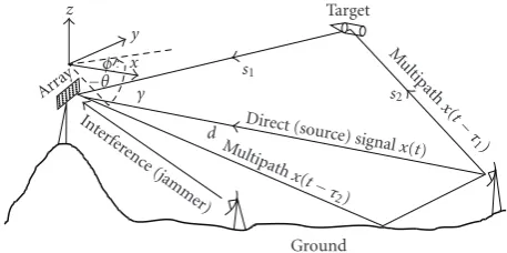
Figure1: Transmitter and receiver arrangements with an airborne target, a jammer, and one transmitter.
algorithm will identify each multipath with its associated direct transmit signal, by forming a space fast-time beam in the direction of each known transmitter.
We aim to solve the problem by locking the radar receiver in the direction of a known transmitter at a known bearing and distance (usually a third party transmitter in the line-of-sight). The objective is to receive its direct signal by forming a beam in the direction of the transmitter (a space-time beam), which allows us to effectively form a secondary search beam for arrival of the same stream of data (with a delay) due to reflections off the targets and the ground (these beams are formed simultaneously). Such delayed versions usually have a different bearing and a fixed delay factor during the integration period. In this study these are termed as multipath arrivals of the main beam signal (or in the case of ground reflections they are termed as TSI arrivals). Once this knowledge is established, for every multipath or TSI arrival, one can estimate the location of the reflection point via triangulation. While some points are identified as targets some may correspond to ground reflections. Reflection points which vary over time may be classified as moving targets, at a postprocessing stage.
In this study, first we formulate the problem (Section 2), and then in Section 3 we discuss the properties of the original TSI finder. In Section 4 we introduce the second processor (a postprocessor) to identify all target bearings that may include all the bounced rays off the moving targets as well as stationary targets (ground reflections), by forming a beam in the desired direction which in this case is the transmitter direction. In order to achieve this, we introduce an innovative multipath bearing estimator using two very different optimization approaches. Both solutions are discussed in detail as potential solutions to the multipath bearing estimation problem.Section 5briefly presents the formula for estimating the target location. Finally in Section 6 we carry out a simulation study to demonstrate bistatic scenarios including multiple air target detection using a known transmitter in a known direction, which transmits a random continuous wave signal.
2. Formulation
where φ is the azimuth angle, θ is the elevation angle, s(φ,θ)Hs(φ,θ) = N, and the superscript H denotes the Hermitian transpose. Thetth range gate,N ×1 measured signal x(t) (t is also the fast-time scale or an instant of sampling in fast-time) can be written as
x(t)=j1(t)s
φ1,θ1
+j2(t)s
φ2,θ2
+
a1
m=1
β1,mj1
t−n1,m
sφ1,m,θ1,m
+
a2
m=1
β2,mj2
t−n2,m
sφ2,m,θ2,m
+ε, (1)
where j1(t), j2(t) represent a series of complex random amplitudes corresponding to two far field sources, with the directions of arrival pairs, (φ1,θ1) and (φ2,θ2), respectively. The third term represents Scattered Interference (in our case, multipath bounces) paths off the first source with time lags (path lags) n1,1,n1,2,n1,3,. . .,n1,a1, the scattering
coefficients|β1,m|2 <1,m =1, 2,. . .,a1, and the associated direction of arrival pairs (φ1,m,θ1,m) (m=1, 2,. . .,a1). The fourth term is the multipaths off the second source with path delaysn2,1,n2,2,n2,3,. . .,n2,a2, the scattering coefficients |β2,m|2 < 1,m = 1, 2,. . .,a2, and the associated direction of arrivals (φ2,m,θ2,m) (m = 1, 2,. . .,a2). More sources and multiple paths from each source are accepted in general, but for the sake of brevity, we represent one of each andε represents theN×1 white noise component. In this study we consider the clutter-free case. Furthermore, we assume that ρ2
k = E{|jk(t)|2}(k = 1, 2,. . .) are the power levels
of each source, and|βk,m|2ρ2k (m = 1, 2,. . .) represent the
multipath power levels associated with each bounce from thekth source, whereE{·}denotes the expectation operator with respect to the variable t. Throughout the analysis we assume that we are interested only in the source powers (as potential transmit sources) that are above the channel noise power, that is, snrk = ρ2k/σn2 > 1, k = 1, 2,. . .,
E{εεH} = σ2
nIN, where snrk is the transmit source power
to noise power ratio per channel, σ2
n is the white noise
power present in any channel, and IN is the unit identity
matrix (the effect of snrk = ρk2/σn2 < 1, k = 1, 2,. . .,
is discussed in the simulation section). Without loss of generality we use the notationss1ands2to represents(φ1,θ1) ands(φ2,θ2), respectively, but the steering vectors associated with multipath arrivals are represented by two subscript notations s1,m = s(φ1,m,θ1,m) (m = 1, 2,. . .,a1), s2,m =
s(φ2,m,θ2,m) (m = 1, 2,. . .,a2), and so on. Furthermore it is assumed thatE{jk(t+l)jk(t+m)∗} = ρ2kδ(l−m) (k =
1, 2,. . .), where∗denotes the complex conjugate operation. This last assumption restricts the application of this theory to noise-like sources that are essentially continuous over the period of examination.
3. Multipath Lag Finder
3.1. Multipath Lag versus Power Spectrum. This section looks at a technique that will identify each source (given the source direction) and its associated multipath arrivals (if present).
Here we assume that the radar has been able to identify the desired source as the suitable transmitter (i.e.,ρ2k/σn2>1) and
we would like to identify all its associated multipaths. The formal use of the multipaths (known as Terrain Scattered Interference paths or TSI) is very well known in literature under the topic mainlobe jammer nulling [10–14]. However, the use of the multipath in this study is restricted to the bounces offthe airborne targets (reflections offthe ground are discarded as discussed later). Throughout this study we assume that the first source is our desired transmit source with the known bearing. The array’sN×Nspatial covariance matrix has the following structure (for the case where two sources and one multipath offeach source is present):
Rx=ρ21s1sH1 +ρ22s2sH2 +ρ21β1,1 2
s1,1sH1,1
+ρ22β2,12s2,1sH2,1+σn2IN.
(2)
Suppose now we compute the space fast-time covariance R2 of size 2N×2N corresponding to an arbitrarily chosen fast-time lagn, then we have
R2=E
Xn(t)Xn(t)H
= ⎛
⎝ Rx ON×N ON×N Rx
⎞ ⎠
for n /=n1,m orn2,m m=1, 2,. . .,
(3)
whereXn(t) = (x(t)T,x(t+n)T) T
is termed as the 2N×1 space fast-time snapshot for the selected lag n andON×N
is the N ×N matrix with zero entries. However if n =
n1,m or n2,m for some mthen we have (sayn = n1,1 as an example)
Xn1(t)= ⎛ ⎝ x(t)
xt+n1,1
⎞ ⎠
=j1(t) ⎛ ⎝ s1
β1,1s1,1 ⎞ ⎠+j2(t)
⎛ ⎝ s2
oN×1 ⎞ ⎠
+β1,1j1
t−n1,1 ⎛⎝s1,1
oN×1 ⎞ ⎠+β2,1j2
t−n2,1 ⎛⎝s2,1
oN×1 ⎞ ⎠
+j1
t+n1,1 ⎛⎝oN×1
s1 ⎞
⎠+j2t+n1,1 ⎛ ⎝oN×1
s2 ⎞ ⎠
+β2,1j2
t−n2,1+n1,1 ⎛⎝oN×1
s2,1 ⎞ ⎠+
⎛ ⎝ε1
ε2 ⎞ ⎠,
(4)
whereε1andε2represent two independent measurements of the white noise component, andoN×1is theN×1 column of zeros. In this case the space fast-time covariance matrix is given by
R2= ⎛ ⎝Rx QH
Q Rx
⎞
⎠, (5)
whereQ=ρ2
It is important to note that we assume thatn1,m(m =
1, 2,. . .) represent digitized sample values of the fast-time variabletand the reflected path is an integer-valued delay of the direct path. If this assumption is not satisfied, one would not achieve a perfect decorrelation, resulting in a nonzero off diagonal term in (5) and a clear distinction between (4) and (5) would not be possible. The existence of the delayed value of the termQcan be made equal to zero, or not by suitably choosing a delay value forn when forming the space-time covariance matrix. However,Qis a matrix and as a result one must consider its determinant value in order to differentiate the two cases in (4) and (5). After extensive analysis, one may find the signal processing gain is not acceptable for this choice. A more physically meaningful measure would be to consider its contribution to the overall processor output power (when minimized with respect to the look direction constraint). Depending on whether the power contribution is zero or not we have the situation described in (4) or (5) clearly identified under the above assumptions. The scaled measure was introduced as the TSI finder [14], which is a function of the chosen delay value n, must represent the scaled version of the contribution due to the presence of Q at the total output power. Even though one can come up with many variations of the TSI finder based on the same principle, the one expressed in this study is tested and verified to have high signal processing gain as seen later (the performance degradation of the finder spectrum when the path delay is not an integer multiple of the range resolution is discussed in the simulation section). Now suppose the direction of arrival of the mainlobe source (transmitter) to be (φ1,θ1), the first objective is to find all its associated path delays, which may be of low power. This is carried out by the lag finder in the lag domain by searching over all possible lag values while the look direction is fixed at the desired source direction (φ1,θ1). This is given by the spectrum
Ts(n)=
1
Pout
sH1R−x1s1 −1
, (6)
wherePout=wHR2w,wis the 2N×1 space fast-time weights vector which minimizes the power while looking into the direction of the source of interest (transmitter) subject to the constraints: wHs
A = 1 and wHsB = 0, where sA =
(sT 1,oTN×1, )
T
sB = (oTN×1,sT1) T
. The solution w for each lag is given byw = λR−1
2 sA+μR−21sB, where the parametersλ
andμare given by (one may apply the Lagrange multiplier technique and optimize the function Φ(w) = wHR
2w +
β(wHs
A −1) + ρwHsB with respect to w where β, ρ are
arbitrary parameters. As a result,∂Φ/∂w = 0 gives usw =
λR−21sA+μR−21sB) ⎛ ⎜ ⎝
sH
AR2−1sA sHBR2−1sA
sHAR2−1sB sHBR2−1sB ⎞ ⎟ ⎠ ⎛ ⎝λ∗
μ∗
⎞ ⎠=
⎛ ⎝1
0 ⎞
⎠. (7)
As the search functionTs(n) scans through all potential
lag values, one is able to identify the points at which a corresponding delayed version of the look direction signal (in this example it is the first source) is encountered as seen in the next section.
DenotingRx=ρ21s1sH1 +R1, we have R1=ρ22s2sH2 +β1,1
2
ρ2
1s1,1sH1,1+β2,1 2
ρ2
2s2,1sH2,1+σn2IN.
(8)
(The case of more than two sources and many number of multipaths does not alter the theory to follow, this is discussed in detail inAppendix A).
3.2. Analysis of the Multipath Finder. Now, for the sake of convenience we represent the 2N×1 space fast-time weights vector aswT =(wT
1,w2T) T
, whereN×1 vectorw1refers to the firstNcomponents ofwand the rest is represented byN×1 vectorw2. First suppose that the chosen lagnis not equal to any of the valuesn1,j (j =1, 2,. . .). In this case substituting
(3) andRx=ρ12s1s1H+R1inPout=wHR2wwe have
Pout=w1HR1w1+wH2R1w2+ρ21wH1s1sH1w1+ρ12wH2s1sH1w2. (9)
The minimization of power subject to the same constraints: wHs
A=1 andwHsB=0 (i.e.,w1Hs1=1 andw2Hs1=0) leads to the following solution:
w1= R−1
1 s1 (sH1R−11s1)
, w2=oN×1. (10)
(Note: this procedure cannot be used to find the weights, the earlier described process must be applied to evaluate the space fast-time weights vector).
In this case we have the following expression for the space fast-time processor output power:
Pout=wHR2w =wH
1R1w1+ρ21wH1s1sH1w1 =sH
1R−11s1 −1
+ρ2 1.
(11)
Substituting this expression in (6) leads to
TS(n)n /=n1,1=
sH1R−x1s1 −1
sH1R−11s1 −1
+ρ2 1
−1=0. (12)
(See Appendix B for a proof of the result (sH1R−x1s1)− 1
= (sH1R−11s1)−
1 +ρ2
1). It was noticed that w2 = oN×1 if and only if Q = ON×N. As a result we would consider the
scaled quantityTs(n)=(Pout−wH1R1w1−ρ21wH1s1sH1w1)/Pout, which is a function ofw2 only, as a suitable multipath lag finder. Further simplification of this quantity using the look direction constraints, the result in Appendix B, and (10) leads to (6).
The most important fact here is that we do not have to assume the simple case of a mainlobe source and one multipath path to prove that this quantity is zero. The finder spectrum has the following properties, as we look into the direction (φ1,θ1):
TS(n)≈ ⎧ ⎪ ⎨ ⎪ ⎩
P−1 out
sH1R−x1s1 −1
−1, n=n1,j for some j,
0, n /=n1,j.
This can be further simplified to obtain the following property (Appendix A):
TS(n)= ⎧ ⎪ ⎨ ⎪ ⎩
Nβ1,j 2
snr1, n=n1,j for some j,
0, n /=n1,j.
(14)
This spectrum indicates an infinite processing gain (at least in theory) and is able to detect extremely small power due to multipath offthe mainlobe source while suppressing the source (transmitter) itself and any of the unrelated sidelobe arrivals and their multipaths. Furthermore, we can arrive at the following results.
In order to quantify the processing gain of this spectrum one has to replace the zero figure with a quantity which would represent the average output interference level present in the spectrum whenever a lag mismatch occurs. Replacing QH=O
N×N in (3) by an approximate figure (whenn /=n1,1) would give rise to a small nonzero value. This figure can be shown to be of the orderN/Msnr1(written asO(N/Msnr1)), where M is the number of samples used in covariance averaging. As a result we can establish processing gain as
TS(n)n=n1,1
TS(n)n /=n1,1
≈ Nβ1,j 2
snr1
ON/Msnr1
≈OM|β1,j|2snr21
. (15)
(SeeAppendix Afor the proof). This equation allows us to establish the following lemma.
Lemma 1. In order to detect a very small multipath power level of the order1/N(i.e.,|β1j|2≈1/N while satisfyingsnr1>1), with a processing gain of approximately 10 dB (value at peak point when a match occurs/the average output level when a mismatch occurs), one needs to average around10N(= M) samples at the covariance matrix. However ifsnr1is large (i.e., 1) one can use fewer samples.
For example, if snr1 = 10 dB, then any value of N(>
M) can produce 10 dB processing gain at the spectrum for multipath signals of order|β1j|2 ≈1/N. In fact simulations
generally show much better processing gains as discussed later.
4. Mutipath Bearing Estimator
4.1. MPDR Solution. In order to estimate the direction of arrival of the multipath signals, we apply a modified version of the traditionally used Minimum Power Distor-tionless Response (MPDR) approach [15]. The fundamental assumption we make in this section is that one is able to identify all the associated time lags of the look direction signal (transmitter). The remaining issue we need to resolve here is to estimate the direction of arrival of all the multipaths in the azimuth/elevation plane. Assume as in (4) we have selected the desired delay factor (n1,1) to form the space-fast time data vector. The 2N ×2N signal covariance matrix formed by summing and averaging the outer products Xn1,1(t)Xn1,1(t)
H
has the following proper-ties. Its signal subspace, which is a subspace of complex
2N dimensional space (or C2N×1), formed by the base vectors (sT1,β1,1sT1,1)
T
, (oTN×1,sT1) T
, (sT1,1,oTN×1) T
, (sT2,oTN×1) T
, (oT
N×1,sT2) T
, (sT 2,1,oTN×1)
T
, and (oT N×1,sT2,1)
T
(more base vec-tors may exist due to more sources and associated multipaths, this will not alter the argument to follow). For any given arbitrarys(φ,θ) consider the space fast-time steering vector constructed byS(φ,θ,β)T =(s1(φ1,θ1)T,βs(φ,θ)T)
T
, where
βis a variable. Asφ, θ, βvary over all possible values, the two steering vectorsS(φ,θ,β1)T =(s1(φ1,θ1)T,β1s(φ,θ)T)
T
and S(φ,θ,β2)T = (s1(φ1,θ1)T,β2s(φ,θ)T) T
are linearly independent wheneverβ1=/β2.
Now if we minimizeWHR
2Wsubject toWHS(φ,θ,β)= 1 by choosing an arbitrary value forβ(whereβ /=β1,j, j =
1, 2,. . .), the natural tendency is to provide a solution W that is almost orthogonal to all the base vectors (which includesS(φ1,1,θ1,1,β1,1)=(sT1,β1,1sT1,1)
T
) in signal subspace mentioned earlier. The reason for this is that the look direction vector S(φ,θ,β) does not represent any vector in the signal subspace. However, if we chooseS(φ1,1,θ1,1,β1,1)= (sT1,β1,1sT1,1)
T
(yet unknown) as the look direction vector, we would receive energy corresponding to this vector while minimizing the energy due to all other direction of arrivals. Therefore, if we find a set of values for φ, θ, β in order to optimize WHR
2W, then the only available solution is
φ1,1, θ1,1, β1,1.
A suitable procedure to achieve this result is to first optimiseWHR
2Wfor a fixedβand then further optimize the output with respect toβ, this way, one is expected to reach a maxima for the quantityWHR
2Wat the correct value of
φ, θ, βwhich represent (sT1,β1,1sT1,1) T
while minimizing the energy content in the output due to all other signals in the signal subspace.
Now consider
Φ(φ,θ,β)=WHR2W+λ
WHS(φ,θ,β)−1. (16) By applying the Lagrange Multiplier technique we have
W= −λR−1
2 S(φ,θ,β), (17)
whereλis given byWHS(φ,θ,β)=1. As a result we have Φ(φ,θ,β)−1=S(φ,θ,β)HR−21S(φ,θ,β). (18) Further differentiation of this quantity is carried out by rewriting (18) in the following form:
Φ(φ,θ,β)−1
=
s1 oN×1
+β
oN×1
s H
R−1 2
⎡ ⎣ ⎛ ⎝ s1
oN×1 ⎞ ⎠+β
oN×1
s ⎤
⎦
=S1+βS H
R−21 S1+βS
Φ(φ,θ,β)−1 =SH
1R−21S1+β∗SHR2−1S1+βSH1R−21S +|β|2
SHR−21S,
(19)
where,S1=(s1,oTN×1) T
andS=(oT N×1,sT)
T
Now∂Φ−1/∂β∗=0 gives
β= −(SHR−21S1) SHR−1
2 S
. (20)
For every given value of the pair (φ,θ) we can estimate β
using (20) and plotΦin the (φ,θ) plane in order to obtain the peak point which occurs at (φ1,1,θ1,1,β1,1) point only. This procedure is carried out for every multipath detected using the lag finder.
4.2. High-Resolution Approach. Supposee1,e2,. . .,eM
repre-sent the signal subspace eigen vector ofR2. Here the value of
Mis selected using the usual rules used in the MUSIC tech-nique [16,17]. Assuming that this parameter is found using the eigen analysis of R2 we apply the following argument. The steering vector S(φ,θ,β)T = (s1(φ1,θ1)T,βs(φ,θ)T)
T
corresponding to any signal in the signal subspace is a linear combination of the eigen vectorse1,e2,. . .,eM. We may write
this as
S(φ,θ,β)T=EA, (21)
where E = e1,e2,. . .,eM, A = (a1,a2,. . .,aM)T and
a1,a2,. . .,aM represent a set of unknown parameters. This
linear system is satisfied for someA, only if the correct values ofβand (φ,θ) are encountered, namely,β=β1,1and (φ,θ)= (φ1,1,θ1,1). Any other value for these parameters would not represent a steering value that corresponds to a signal that exists in the signal subspace. Therefore a suitable spectrum to detect these values would be
F(φ,θ,β)= VS(φ,θ,β)2
=S(φ,θ,β)HVHVS(φ,θ,β),
(22)
where
V=I2N×2N−E
EHE−1EH (23)
(known as the projection operator). Further simplification of (22) leads to
F=SH1VHVS1+β∗SHVHVS1
+βSH1VHVS+ββ∗SHVHVS,
(24)
the best solution forβis obtained by (for every givenφ,θ).
∂F/∂β∗=0, which leads to the solution
β= − S H
VHVS 1
SHVHVS . (25)
5. Target Location
The path delay and the direction of arrival of each multipath can uniquely identify each target location (distance) as
follows. As illustrated inFigure 1, the distance between the transmitter and the receiver is assumed to be a known value d, the distance to the target from the transmitter is
s2 (unknown) and the distance from the receiver to the target iss1(unknown), the multipath delay is a known value
τ (estimated using lag finder). Once the bearing estimator has estimated the direction of the arrival of the multipath with lagτ, it is equivalent to the knowledge of the angle γ
(whenever the transmitter direction is preciously known). Thus we have
s1+s2=d+cτ, (26)
wherecis the speed of light. Furthermore we have
(d−s1cosγ)2+ (s1sinγ)2=s22, (27)
therefore we haves2
2−s21=d2−2ds1cosγ=(s2−s1)(s2+s1). Now substituting (26) in the above expression, we have
(d+cτ)2−2(d+cτ)s1=d2−2ds1cosγ, (28)
which leads to the target distance
s1= cτ(2d+cτ)
2[cτ+d(1−cosγ)]. (29)
6. Simulation Results
It should be noted that in this study the primary assumption is that the target and source transmitter are both in the line-of-sight to achieve a perfect correlation of the direct signal with the reflection offthe target. Once we identify all available lag values corresponding to all available multipaths of the look direction signal, the multipath bearing estimator estimates the associated direction of arrival for all multipaths which may include reflections off the ground and other stationary points. At this stage most multipaths may be ignored as ground reflections if the associated elevation angle of the multipath is negative. Other reflection points may be tracked over time to validate if they are moving targets, and hence the associated velocities can be esti-mated.
In the example simulated, we have an array of 16×19 elements and considered the case with 4 target returns (4 multipaths of the transmitter correspoinding to 4 bistatic radar responses which is on the broadside (φ1,θ1) = (00, 00)). The directions of arrivals pairs ((φ
1,j,θ1,j), j =
1, 2, 3, 4) for the multipaths are (100,−100), (200,−200), (250,−250), (300,−300). The simulated path delays are 30, 50, 82, and 84, respectively. The squares of the reflective coefficients (|β1,j|2, j = 1, 2, 3, 4) are 1/20, 1/30, 1/30, and
1/30, respectively. A jammer is present in the direction (φ2,θ2) = (400, 00) with a jammer to noise ratio of 10 dB and a single multipath of the jammer with (φ2,1,θ2,1) = (50, 00) and |β
−15
−10
−5 0 5 10 15 20
Po
w
er
(d
B
)
0 10 20 30 40 50 60 70 80 90
Path lag (a)
−15
−10
−5 0 5 10 15 20
Po
w
er
(d
B
)
0 10 20 30 40 50 60 70 80 90
Path lag (b)
Figure2: (a) Multipath lag finder spectrum when the look direction is the broadside with snr1=7 dB.(b) Path lag finder spectrum when
the look direction is the broadside with snr1= −10 dB.
shown in Figures 2(a) and 2(b), respectively, of the two cases. This demonstrates the fact that the theory works very well for the case snr1 ≤ 1. But this case was not analyzed due to the mathematical complexity involved. It should be noted that for the case snr1 = 7 dB, we have the received target reflectivity power to noise power ratios of (i.e., snrj· |β1j|2, j = 1, 2, 3, 4)−6 dB, −8 dB, −8 dB, and −8 dB,
respectively.
Once the Lag finder spectrum identifies the lag values available, one has to produce the angle of arrival estimate spectrum as shown inFigure 3(a)or3(b)using the MPDR or high-resolution solution for each lag value. This spectrum accurately estimates the azimuth and elevation values as well as the reflective coefficient for each multipath.Figure 4
displays the results of the 4 multipaths we have estimated using this procedure (horizontal and vertical cuts across the peak points of the azimuth/elevation plots for all of
−10
−5 0 5 10
(dB)
40 20
0
−20
−40
Az imut
h (de
g) −40 −20
0 20
40
Elevation (deg)
(a)
−15
−10
−5 0 5 15 10
(dB)
40 20
0
−20
−40
Az imut
h (de
g) −40 −20
0 20
40
Elevation (deg)
(b)
Figure3: (a) MPDR solution for the lag=30 (snr1 =7 dB). (b)
high-resolution (HR) solution for the lag=30 (snr1=7 dB).
lag values). This procedure can identify all target directions of arrivals. Figure 5illustrates the estimated value and the exact values of a montecarlo simulation run where β1,1 and β1,2 assume various values (one decreases while the other increases, keeping 3rd and 4th multipath reflectivity coefficients (squared) constant values of 1/30 each). In
Figure 5, + or ∗ denotes the average estimate for the parameter, while straight lines represent its exact value. When the multipath contributions are of extended nature, namely, ground scatter, one would expect a cluster of peak points in the TSI domain extending over several lag values (Figure 2). In theory, as long as we consider the middle value (lag) as the solution to form the correct space fast-time processor, we can implement multipath bearing estimator and subsequently employ the triangulation technique to identify the origin (reflection point).
−15
−10
−5 0 5 10 15
Po
w
er
(d
B
)
−40 −20 0 20 40 (a) Elevation (deg)-MPDR solution
−15
−10
−5 0 5 10 15
Po
w
er
(d
B
)
−40 −20 0 20 40 (b) Elevation (deg)-HR solution
−15
−10
−5 0 5 10 15
Po
w
er
(d
B
)
−40 −20 0 20 40 (c) Azimuth (deg)-MPDR solution
−15
−10
−5 0 5 10 15
Po
w
er
(d
B
)
−40 −20 0 20 40 (d) Azimuth (deg)-HR solution
Figure4: Bearing estimation for all four multipaths using all four lag estimates. These figures display the cuts across the peak values of the elevation/azimuth spectrum of the type displayed inFigure 3.
0 0.05 0.1 0.15 0.2 0.25 0.3 0.35 0.4 0.45 0.5
Re
fl
ec
ti
vi
ty
co
e
ffi
cient
0 5 10 15 20 25
Run number
|β1,1|2
|β1,2|2
Figure 5: The estimated value of the reflectivity parametersβ1,1
andβ1,2with|β1,3|2 = |β1,4|2 =1/30. Straight lines represent the
simulated values, and∗or + represents the estimations.
beamformer inverts a larger matrix of size 2N×2N. This procedure increases the computation load by a factor 8.
7. Concluding Remarks
Appendices
A.
The output power at the processorPout(forn=n1,1) given by (using (5) and substitutingRx=ρ21s1sH1 +R1)
Pout=wHR2w =wH
1R1w1+wH2R1w2
+ρ2
1wH1s1sH1w1+ρ12wH2s1sH1w2 +ρ2
1β∗1,1wH1s1sH1,1w2+ρ12β1,1wH2s1,1sH1w1.
(A.1)
When the constraintswH1s1=1.0 andw2Hs1=0 are imposed, we have
Pout=wHR2w
=wH1R1w1+wH2R1w2+ρ21
+ρ21
β∗1,1sH1,1w2+β1,1wH2s1,1
.
(A.2)
The original power minimization problem can now be broken into two independent minimization problems as follows.
(1) MinimizewH
1R1w1subject to the constraintwH1s1 = 1.
(2) MinimizewH
2R1w2+ρ21+ρ21(β∗1,1sH1,1w2+β1,1wH2s1,1) subject towH
2s1=0.
The solution can be expressed as
w1= R
−1 1 s1
sH 1R1−1s1
, (A.3)
w2= −β1,1ρ21R1−1s1,1+β1,1ρ21
sH 1R−11s1,1 sH1R−11s1
R−11s1. (A.4)
The above representation of the solution cannot be used to compute the space-time weights vectorwdue to the fact that the quantities involved are not measurable. Instead the result in (7) is implemented to evaluatewas described earlier inSection 3.
Substituting R1 = ρ22s2sH2 + ρ12|β1,1|2s1,1sH1,1 +
ρ22|β2,1|2s2,1sH2,1 + σn2IN into (A.2) and noting that
ρ2
1|β1,1|2w2Hs1,1sH1,1w2 + ρ21 +ρ21(β∗1,1sH1,1w2 + β1,1wH2s1,1) =
ρ21|1 +β1,1wH2s1,1| 2
, we have the following expression for the output power:
Pout=ρ21β1,12wH1s1,1 2
+ρ211 +β1,1wH2s1,1 2
+wH1R0w1+wH2R0w2+σn2
wH1w1+wH2w2
, (A.5)
whereR0=ρ22s2sH2 +|β2|2ρ22s2,1sH2,1is the output energy due to any second source and associated multipaths present at the input. It should be noted that this component of the output also contains any output energy due to any second (unmatched) multipath of the look direction source (e.g., |β1,2|2s1,2sH1,2terms). The most general form would be
R0= a1
j=2
ρ2
1β1,j2s1,jsH1,j+ q
k=2
ρ2 ksksHk
+
q
k=2 ak
j=1
ρ2kβk,j2sk,jsHk,j,
(A.6)
whereqis the number of sources andakis the number of TSI
paths available for thekth source. The expression forPoutin (A.5) clearly indicates that the bestw1that (which has a total degrees of freedomN) would minimizePoutis very likely to be orthogonal tos1,1, that is,|wHs1,1| ≈0 and furthermore it would be attempting to satisfy|1 +β1,1w2Hs1,1|
2
≈0 while being orthogonal to all other signals present inR0.
Note that
wH1R0w1= a1
j=2
ρ21β1,j2wH1s1,j 2
+
q
k=2
ρ2kw1Hsk 2
+
q
k=2 ak
j=1
ρ2 kβk,j
2 wH1sk,j
2
(A.7)
and a similar expression holds for (wH2Rw2).
Any remaining degrees of freedom would be used to min-imize the contribution due to the white noise component. In order to investigate the properties of the solution forw let us assume that we have only a look direction signal and its mutipath, in which case we haveR0=ON×N and
Pout=ρ12β1,1 2
wH1s1,1 2
+ρ2
11 +β1,1wH2s1,1 2
+σ2 n
w1Hw1+wH2w2
.
(A.8)
In this caseR1 = |β1,1|2ρ21s1,1sH1,1+σn2IN and the inverse of
which is given by
R−1
1 =
1
σ2 n ⎡ ⎣IN−
ρ21β1,12s1,1sH1,1
σ2
n+Nβ1,12ρ21
⎤
⎦. (A.9)
As a result we have
R−1 1 s1= 1
σ2 n ⎡
⎣s1−ρ21β1,12s1,1sH1,1s1
σ2
n+Nβ1,12ρ21
⎤
⎦, (A.10)
R−11s1,1=
s1,1
σ2
n+Nβ1,12ρ21
sH
1,1R−11s1,1= N
σ2
n+Nβ1,12ρ12
, (A.12)
sH1,1R−1 1 s1=
sH1,1s1
σ2
n+Nβ1,12ρ21
. (A.13)
Furthermore we adopt the notation snr1 =snr for the look direction source to noise power and (forN|β1,1|2snr1)
sH1R−11s1= 1
σ2 n ⎡ ⎣N−
ρ2
1β1,12sH1s1,1 2
σ2
n+Nβ1,12ρ21
⎤ ⎦
= N
σ2 n ⎡
⎣1− sH1s1,1 2
β1,1 2
snr
N1 +Nβ1,12snr
⎤ ⎦
≈ N
σ2 n ⎛
⎝1−sH1s1,12
N2 ⎞ ⎠
≈ N
σ2 n
.
(A.14)
The assumption made in the last expression (i.e., |sH1s1,1|
2
/N2 ≈ 0) is very accurate when the signals are not closely spaced. This assumption cannot be verified analytically, as it depends on the structure of the array, however, it can be numerically verified for a commonly used linear equispaced array with half wavelength spacing. The other assumption made throughout this study is that the look direction interferer is above the noise floor (i.e., snr > 1). In this case, we need at least|β1,1|2 1/N (or equivalently
N|β1,1|2snr1) in order to detect any multipath power as seen later. We shall also see that when|β1,1|2is closer to the lower bound of 1/Nwe do not achieve good processing gain to detect multipath unless snr is extremely large (but this case is not analyzed here).
Now we would like to investigate the two cases|β1,1|2 1/N and |β1,1|2 1/N simultaneously. The value of the expression (A.14) for |β1,1|2 1/N can be simplified as follow:
sH1R−11s1≈ N
σ2 n ⎡
⎣1−sH1s1,1 2
β1,1 2
snr
N
⎤ ⎦
≈ N
σ2 n ⎡
⎣1−sH1s1,1 2
Nβ1,1 2
snr
N2
⎤ ⎦
≈ N
σ2 n
.
(A.15)
Throughout the study, this case is taken to be equivalent to
N|β1,1|2snr 1 as well because snr is not assumed to take excessively large values for|β1,1|21/N). The investigation of the signal processing gain for the case where|β1,1|21/N
and at the same time snr is very large is outside the scope of this study.
Furthermore, applying the above formula and (A.11) in (A.3) we can see that
wH 1s1,1
2
=sH1R−11s1,1 sH1R−11s1
2
= sH1 sH1R−11s1 ·
s1,1
σ2
n+N|β1,1|2ρ21
2
≈ sH1s1,1 2
/N2
1 +Nβ1,12snr 2
≈0.
(A.16)
This expression shows how closely we have achieved the orthogonality requirement expected above. It is reasonable to assume thatwH1s1,1 ≈ 0 (or equivalently|sH1s1.1|
2
/N2 ≈ 0) for all possible positive values ofN|β1,1|2. We may now investigate the second and third terms as the dominant terms at the processor output in (A.8). The approximate expressions for these two terms can be derived using (A.10)– (A.14) as follows.
From (A.4) we have
β1,1w2Hs1,1=β1,1
−β1,1ρ21R−11s1,1
+β1,1ρ21
sH1R−11s1,1 sH
1R−11s1
R−1 1 s1
H
s1,1
=−β1,12ρ21sH1,1R−11s1,1+ β1,12
ρ21sH1R−11s1,1 2
sH
1R−11s1 . (A.17)
Now further simplification of (A.17) using (A.12) leads to
1 +β1,1wH2s1,1
=1− β1,1 2
ρ2 1N
σ2
n+Nβ1,12ρ21
+β1,1 2
ρ2
1sH1R−11s1,1 2
sH1R−11s1
= σn2
σ2
n+Nβ1,12ρ12 +|β1,1|
2
ρ2
1sH1R−11s1,12 sH
1R−11s1 ,
where the second term on the right-hand side can be simpli-fied using (A.13), (A.14) and finally assumingN|β1,1|2snr 1 (i.e., 1 +N|β1,1|2snr≈N|β1,1|2snr) as follows:
β1,12
ρ2
1sH1R−11s1,1 2
sH1R−11s1
= β1,1 2
ρ2 1sH1,1s1
2
N/σ2 n
σ2
n+Nβ1,12ρ21 2
= β1,1 2
sH 1,1s12snr
N1 +Nβ1,12snr 2
≈ s H 1,1s1
2
/N2
Nβ1,1 2
snr
≈0 forNβ1,12snr1, (A.19) β1,12
ρ2
1sH1R−11s1,1 2
sH 1R−11s1
= β1,1 2
sH1,1s1 2
snr
N1 +Nβ1,12snr 2
≈β1,1 2
sH1,1s1 2
snr
N
=Nβ1,12snr
sH1,1s1 2
N2 ≈0 forNβ1,12snr1.
(A.20)
As a result we have
1 +β1,1wH 2s1,1
2
≈ 1
1 +Nβ1,12snr 2
≈ 1
Nβ1,1 2
snr2
forNβ1,12snr1
≈1−2Nβ1,12snr forNβ1,12snr1.
(A.21)
The final term of the power output at the processor, that is, σ2
n(wH1w1+wH2w2) = σn2w2 can be approximated as
follows.
Using (A.3) and (A.14) we have
w1Hw1 =
R−1 1 s1 sH1R−11s1
H
R−1 1 s1 sH1R1−1s1
≈ σn4
N2
R−1 1 s1
H
R−1 1 s1
.
(A.22)
Substituting (A.10) and sH1s1 = N in the above expres-sion and noting that 1 +N|β1,1|2snr ≈ N|β1,1|2snr (i.e.,
N|β1,1|2snr1), we get
wH 1w1≈ σ
4 n
N2 · 1
σ4 n ⎧ ⎨ ⎩N−
2ρ2 1β1,1
2 sH
1s1,1 2
σ2
n+Nβ1,12ρ21
+ρ 4
1β1,14sH1s1,12N
σ2
n+Nβ1,12ρ21 2
⎫ ⎬ ⎭
= ⎧ ⎨ ⎩N1 −2
β1,12
snrsH1s1,1 2
/N2
1 +Nβ1,12snr
+|β1,1|
4snr2sH 1s1,1
2
/N
1 +Nβ1,12snr 2
⎫ ⎬ ⎭
≈ 1
N −
sH 1s1,1
2
N3
≈ 1
N
forNβ1,1 2
snr1.
(A.23)
For 1 +N|β1,1|2snr≈1 (i.e.,N|β1,1|2snr1) we have
w1Hw1≈ ⎧ ⎨ ⎩N1 −2
β1,12
snrsH1s1,1 2
N2
+β1,1 4
snr2sH 1s1,1
2
N
⎫ ⎬ ⎭
= ⎧ ⎨ ⎩N1 −
2Nβ1,1 2
snrsH 1s1,1
2
N3
+
Nβ1,12snr 2
|sH1s1,1| 2
N3
⎫ ⎬ ⎭
≈ 1
N.
(A.24)
From (A.4) we have
wH2w2=β1,1 2
ρ4 1
−R−11s1,1+
sH 1R−11s1,1 sH1R−11s1
R−11s1
H
×
−R−1 1 s1,1+
sH1R−11s1,1 sH1R−11s1
R−1
1 s1
.
The dominant term in the expression forw2Hw2is given by the first term inside the bracket involvingR−11s1,1, which can be simplified using (A.11) as
wH2w2≈β1,12ρ14
R−11s1,1 H
R−11s1,1
= |β1,1| 2
ρ14N
σ2
n+Nβ1,12ρ21 2
= β1,1 2
Nsnr2
1 +Nβ1,12snr 2
≈ 1
Nβ1,12
(A.26)
forN|β1,1|2snr1. The final expression is
wH 2w2≈
⎧ ⎪ ⎨ ⎪ ⎩
1
Nβ1,1
2 forNβ1,12snr1,
Nβ1,12snr2 forNβ1,12snr1.
(A.27)
We can show that the contributions arising from the three other terms in (A.25) are negligible as follows. The second term in the brackets of (A.25) contains the term (sH1R−11s1,1/sH1R1−1s1)R−11s1, the square of which after substi-tuting (A.13) and (A.14) takes the following form:
β1,12
ρ14
sH 1R−11s1,1 sH1R−11s1
2
""R−1 1 s1""2
=β1,1 2
σ4
nρ41sH1s1,12/N2
σ2
n+Nβ1,12ρ21
2 ""R−11s1"" 2
,
(A.28)
where (from (A.10))
""R−1 1 s1""2=
1
σ4 n ⎛
⎝s1−ρ21β1,1 2
s1,1sH1,1s1
σ2
n+Nβ1,1 2
ρ2 1
⎞ ⎠ H
× ⎛
⎝s1−ρJ2β1,12s1,1sH1,1s1
σ2
n+Nβ1,1 2
ρ2 1
⎞ ⎠
= 1
σ4 n ⎛
⎝N−2β1,12snrsH1,1s12 1 +Nβ1,12snr
+|β1,1| 4
Nsnr2sH 1,1s12
1 +Nβ1,12snr 2
⎞ ⎠.
(A.29)
Simplifying the above expression and finally substituting 1 +
N|β1,1|2snr≈ N|β1,1|2snr we haveR1−1s12 ≈(N/σn4)(1− |sH
1s1,1| 2
/N2)≈N/σ4
n. On the other hand forN|β1,1|2snr 1 we have
""R−1 1 s1""
2 ≈ N
σ4 n ⎛
⎝1−2β1,12sH1s1,1 2
snr
N
+|β1,1|4sH1s1,1 2
snr2#
≈ N
σ4 n ⎛
⎝1−2Nβ1,12snr
|sH 1s1,1|2
N2
+
Nβ1,1 2
snr2sH 1s1,1
2
N2
⎞ ⎠
≈ N
σ4 n
.
(A.30)
Back substitution of these expressions in (A.28) and the use of 1 +N|β1,1|2snr ≈ N|β1,1|2snr lead to the following expression:
β1,12
ρ4 1 s
H 1R−11s1,1 sH1R−11s1
2
""R−1 1 s1""
2
= β1,1 2
snr2sH 1s1,1
2
N1 +Nβ1,12snr 2
≈s H
1s1,12/N2
Nβ1,1 2
≈0 forNβ1,12snr1,
(A.31)
and forN|β1,1|2snr1 we have β1,12
snr2sH 1s1,12
N1 +Nβ1,12snr 2 ≈
β1,12 snr2sH
1s1,12
N
≈Nβ1,12snr2
⎛⎝sH1s1,12
N2 ⎞ ⎠
≈0.
(A.32)
The third contribution in (A.25) is given by (sum of two terms)
−2 Real ⎧ ⎨ ⎩ρ
4 1β1,1
2
sH1,1R−11s1
sH1R−11R−11s1,1
sH1R−11s1
⎫ ⎬ ⎭
=2β1,1 2
snr2sH 1,1s12
N1 +Nβ1,12snr 3.
(A.33)
(Note: replacing (sH
1R−11s1) by the approximationN/σn2 and
or 1 +N|β1,1|2snr≈1 we can conclude that the right-hand side of (A.33) is approximately equal to zero. From (A.5) and (A.27), the final expression forσ2
nw2given by (combining
(A.23) and (A.27))
σ2 nw2=
⎧ ⎪ ⎪ ⎪ ⎪ ⎪ ⎨ ⎪ ⎪ ⎪ ⎪ ⎪ ⎩ σ2 n ⎛ ⎝1 N+ 1
Nβ1,12 ⎞
⎠ forNβ1,12
snr1,
σ2 n $
1
N +Nβ1,1
2 snr2
%
forNβ1,1 2
snr1.
(A.34)
Now we have 1 +β1,1wH
2s1,1 2
≈ 1
Nβ1,12snr
2 forNβ1,12snr1
≈1−2Nβ1,1 2
snr forNβ1,1 2
snr1.
σn2w2= ⎧ ⎪ ⎪ ⎪ ⎪ ⎪ ⎨ ⎪ ⎪ ⎪ ⎪ ⎪ ⎩ σ2 n ⎛ ⎝1 N + 1
Nβ1,12 ⎞
⎠ forNβ1,1 2
snr1
σ2 n $
1
N +Nβ1,1
2 snr2
%
forNβ1,12snr1. (A.35)
Substituting (A.35) in (A.8) we can evaluatePout/σn2as
Pout σ2 n ≈ ⎧ ⎪ ⎪ ⎪ ⎪ ⎪ ⎪ ⎪ ⎪ ⎪ ⎪ ⎪ ⎪ ⎪ ⎪ ⎨ ⎪ ⎪ ⎪ ⎪ ⎪ ⎪ ⎪ ⎪ ⎪ ⎪ ⎪ ⎪ ⎪ ⎪ ⎩ ⎛ ⎝1 N+ 1
Nβ1,1 2
⎞
⎠+ 1
N2β 1,1
4 snr,
Nβ1,12snr1 1
N + snr−Nβ1,1
2 snr2,
Nβ1,12snr1,
(A.36) which becomes Pout σ2 n ≈ ⎧ ⎪ ⎪ ⎪ ⎪ ⎨ ⎪ ⎪ ⎪ ⎪ ⎩
Nβ1,1 4
snr+Nβ1,1 2
snr + 1
N2β 1,14snr
, Nβ1,1 2
snr1
1
N+snr, Nβ1,1
2 snr1.
(A.37)
After substituting N|β1,1|4snr + N|β1,1|2snr + 1 ≈
N|β1,1|4snr + N|β1,1|2snr in the above expression for
N|β1,1|2snr1 case, we have
σ2 n
Pout ≈ ⎧ ⎪ ⎪ ⎪ ⎪ ⎪ ⎨ ⎪ ⎪ ⎪ ⎪ ⎪ ⎩
Nβ1,12 1 +β1,12
, Nβ1,12snr1
N
1 +Nsnr−N2β 1,12snr2
, Nβ1,1 2
snr1.
(A.38)
As seen later in the simulation section, the conclusions drawn here do not change significantly when one or two sidelobe interferers (other sources) are considered. The only
difference is that (A.8) will have additional terms due to sidelobe interferers and other multipaths. The added terms in (A.8) are of the formρ2
k|w1Hsk|2 (k = 1, 2,. . .) and they
should satisfy the orthogonality requirement in a very similar manner. By denoting the value of TS(n) for n = n1,1 by
TS(n)n=n1,1 we can use the result in (A.38) and the identity obtained inAppendix Ato further simplify (6) to show that
TS(n)n=n1,1
= ⎧ ⎪ ⎪ ⎪ ⎪ ⎪ ⎪ ⎪ ⎪ ⎪ ⎪ ⎪ ⎪ ⎪ ⎪ ⎨ ⎪ ⎪ ⎪ ⎪ ⎪ ⎪ ⎪ ⎪ ⎪ ⎪ ⎪ ⎪ ⎪ ⎪ ⎩ ρ2 1+ sH1R−11s1
−1 Nβ1,12
σ2 n
1 +β1,1 2−1,
Nβ1,12snr1
ρ2 1+
sH
1R−11s1
−1 N
σ2 n
1 +Nsnr−N2β
1,12snr2 −1,
Nβ1,12snr1.
(A.39)
For the case of a small number of sources and multipaths we have shown that (s1HR−11s1)≈N/σn2forN|β1,1|2snr1 and
N|β1,1|2snr1. As a result we have forN|β1,1|2snr1
TS(m)m=n1,1= ρ2 1+ σ2 n N
Nβ1,1 2
σ2 n
1 +β1,1 2−1
≈Nβ1,1 2
snr−1
1 +β1,1 2
≈Nβ1,12snr,
(A.40)
and forN|β1,1|2snr1
TS(n)n=n1,1
=
ρ2 1+σn2/N
Pout
−1 N
ρ21+σn2/N
σ2 n
1 +Nsnr−N2β 1,1
2
snr2−1
≈ N2β1,12snr2
1 +Nsnr1−Nβ1,12snr
≈N2β1,1 2
snr2 (1 +Nsnr) ≈Nβ1,12snr.
(A.41)
The TSI finder spectrum has the following properties:
TS(n)= ⎧ ⎪ ⎨ ⎪ ⎩
Nβ1,12snr, n=n1,1,
0, n /=n1,1.
(A.42)