On the Stability of Supersonic Boundary Layers with Injection

(1)

Injection

Thesis by

Bryan E. Schmidt

In Partial Fulfillment of the Requirements for the

degree of

Doctor of Philosophy

CALIFORNIA INSTITUTE OF TECHNOLOGY

Pasadena, California

2016

(2)

Bryan E. Schmidt ORCID: 0000-0001-9193-7760

(3)

ACKNOWLEDGEMENTS

I would first like to thank Professor Joe Shepherd for the opportunity to work in his

research group while at Caltech. He has made the past five years a great pleasure.

I am immensely grateful for his mentorship, guidance, and encouragement. I value

the friendship we have built working together. I also thank Professor Hans Hornung

who has also been a very valuable mentor to me during my time as a Ph.D. student.

I am honored to have worked with these two men and to be a part of each of their

legacies. Bahram Valiferdowsi has been instrumental in keeping the machinery of

the Ludwieg tube laboratory running smoothly, and he has been a pleasure to work

with. I am grateful for the friendship we have formed.

I would like to thank Professors Tim Colonius and Joanna Austin for being a part of

my thesis committee and for the time they have invested in reviewing my work. I am

thankful for the time Professor Guillaume Blanquart has spent reviewing my work

and providing helpful insights. Ravi Ravichandran has served as a mentor for me

and has invested in my career. He has also inspired me with his efforts to promote

STEM education, particularly the partnership between GALCIT and Base11 which

I have had the privilege to have been a part of. Much of the financial support for my

Ph.D. work has come from the Foster and Coco Stanback STEM Fellowship, which

is a direct result of this partnership.

I consider myself fortunate to have shared a laboratory and worked with a number

of excellent researchers and human beings during my time at Caltech. In particular

I thank Professor Nick Parziale for mentoring me and helping me to develop as

a researcher during the beginning of my graduate career. Dr. Joe Jewell was a

pleasure to work with and contributed to my development as well. Andrew Knisely

has been a good friend and collaborator, and I am thankful that Professor Austin

brought him to the T5 laboratory in 2014.

I would like to thank the other past and present members of Professor Shepherd’s

research group. In particular, Dr. Josué Melguizo-Gavilanes has been very generous

with his time and patient with me as he explained to me the subtleties of CFD and

OpenFOAM specifically. Dr. Neal Bitter has been a good friend and colleague, and

I enjoyed our time spent together working out puzzles in high speed fluid mechanics.

His insights have been valuable to this work. I was fortunate to have mentored and

(4)

Kennedy and Jason Schlup had a very successful Ae104c project designing and

building the pneumatic valve in the Ludwieg tube that enabled me be much more

productive in the laboratory. Stephanie Coronel, Jean-Christophe Veilleux, and Drs.

Rémy Mevel and Jason Damazo have been a pleasure to work with.

I also formed significant friendships with Professor Daniel Araya and Dr. Brock

Bobbitt. I enjoyed spending time with them and discussing both our respective

research projects and life in general. Both of them contributed many helpful pieces

of advice and comments on my work. I am also thankful for their excellent examples

of fatherhood and am grateful that I had them to learn from and didn’t have to go

first. I value the time our families were able to share with each other.

During my time at Caltech I am proud to have been a part of the GALCIT softball

team and prouder of the fact that we have won four championships together. Playing

softball with Nick Parziale, Joe Jewell, Jason Rabinovitch, Jason Schlup, Reeve

Dunne, Dustin Summy, Andrew Knisely, and others has been one of my favorite

parts of life outside the laboratory in graduate school.

I am grateful for the many caring teachers and mentors who have helped me succeed

academically and pushed me to be better throughout my education. Professor Dennis

Kochman at Caltech and Professors James T’ien, Joe Prahl, and Paul Barnhart at

Case Western Reserve University have had a particularly significant impact.

I would like to thank my church family at Lake Avenue Church in Pasadena for

being a loving and supporting network of friends for my family and I during my

time at Caltech. I am particularly thankful for the friendship and mentorship of

Pastor Jeff Liou who has contributed greatly to my personal growth. I am also

especially grateful for the friendship of the members of my small group: Brock and

Lindsay Bobbitt, Aaron and Daisy Rosales, Josh and Jacqueline Olson, Bassem and

Amber Wahbi, Ben and Julie Immink, Anton and Nataliya Dubrovskiy, Hyun-Sik

and Ok-Young Kim, Jon and Jeni Yackley, and Ryan and Eva Black.

I am very thankful for the loving support of my parents Jayne and Eric Schmidt and

my siblings Cory and Karyn Schmidt, without whom I would not have achieved the

level of success that I have. I am also grateful to the many members of my extended

family who have supported me throughout my academic career including my time

(5)

I am most indebted to my family: Karina, Lukas, and Ottery. Their unconditional

love has made my graduate work enjoyable. I am particularly thankful for my wife

Karina, who has been exceedingly patient, kind, and supportive throughout my

Ph.D. I could not ask for a better partner, teammate, and friend. This thesis is also

dedicated to them.

Finally, I thank God for His overly abundant grace. To paraphrase Eric Liddell: God

(6)

It is the glory of God to conceal a matter But the glory of kings is to search out a matter

(7)

ABSTRACT

The problem of supersonic flow over a 5 degree half-angle cone with injection of

gas through a porous section on the body into the boundary layer is studied

experi-mentally. Three injected gases are used: helium, nitrogen, and RC318

(octafluoro-cyclobutane). Experiments are performed in a Mach 4 Ludwieg tube with nitrogen

as the free stream gas. Shaping of the injector section relative to the rest of the body

is found to admit a "tuned" injection rate which minimizes the strength of shock

waves formed by injection. A high-speed schlieren imaging system with a framing

rate of 290 kHz is used to study the instability in the region of flow downstream of

injection, referred to as the injection layer. This work provides the first experimental

data on the wavelength, convective speed, and frequency of the instability in such a

flow. The stability characteristics of the injection layer are found to be very similar

to those of a free shear layer. The findings of this work present a new paradigm for

(8)

PUBLISHED CONTENT AND CONTRIBUTIONS

Parziale, N. J., J. S. Damazo, B. E. Schmidt, P. S. Wang, H. G. Hornung, and J. E. Shepherd (2015). “Pulsed Laser Diode for use as a Light Source for Short-Exposure, High-Frame-Rate Flow Visualization”. In:AIAA SciTech 2015. AIAA-2015-0530. AIAA.

Schmidt, B. E. (2014).Compressible Flow Through Porous Media with Application to Injection. Internal Report FM 2014.001. California Institute of Technology.

Schmidt, B. E., N. P. Bitter, H. G. Hornung, and J. E. Shepherd (2014). “Experimen-tal Investigation of Gas Injection into the Boundary Layer on a Slender Body in Supersonic Flow”. In:Aviation 2014: Stability and Transition. AIAA-2014-2496. AIAA.

– (2015). “Injection into Supersonic Boundary Layers”. In: AIAA Journal. doi: 10.2514/1.J054123.

Schmidt, B. E. and J. E. Shepherd (2015a). “Analysis of Focused Laser Differential Interferometry”. In:Aviation 2015: Ground Testing.

– (2015b). “Analysis of focused laser differential interferometry”. In:Applied Optics 54.28, pp. 8459–8472.

– (2015c). “Oscillations in cylinder wakes at Mach 4”. In: Journal of Fluid Me-chanics785.

(9)

LIST OF ILLUSTRATIONS

Number Page

1.1 Sketch of the flow field associated with injection into a supersonic

flow. Velocity profiles are shown in blue before and after injection. . 1

2.1 Solid model of the Caltech Ludwieg tube shown with the Mach 4

nozzle. The overall length of the facility is 23.5 m. Republished

with permission of AIAA. From Schmidt et al. (2015); permission

conveyed through Copyright Clearance Center, Inc. . . 8

2.2 Section view of the Ludwieg tube nozzle with the upstream

di-aphragm station labeled. Flow is from left to right. . . 9

2.3 Section view of the Ludwieg tube with the valve installed. The valve

is shown in both the closed (a) and open (b) positions. The sections

of the cylinder are labeled upstream and downstream corresponding

to the direction of flow in the Ludwieg tube. . . 11

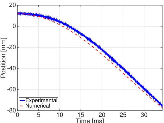
2.4 Comparison of the bench test data with the numerical ODE model

described in this section. . . 12

2.5 A photograph of the installed valve in a partially-opened position. . . 12

2.6 Left: Pitot pressure traces from a run with a diaphragm and a run with the valve. The effective opening time of the valve is about 40 ms

and the resulting run time is approximately 60 ms. Right: Power spectra of pitot pressure during the steady run time for a shot with

a diaphragm and a shot with the valve. The valve reduces the noise

level in the tunnel by a factor of about 2-3 across all frequencies.

High-frequency spikes in both spectra are due to electrical noise. . . 13

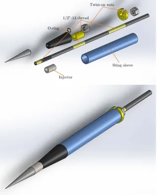
2.7 Both models used in this work. One has a cylindrical injector section

(top) and the other has a conical section (bottom). The ruler scale is in

inches. Republished with permission of AIAA. From Schmidt et al.

(2015); permission conveyed through Copyright Clearance Center,

Inc. . . 14

2.8 5x-magnified images of the surface of injectors. The red line in the

lower right corner of each image is 100 µm. Republished with

per-mission of AIAA. From Schmidt et al. (2015); perper-mission conveyed

(12)

2.9 Exploded view and assembly of solid model of the test article with

the cylindrical injector. Threaded segments of the aluminum tube are

colored yellow. Holes for the PCB pressure transducers are visible

on the frustum section. . . 16

2.10 Sketch illustrating 1-D porous flow. The porous media has thickness hand cross-sectional area A. If the flow is incompressible, the flow

rate is related to the pressure drop by Equation 2.1. . . 17

2.11 Sketch of porous flow through an axisymmetric geometry such as the

cylindrical injector used in this work. The injector has inner radius riand outer radiusro. . . 17

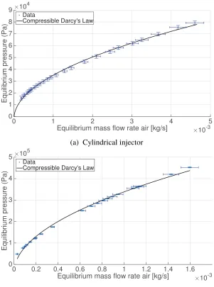
2.12 Pressure vs. mass flow rate data for air for both injectors fit with

Equation 2.13 to determine permeabilities. Republished with

per-mission of AIAA. From Schmidt et al. (2015); perper-mission conveyed

through Copyright Clearance Center, Inc. . . 20

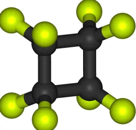
2.13 3-D model of an RC318 molecule. The black spheres represent

carbon atoms and the green spheres are fluorine atoms. Image by

Fvasconcellos - Own work, Public Domain. . . 21

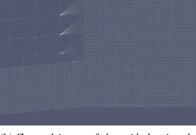
2.14 Refined computational grid for the OpenFOAM simulations. . . 26

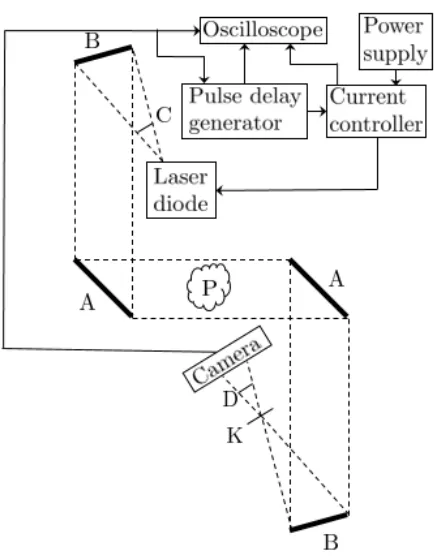
3.1 Schematic and wiring diagram for a schlieren imaging setup with a

pulsed laser diode light source. Light paths are shown as dashed

lines, electrical connections are solid arrows. A: turning mirror, B:

concave mirror (f = 150 cm), C: diverging lens, D: focusing lens, K:

schlieren cutoff, P: phase object. . . 31

3.2 Example timing diagram for the camera and light source. The timing

of this diagram is not specific to any particular experimental case but

is simply to show the desired scheme. Republished with permission

of AIAA. From Parziale, Damazo, et al. (2015); permission conveyed

through Copyright Clearance Center, Inc. . . 32

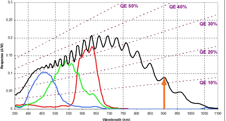
3.3 Spectral response chart for the Phantom v710 camera. The black

curve is the total response. The orange arrow marks 905 nm, the

wavelength of the laser light source. Chart ©Vision Research, Inc. . 33

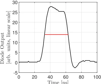
3.4 Output of the laser diode measured with a photodetector. The full

width at half maximum is shown in red, and is 30 ns for a nominal

(13)

4.1 Sketch of Fedorov’s hypothesis of a negatively-sloped injector

com-pensating for the additional displacement thickness created by

injec-tion. The graphic on the right shows the desired idealized shock

pattern on a cone model: only the shock at the tip of the cone is

present. Republished with permission of AIAA. From Schmidt et al.

(2015); permission conveyed through Copyright Clearance Center,

Inc. . . 36

4.2 Example schlieren images with the conical injector. The free stream

gas and injected gas for these cases is air. . . 37

4.3 Example schlieren images with the cylindrical injector. . . 38

4.4 Full-field images with a 40 ns-pulse width from three cases with

nitrogen injection at different injection rates. The injector is marked

by red lines and the PCB locations are shown with blue lines. . . 41

4.5 Full-field images with a 40 ns-pulse width from three cases with

different injected gases but the same value of δ. The injector is

marked by red lines and the PCB locations are shown with blue lines. 41

4.6 Injection layer thickness measured at the rear of the injector

sec-tion, normalized by the injection length, plotted versus the

non-dimensional mass flux F. High Reynolds number cases have a

nom-inal unit Reynolds number of 18×106per meter. . . 43

4.7 Transition location measured from the front of the injector section

plotted against the non-dimensional mass fluxF. . . 43

4.8 Images from a sample case to illustrate the image processing routine.

Images (a) through (e) represent stages in the routine with (a) being

the raw image and (e) being the final, processed image. . . 44

4.9 Processed image showing instability waves to be analyzed by

au-tocorrelation. The yellow dashed lines show the region used for

autocorrelation. . . 47

4.10 Autocorrelation curve for the image shown in Figure 4.9. The peak

at non-zero lag corresponds to a wavelength of 9 mm. . . 47

4.11 Histogram of measured wavelengths for an example case. The red

line shows a fitted log-normal distribution. . . 48

4.12 Wavelength normalized by the injector length plotted against the

non-dimensional injection rate F for all cases analyzed. The wavelength

is measured directly for helium and nitrogen injection and calculated

(14)

4.13 Series of images of a case with nitrogen injection showing the

prop-agation of waves. Their velocity is determined by cross correlating

the region in the images where the waves are present. . . 50

4.14 Correlation curve for the example case shown in Figure 4.13. The lag,

indicated by the red arrows, is converted to a velocity by multiplying

by the framing rate. . . 50

4.15 Distribution of measured velocities for the example case. . . 51

4.16 Convective velocity normalized by the free stream velocity plotted

versus the non-dimensional mass flux Ffor all cases studied. . . 51

4.17 Example image from a case with RC318 injection. The colored dots

on the left side of the image represent the location of the injection

layer edge determined by the Canny, log, Roberts, zero-cross, Prewitt,

and Sobel edge-detection methods. . . 52

4.18 Power spectral density plots from the Prewitt and Sobel methods for

the example RC318 injection case. Peaks are observed at 24.5 kHz

for both methods. . . 53

4.19 Response of the PCB pressure transducers in the cone frustum to

mechanical vibration. They are labeled in the figure legend according

to their distance from the cone tip, measured along the surface of the

model. . . 54

4.20 Spectra from the PCB pressure transducers for four example

experi-ments with injection. . . 55

4.21 Spectra from transducer 1 for the three injection cases shown in

Figure 4.20 compared to the turbulent baseline shown in Figure 4.20a. 56

4.22 Frequency from image analysis and pressure transducers. The

fre-quency from image analysis for the helium and nitrogen injection

cases is computed using Taylor’s hypothesis while the frequency in

the RC318 cases is computed directly from the image processing

routine. . . 57

4.23 Profiles taken at the rear of the injector section for the various grid

resolutions tested. . . 59

4.24 Relative difference in the flow variables plotted as a function ofyfor

the grid with a resolution of 69 µm/cell compared to the most refined

grid (38 µm/cell). . . 59

4.25 Total relative difference (see Equation 4.5) in flow variables as a

(15)

4.26 Results from the three computations with nitrogen injection.

Color-ing corresponds to density, with the color scale normalized to each

case. The value for the non-dimensional mass flux F is given in the

upper-left for each case. . . 61

4.27 Location of wall-normal profiles for all OpenFOAM cases. They

are located 120 mm, 132.5 mm, 152 mm, 172 mm, 180.6 mm,

189.2 mm, 197.8 mm, and 206.4 mm from the cone tip, measured

along the surface of the model. The case with nitrogen injection with u_inj =16 m/s is shown as an example. . . 61

4.28 Evolution of flow variables for cases with nitrogen injection. Profiles

are taken at the locations indicated in Figure 4.27. Black, blue, and

red curves correspond to cases with low, medium, and high rates of

injection listed in Table 4.1, respectively. . . 63

4.29 Mass fraction of injected nitrogen at the wall as a function of s, the

variable measured along the cone surface. Here, s = 0 corresponds

to the end of the injector section. Black, blue, and red curves

cor-respond to increasing injection rate with injection velocities listed in

the legend. . . 64

4.30 Results from the three computations with helium injection. Coloring

corresponds to density, with the color scale normalized to each case.

The value for the non-dimensional mass fluxFis given in the

upper-left for each case. . . 65

4.31 Evolution of flow variables for cases with helium injection. Profiles

4.32 Mass fraction of helium at the wall as a function of s, the variable

measured along the cone surface. Here, s = 0 corresponds to the

end of the injector section. Black, blue, and red curves correspond to

increasing injection rate with injection velocities listed in the legend. 68

4.33 Results from the three computations with RC318 injection. Coloring

corresponds to density, with the color scale normalized to each case.

The value for the non-dimensional mass fluxFis given in the

(16)

4.34 Evolution of flow variables for cases with RC318 injection. Profiles

4.35 Mass fraction of RC318 at the wall as a function of s, the variable

measured along the cone surface. Here, s = 0 corresponds to the

end of the injector section. Black, blue, and red curves correspond to

increasing injection rate with injection velocities listed in the legend. 72

4.36 Experimental measurements of the injection layer thickness measured

at the rear of the injector section compared with the displacement

thickness at the same location from the OpenFOAM computations

(indicated with "OF" in the legend). . . 73

4.37 Profiles taken at the rear of the injector section for cases with all three

injected gases. Cases are selected such that the value of δ?is similar

for all three. . . 76

4.38 Profiles taken 206.4 mm from the cone tip for cases with all three

injected gases. Cases are selected such that the value of δ?is similar

for all three. . . 77

5.1 δ, measured at the rear of the injector section, normalized by the

length of the injector Linjplotted against the dimensionless

momen-tum flux ratio J for all experimental and computational data. The

black line is a fitted power law curve considering only data from

nitrogen and helium injection cases. The expression for the curve is

given in Equation 5.3. The ⊕symbol indicates the tuned condition. . 79

5.2 Transition locationxtr, measured from the front of the injector section,

normalized by the injection layer thickness δmeasured at the rear of

the injector plotted against the velocity ratio of the injected gas to the

free stream gas. . . 81

5.3 Wavelength normalized by the injector length plotted against the

non-dimensional injection momentum flux J for all cases analyzed. The

wavelength is measured directly for helium and nitrogen injection

and calculated assuming Taylor’s hypothesis for RC318 injection.

(17)

5.4 Convective velocity normalized by the free stream velocity plotted

versus the non-dimensional momentum flux J for all cases studied.

Vertical error bars represent uncertainty due to measurement error,

including pixel-locking. . . 83

5.5 Frequency from image analysis and pressure transducers. The

fre-quency from image analysis for the helium and nitrogen injection

cases is computed using Taylor’s hypothesis while the frequency in

the RC318 cases is computed directly from the image processing

routine. . . 83

5.6 Sample image of instability waves in a cone boundary layer at a unit

Reynolds number of 9×106per meter. Yellow arrows indicate the

crests of three consecutive waves, and blue vertical lines indicate the

locations of the first four pressure transducers. The fifth transducer

is outside the viewing window of the camera to the right of the image

in the figure. . . 85

5.7 Spectra from the pressure transducers on a straight cone under the

same conditions as the visualization in Figure 5.6. The spectra show

growth of an instability around 46 kHz that breaks down to a

tur-bulence at or before the location of the final transducer. The insert

shows the spectrum of the first transducer so that the peak at 45.9 kHz

can be clearly perceived. . . 86

5.8 Sketch of a two-dimensional free shear layer flow. Two streams with

different velocities and potentially different densities and specific

heats are initially separated by a splitter plate and allowed to mix

downstream of the plate. A mean velocity profile is sketched in the

mixing region. Stream 1 is the high-speed stream and stream 2 is the

low-speed stream by definition. . . 88

5.9 Streamlines in a frame convecting with structures in a shear layer.

There are stagnation points for each stream between the structures. . 91

5.10 Example momentum profile for a case with nitrogen injection. The

curvature thickness δcis indicated with black dashed lines. . . 92

5.11 Wavelength normalized byδcusing the values in Table 5.1 for the

ex-periments performed with the lower unit Reynolds number condition

(18)

5.12 Ratio of the measured experimental value of wave convective speed

to that predicted using Equation 5.14 (tabulated in Table 5.2) plotted

againstJfor cases with a nominal unit Reynolds number of 9×106per

meter. . . 95

5.13 Convective Mach numberMcplotted as a function of the wall-normal

coordinateyfor three example cases. Profiles are taken at the rear of

the injector section. . . 97

A.1 Schmidt number as a function of temperature for each injected gas

diffusing into nitrogen. . . 118

A.2 Comparison of results of the diffusion box test case for nitrogen. . . 119

A.3 Comparison of results of the diffusion box test case for nitrogen

assumingSc= 1 in Equation A.8. . . 120

A.4 Comparison of results of the diffusion box test case for helium. . . . 120

A.5 Comparison of results of the diffusion box test case for RC318. . . . 121

C.1 Schematic of an FLDI setup. The two beams are shown as blue and

green. Regions where the beams overlap are shown as striped. The

coordinate system shown will be the one used throughout this paper. 145

C.2 Illustration of a prism (here, a Wollaston prism). The incident beam

of aribtrary polarization is split into two beams by an angle σ, and

the two beams at the exit have mutually orthogonal polarization. The

ordinary ray is linearly polarized in the direction of beam separation

and the extraordinary ray is polarized 90 degrees from the direction

of separation. . . 145

C.3 Computed beam widths (out to 1/e2) within 30 mm of the best focus.

One beam is outlined in red and the other in blue. The width of the

beams at the waist is too small to see on this scale. . . 150

C.4 Polar grid cross-section non-dimensionalized by the local beam waist

size . . . 151

C.5 Transfer functionHw(k)for a single beam for 1-D sinusoidal distur-bances in xin an infinitesimally-thin plane at z =0 . . . 154

C.6 Transfer function of Equation C.16 plotted for various values ofL. As Lincreases, or, as more signal away from best focus is considered, the

error function in Equation C.16 contributes a k−1 rolloff beginning

at lower values of k. This leads to attenuation of high-wavenumber

(19)

C.7 Transfer functionHw(k)for a single beam for uniform 2-D sinusoidal disturbances in xbetween z= ±10 mm centered atz =0. . . 155

C.8 Transfer functionHw(k)for a single beam for uniform 2-D sinusoidal disturbances in xbetween z= ±30 mm centered atz =0. . . 156

C.9 Transfer function H(k) for the two-beam FLDI for 1-D sinusoidal

disturbances in xin an infinitesimally-thin plane at z= 0. . . 157

C.10 Transfer function H(k) for the two-beam FLDI for uniform 2-D

sinusoidal disturbances in xbetween z= ±10 mm centered atz =0. 158

C.11 Transfer function H(k) for the two-beam FLDI for uniform 2-D

sinusoidal disturbances in xbetween z= ±30 mm centered atz =0. 158

C.12 Convergence study for the transfer function shown in Figure C.11.

The red square indicates the chosen resolution. . . 159

C.13 Normalized FLDI output signal for sinusoidal disturbances within

±_{10 mm of the focus in} z, corresponding to the transfer function

plotted in Figure C.10. . . 160

C.14 A solid model of the chamber for the argon jet with dimensions given

in mm. The coordinate system shown corresponds to the orientation

of the coordinate system of the FLDI beams. . . 161

C.15 . . . 161

C.16 Steady-state result of OpenFOAM computation of the flow out of the

argon jet. Velocity vectors are shown on the left and streamlines on

the right. Both are superimposed on a contour plot of argon mass

fraction. Ljetis the length out of the page (inz) that the cross-section

shown here extends. . . 162

C.17 Index of refraction field from the OpenFOAM computation with

spline interpolation. . . 163

C.18 Experimental vs. numerical data for the argon jet experiments

de-tailed in Table C.2. The letters marking each data point correspond

to the configurations in Table C.2. The line is the ideal liney = x. . . 164

C.19 Cone model used in T5 studies . . . 167

C.20 . . . 168

C.21 Output of the FLDI simulation compared to the input boundary layer

wave packet density disturbance. The y-axis on the left corresponds

to the FLDI output and the y-axis on the right corresponds to the

(20)

C.22 Output of the FLDI simulation, scaled with Equation C.27, compared

to the input boundary layer wave packet for the optimum value of Z =12.6 mm. . . 171

C.23 PSD of the FLDI simulation, scaled with Equation C.27 and optimum

Z value, compared to the PSD of the input boundary layer wave

packet. . . 171

(21)

LIST OF TABLES

Number Page

2.1 Properties of injected gases at 295 K. . . 21

2.2 Sutherland coefficients for the three injected gases to be used in calculating viscosity in Equation 2.18. . . 23

4.1 Flow conditions for the OpenFOAM computations. . . 58

4.2 Estimated Gladstone-Dale constants for the three gases at a wave-length of approximately 600 nm and room temperature with the com-puted displacement thicknesses and thicknesses based on index of refraction calculated at the rear of the injector section for cases with u_inj = 16, 40, and 3 m/s for nitrogen, helium, and RC318 injection, respectively. . . 75

5.1 Values of δc for momentum profiles at the beginning of the injector section for the OpenFOAM computations. . . 93

5.2 Values of UU∞c computed with Equation 5.14 and the data from the OpenFOAM computations using the lower point of curvature in the momentum profile to determine the conditions in stream 2. Profiles are taken at the rear of the injector section. . . 95

A.1 Parameters from the Lennard-Jones potential model for the three gases for computing diffusion coefficients. . . 117

C.1 Optical parameters for simulated FLDI. . . 148

C.2 Argon jet configurations tested (dimensions in mm). . . 163

C.3 Boundary layer edge conditions for T5 shot 2789. . . 166

C.4 Boundary layer wave packet parameters. . . 169

(22)

C h a p t e r 1

INTRODUCTION

Injection of gas into boundary layers in hypersonic flight has the potential to enable

the next generation of high speed vehicles. Flight at hypersonic Mach numbers

presents a unique set of challenges, among which are high heating loads that create a

need for thermal protection systems and challenges related to supersonic combustion

ramjet (scramjet) propulsion. Figure 1.1 shows a sketch of a typical injection system

and flow field. In this example, gas is injected orthogonally to the mean flow direction

through a porous section in the wall. Injection modifies the velocity profile in the

boundary layer as shown in the figure, and also changes the temperature, density, and

sound speed profiles. Injection also creates a sudden increase in the displacement

thickness of the boundary layer which causes a shock to form in the supersonic free

stream. In this work the boundary layer downstream of injection is referred to as the injection layerto avoid confusion with conventional boundary layers.

Figure 1.1: Sketch of the flow field associated with injection into a supersonic flow. Velocity profiles are shown in blue before and after injection.

The problem of injection into high speed boundary layers has been studied

inter-mittently over the last half-century for a variety of reasons. The following section

reviews some of this research. The work presented here addresses some of the

remaining challenges associated with transition to turbulence in these flows.

1.1 Applications of Injection

This section outlines four of the applications for injection into high-speed boundary

(23)

cooling, a surrogate for studying ablation, transition delay in hypervelocity boundary

layers, and enhancement of scramjet performance. For a more complete discussion

of the past work on this topic related to the first two applications, see Schneider

(2010).

Film and transpiration cooling

Heating in high speed boundary layers is a significant issue that creates a need for

substantial thermal protection systems on hypersonic vehicles. Traditionally these

systems are passive, such as the ceramic tiles on the Space Shuttle. The primary

drawback of such a system is additional vehicle weight, although lack of reusability

due to ablation of the protective material is also a concern. Gas injection has been

considered as an active thermal protection system because the layer of cold gas next

to the vehicle surface behind the injector has a cooling effect (Aupoix et al., 1998;

Cary and Hefner, 1971; Sahoo et al., 2005). The cold injected gas displaces the hot

boundary layer fluid away from the vehicle surface, leading to a reduction in heat

transfer. See e.g. Figure 7 of Marvin and Akin (1970). When the injected gas is

blown tangentially to the surface of the vehicle it is referred to as film cooling, and

orthogonally injected gas through a porous surface is called transpiration. Both of

these have been studied in the literature.

Transpiration and film cooling are more effective in high speed flows than low

speed flows, but covering the entirety or even the majority of a vehicle with such

a thermal protection system is likely impractical and the weight savings compared

to traditional passive systems may not be significant. Localized cooling, however,

remains promising. Local cooling would allow placement of a window or instrument

on the surface of a vehicle, which would not be possible if a passive system were

used. An injector placed directly upstream of the instrument could cool that area

actively while the rest of the vehicle is covered by a traditional passive system.

Egorov et al. (2015) performed a numerical study on a blunt geometry and showed

that such a scheme could be effective. Cooling in this type of an arrangement

is most effective while the interface between the injected gas and the free stream

fluid remains laminar. Turbulence enhances mixing of the streams and therefore

decreases cooling. This can be observed in Figure 7 of Marvin and Akin (1970)

where the heating rate returns to its value prior to gas injection after transition to

(24)

Ablation surrogate

Ablation is an extremely complex phenomenon as it involves the coupling of a host

of effects including non-equilibrium gas dynamics, chemical reactions, outgassing,

boundary layer stability, turbulence, and heat transfer. Understandably, then,

re-searchers have sought to isolate some of the effects and study each in turn. Gas

injection has been studied for this reason to decouple the outgassing of pyrolysis

products from the other features of flow with ablation.

Some studies have concentrated on blunt geometries such as reentry capsules (Li

et al., 2013), while others have instead focused on slender bodies (Marvin and

Akin, 1970; Pappas and Okuno, 1960, 1964). The works cited here represent

investigations where the stability and transition of the flow were considered. Pappas

and Okuno (1960) observed that transition occurs earlier on a porous cone when

higher blowing rates are employed and when the molecular weight of the injected gas

is lower. This trend is corroborated in many other studies as well (Schneider, 2010),

but Li et al. (2013) curiously found computationally that transpiration stabilized the

second-mode instability on a flat plate and cone. The results of the current study

could be extended to ablation like the investigations cited in this section, but this is

not pursued here.

Transition delay

Boundary layer transition in hypersonic flows is dominated by thesecondor Mack mode, particularly when the wall is cold compared to the adiabatic wall temperature

as is the case in hypersonic free flight (Mack, 1984). Current understanding of the

Mack mode is summarized by Fedorov (2011) and Fedorov and Tumin (2011) and

the interested reader is referred to these for further information. Fujii and Hornung

(2001) and Wagnild et al. (2009) have shown that the strength of the Mack mode

instability can be reduced via acoustic absorption by non-equilibrium effects in

the boundary layer gas. This occurs if the time scale of translational/rotational and

vibrational energy exchange in the gas molecules is on the same order as the acoustic

waves responsible for destabilizing the boundary layer (typically about 1 MHz) and

if the vibrational energy states in the gas are sufficiently populated. Both of these

conditions are met for carbon dioxide in hypersonic flows.

Leyva et al. (2009) and Jewell et al. (2012) performed experiments in the T5

hy-pervelocity shock tunnel at Caltech to determine if transpiration of carbon dioxide

(25)

transition. The injector in these studies was approximately 40 mm long and began

135 mm from the cone tip.

The data from these studies suggest a delay in transition for carbon dioxide injection

compared to argon injection, which would not have the non-equilibrium effects

required for acoustic absorption. They are inconclusive, however, regarding the

overall efficacy of carbon dioxide injection versus no injection. The results are

further complicated by the fact that Fedorov, Malmuth, et al. (2001) showed that

a porous surface such as the one on the injector section absorbs acoustic energy

and therefore contributes to stabilization of the Mack mode. Furthermore, Fedorov,

Soudakov, et al. (2014) found that injection in such a configuration has a destabilizing

effect when non-equilibrium effects are not considered. More work is warranted

on this subject, but the current study focuses on low-enthalpy flow where

non-equilibrium effects are not important and therefore the potential application of

transition delay in hypersonic boundary layers is not kept in mind.

Scramjet performance

Scramjet engines are considered by many to be the best method for propulsion at

very high Mach numbers in the atmosphere, and improving scramjet performance is

an active research topic. Gas injection in scramjet inlets in particular has a number

of promising benefits. In this application a small fraction of the vehicle’s fuel is

injected in the inlet prior to the gas reaching the combustor, where the remainder of

the fuel is injected.

Barth, Wheatley, et al. (2013) demonstrated that injection in scramjet inlets not only

produces the cooling effect described earlier in this section, but also significantly

reduces skin friction drag. This is important because skin friction drag in the inlet

forms a substantial fraction of the total scramjet drag, as much as 25%. The effect

is enhanced if combustion occurs. The mechanism seems to be twofold. First, the

modification of the velocity profile reduces the slope of the velocity curve at the

wall, thereby reducing skin friction. Secondly, combustion causes dilatation that

further favorably modifies the velocity profile and the temperature rise associated

with combustion reduces the magnitude of turbulent velocity fluctuations, which in

turn reduces the Reynolds shear stress.

Second, flow separation due to compression in scramjet inlets is a potential issue

that can degrade performance. Laminar boundary layers are more prone to

(26)

employed to encourage transition to turbulence (Berry et al., 2001). Injection

desta-bilizes the boundary layer, so injection in the engine inlet could eliminate the need

for physical trips.

Finally, Gehre et al. (2015) and Barth, Wise, et al. (2015) show that if the injected

fuel in the inlet mixes sufficiently with the air in the free stream and is combusted,

significant gains are made in overall engine efficiency. These gains are primarily

due to the production of radical species and heating in the inlet region that promote

combustion in the combustor. All of these effects are much stronger if the interface

between the injected gas and the free stream is turbulent.

1.2 Remaining Issues

The current study is focused on addressing issues related to the implementation of

injection for localized transpiration cooling and fuel injection in scramjet inlets.

Attention is given to the mechanics of the flow field and although the results of this

work have design implications, the design of an injection system is not considered

directly. Effects are subdivided into inviscid and viscous categories.

Formation of waves

Transpiration causes an abrupt increase in the displacement thickness of the

bound-ary layer, which the free stream perceives the same as a change in the geometry of the

body. The supersonic flow is turned in response to these changes by oblique shock

waves and expansion waves. The strength of the shock waves is dependent on the

injection rate and body geometry, but they can be strong enough to be detrimental

to performance, particularly in internal flows.

For instance Ogawa et al. (2015) found that the shock wave formed at the beginning of

the injector in a scramjet inlet was reflected several times in the narrow channel and

caused substantial pressure losses depending on the injection rate. They found that

for their geometry the benefits of injection were counteracted by the total pressure

loss. The amount of fuel that could be injected while maintaining a net benefit was

also limited to avoid larger pressure losses.

Wave formation is more important in internal flows than external flows, but Schmidt

et al. (2015) demonstrate that the shock wave at the beginning of the injector in an

external flow can be strong enough to create an adverse pressure jump capable of

causing the incoming boundary layer to transition to turbulence. Effective cooling

(27)

to turbulence would substantially limit the usefulness of transpiration for cooling.

The mitigation of waves is therefore important for the implementation of injection

systems for both applications considered.

Flow stability

Clearly in both applications the state of the boundary layer downstream of injection,

whether laminar or turbulent, is of importance. A laminar injection layer is crucial

for effective cooling because of reduced transport of heat compared to a turbulent

layer. In scramjet inlets, turbulence decreases the efficacy of cooling at the wall, but

it also substantially promotes mixing which is necessary for efficient combustion.

Combustion must occur in the inlet in order for the benefits of injection to be fully

realized.

Even so, the stability of this flow has not been studied in great detail. The vast

majority of experimental data pertaining to stability are transition locations, and

though these are useful, they contribute little to the understanding of the underlying

physics of the transition process. A handful of numerical studies have been

per-formed to analyze stability characteristics of supersonic flows with injection, e.g. Li

et al. (2013), but experimental measurements are scarce (Schneider, 2010). Flow

stability with injection of a foreign gas, i.e. one that is different from the free stream

gas, is more difficult to analyze computationally because fluid properties are

depen-dent on the local composition, which means that the transport equations are coupled

to the Navier-Stokes equations. Stability studies of this kind are even more rare,

but in most practical applications of injection the injected gas would differ from

the free stream gas. These factors motivate an experimental investigation of the

stability properties of supersonic flow with injection, including injection of foreign

gas species.

1.3 Project Scope and Outline

The instability in supersonic flow with injection is analyzed in this work. A method

for diminishing the strength of waves formed by injection by modifying the body

geometry is also presented. Experiments are performed in the Caltech Mach 4

Ludwieg tube with a 5-degree half-angle cone as the base model because of its

canonical shape. Injection is achieved by transpiration through a porous injector

section on the model, and three gases with different molecular weights are injected.

The primary aim of the study is to characterize the disturbances that lead to transition

(28)

The Ludwieg tube facility and the test article are described in Chapter 2 along with

computations of the base flow. The choice of injected gases is also explained. In

Chapter 3 the high-speed schlieren technique used to measure instability waves in

the flow is described and is accompanied by a review of potential measurement

techniques that were also considered. Results of the experiments are given in

Chapter 4. Data processing routines are also presented in this chapter. The results

(29)

C h a p t e r 2

FACILITY & TEST PROCEDURE

The test facility and experimental apparatus are presented in this chapter. The

Ludwieg tube is described with special attention given to modifications made to the

facility for the current work. The test article is then described and the flow through

the porous injector section is analyzed. The choice of injected gases is explained

and the properties of the gases are given. The flow meter and calibration technique

are also described. Finally, the setup for numerical simulations of the experiments

in OpenFOAM is presented.

2.1 Ludwieg Tube

Experiments for this work were performed in the Caltech Ludwieg Tube. The facility

is described in detail by Mouton (2007) and summarized here. It consists of a 17

m-long, 300 mm-diameter tube, a nozzle, test section, and dump tank. Experiments in

this work exclusively use the axisymmetric Mach 4 nozzle described in Section 6.2

of Mouton (2007). The nozzle has an exit diameter of 315 mm. A perspective view

of the Ludwieg tube is shown in Figure 2.1.

Figure 2.1: Solid model of the Caltech Ludwieg tube shown with the Mach 4 nozzle. The overall length of the facility is 23.5 m. Republished with permission of AIAA. From Schmidt et al. (2015); permission conveyed through Copyright Clearance Center, Inc.

Most Ludwieg tubes use diaphragms to separate the high- and low-pressure sections.

(30)

to here as a downstream diaphragm configuration, or just ahead of the nozzle

contraction, called an upstream diaphragm configuration. When it is operated with a

diaphragm, the Caltech Ludwieg Tube uses an upstream diaphragm configuration as

shown in Figure 2.2 because the facility has issues with starting when a downstream

diaphragm is used. This is described in Section 6.3 of Mouton (2007). When

operated with a diaphragm, the nozzle, test section, and dump tank are evacuated

and the driver tube is pressurized until the diaphragm ruptures. When the diaphragm

breaks, a weak shock wave propagates through the nozzle and test section and a

non-steady expansion wave propagates away from the nozzle in the driver tube and

reflects from the tube end wall. These processes establish steady supersonic flow

in the test section, and the reservoir conditions upstream of the nozzle contraction

remain constant until the reflected expansion wave returns to the nozzle-driver tube

junction.

Tube

Diaphragm location

Nozzle _SectionTest

Figure 2.2: Section view of the Ludwieg tube nozzle with the upstream diaphragm station labeled. Flow is from left to right.

Nitrogen is used as the test gas in this work, and the reservoir temperature in the

driver tube is nominally 297 K. The driver pressure can be varied between 100 and

600 kPa, but is determined by the strength of the diaphragm used when the facility

is operated with a diaphragm. Assuming quasi-1D, isentropic flow of a perfect gas

with a free stream Mach number of 4.0, the free stream temperature is 68 K, the

velocity is 672 m/s, and the unit Reynolds number is between 5−25×106per meter

depending on the reservoir pressure. The maximum test time is fixed by the length

of the driver tube and is approximately 100 ms.

2.2 Pneumatic Valve

Operating the facility with a diaphragm has several drawbacks. First, the stagnation

pressures that can be accessed are limited by commercially available diaphragms.

Polycarbonate film diaphragms are used, and can only be bought in thicknesses of

(31)

used. The strength of a diaphragm with a given thickness varies, however, making

it difficult to repeat test conditions precisely. Second, the broken diaphragm creates

disturbances that propagate into the test section, adding to the free stream noise level

of the facility. Finally, the diaphragm needs to be changed after each run, placing a

lower limit on the turnaround time of about 30 minutes.

To address these issues, a fast-acting valve based loosely on the one used in the

Hypersonic Ludwieg tube Braunschweig (HLB) (Estorf et al., 2003) was designed

and installed in the Caltech Ludwieg Tube to replace the diaphragm. A solid model

of the installed valve is shown in Figure 2.3. The primary component of the valve is

a pneumatic cylinder that is suspended in the center of the Ludwieg tube driver. A

plug is attached to the shaft of the cylinder, which creates a seal in the nozzle throat,

separating the high pressure driver from the low-pressure test section until the run

begins, just as a diaphragm would. Operation is as follows. The upstream side of

the cylinder is pressurized with the downstream side open to the ambient air in the

laboratory, moving the plug into the throat of the nozzle (top of Figure 2.3). With

the plug in place, the nozzle, test section, and dump tank are evacuated while the

driver tube is pressurized with the test gas. When the desired stagnation pressure

is reached in the driver section, the upstream side of the cylinder is opened to

the laboratory air and the downstream side is pressurized. When the force on the

piston inside the cylinder becomes sufficiently high to overcome the force due to

the pressure difference across the plug, the plug quickly moves out of the nozzle

throat and joins with the cylinder housing, forming a smooth center body (bottom

of Figure 2.3). Steady flow in the test section is achieved once the plug is secure

against the housing.

Besides the requirement that the valve fit inside a 16.2 cm-diameter shroud, the

primary requirement for the valve is that the plug must move far enough to fully

retract from the converging part of the nozzle while leaving sufficient time for

steady test flow once the valve is open, and it must not recoil upon reaching the

open position. The design point is 15 cm in 20 ms for a 500 kPa stagnation pressure

condition. Opening time is expected to be longer than this for lower-pressure

conditions, but as long as the opening time is sufficiently less than 100 ms the tunnel

will still have a satisfactory steady run time. Operation of the pneumatic cylinder

is modeled assuming isentropic expansion and compression inside the cylinder and

quasi-steady Fanno flow through the exhaust line which is open to the atmosphere

(32)

upstream section

(a)

(b)

downstream section

1.04m

Figure 2.3: Section view of the Ludwieg tube with the valve installed. The valve is shown in both the closed (a) and open (b) positions. The sections of the cylinder are labeled upstream and downstream corresponding to the direction of flow in the Ludwieg tube.

once the piston begins to move. These assumptions lead to a system of three

ODEs describing a nonlinear spring-mass-damper system and can be integrated

numerically using standard Runge-Kutta methods.

The valve was bench tested to validate the numerical model using string to hold the

plug in place to simulate the pressure difference during a run. The string was cut

to simulate the start of a run after pressurizing the cylinder. The position of the

plug was measured with a Keyence LK-G407 laser range finder. Figure 2.4 shows a

comparison between the numerical ODE model and the performance of the valve,

indicating the utility of the model for design purposes.

The valve was designed iteratively with the numerical solution to the model until a

suitable design was obtained. To minimize cost, the cylinder chosen is an

off-the-shelf Parker pneumatic cylinder. The piston is enclosed in a streamlined cylindrical

shroud to minimize perturbation to the flow. The sealing face of the plug, shown in

black in Figure 2.3, is made from polyurethane and is designed to match the slope

of the nozzle contour when the piston is in the closed position. The end of the plug

is made from aluminum and is a streamlined shape. The cylindrical shroud is made

from PMMA and the upstream end of the shroud is rapid-prototyped nylon to reduce

the weight of the structure. Its shape is an ellipsoid and the surface is roughened to

encourage boundary layer transition and therefore minimize flow separation at the

(33)

Time [ms]

0 5 10 15 20 25 30

Postition [mm]

-80 -60 -40 -20 0 20

Experimental Numerical

Figure 2.4: Comparison of the bench test data with the numerical ODE model described in this section.

compressed gas cylinders used to fill the driver tube. A photograph of the installed

valve is shown in Figure 2.5.

Figure 2.5: A photograph of the installed valve in a partially-opened position.

Figure 2.6 shows the free stream pitot pressure traces and spectra for nominal

300 kPa-reservoir pressure runs with a diaphragm and the valve. The left-hand plot

shows that the opening process of the valve reduces the total test time from 100 ms

to about 60 ms. This is not detrimental, however, as 60 ms still provides for over

(34)

valve reduces the noise in the stagnation pressure across all frequencies by a factor

of 2-3. The RMS noise level in stagnation pressure is reduced from 1-2% to 0.7%.

103 104 105

10−6

10−4

10−2

Frequency [Hz]

(

p

′/0

¯

p0

)

2

Diaphragm Piston

Figure 2.6: Left: Pitot pressure traces from a run with a diaphragm and a run with the valve. The effective opening time of the valve is about 40 ms and the resulting run time is approximately 60 ms. Right: Power spectra of pitot pressure during the steady run time for a shot with a diaphragm and a shot with the valve. The valve reduces the noise level in the tunnel by a factor of about 2-3 across all frequencies. High-frequency spikes in both spectra are due to electrical noise.

The other advantages of the valve over operation with the diaphragm are that the

tunnel can be operated at any pressure between the limits of 100 kPa and 600 kPa

instead of only those determined by available diaphragms. Test conditions are also

now repeatable to within a few percent (see e.g. Appendix D). Additionally, the

Ludwieg tube does not need to be opened after each run to replace a diaphragm, so

the turnaround time is reduced from 30 minutes to about 12 minutes. The remaining

gas in the driver tube after a run does not need to be evacuated after each experiment

as it does when using a diaphragm, so there is also a cost savings associated with

using less gas in the driver per shot along with the cost savings of no longer needing

to purchase diaphragms to operate the tunnel.

2.3 Test Articles

Two test articles are used in this work, both based on a sharp-tipped 5 degree

half-angle cone. The tip radius is measured to be 300 µm. This radius is sufficiently

small that the entropy layer is swallowed before the injector section is reached and

therefore the cone tip can be treated as sharp (Stetson, 1987). The models are shown

in Figure 2.7. Both have an aluminum tip section that is 131 mm long measured

along the surface of the cone, followed by a 40 mm long injector section, followed by

a frustum. The frustum is made from Delrin, a machinable plastic. One model has a

(35)

other has a cylindrical injector, and this article is used to analyze the instability in

the flow. The frustum section of this model is instrumented with five PCB 132A31

piezoelectric pressure transducers along its length.

Figure 2.7: Both models used in this work. One has a cylindrical injector section (top) and the other has a conical section (bottom). The ruler scale is in inches. Republished with permission of AIAA. From Schmidt et al. (2015); permission conveyed through Copyright Clearance Center, Inc.

The injectors are manufactured by Mott Corporation and are made of sintered

stainless steel. The surface area of the injectors is 2.66 ×10−3 m2. Magnified

images of the injectors are shown in Figure 2.8.

(a) Conical injector (b) Cylindrical injector

Figure 2.8: 5x-magnified images of the surface of injectors. The red line in the lower right corner of each image is 100µm. Republished with permission of AIAA. From Schmidt et al. (2015); permission conveyed through Copyright Clearance Center, Inc.

The models are assembled on a 1/2-inch diameter aluminum tube. The cone tip,

injector, and rear frustum interlock. The cone tip has 1/2”-13 internal threads to

(36)

injector to facilitate the flow of gas from the tube to the injector. An O-ring at the

rear of the frustum section ensures that gas does not escape through the rear of the

model. Sections of the tube are threaded and twist-on 1/2”-13 nuts are used on these

sections. One nut tightens the frustum, injector, and cone tip together. The other

tightens against the sting sleeve, which interlocks with the back of the frustum. The

sting sleeve fits in the sting in the Ludwieg tube test section. A plastic end cap is

used between the back of the sting sleeve and the corresponding twist-on nut, and

a slot is cut in the end cap to allow wires from the PCB sensors to pass through.

A 1/2-inch Swagelok fitting is fixed to the rear end of the aluminum tube which

mates with the injected gas plumbing line. A solid model of the assembly and an

exploded view are shown in Figure 2.9. Machine drawings for the parts, including

the pneumatic valve components, are included in Appendix B.

Porous Flow Analysis

The flow through the porous material of the injectors is modeled using the

compress-ible version of Darcy’s Law. Darcy’s Law is a well-known relation between the flow

rate and pressure difference for low Reynolds number flows through porous media

(Dullien, 1979). The derivation is straightforward from conservation of momentum.

The 1-D, steady, incompressible equation is

Q= κA µ

p₁− p₂

h , (2.1)

whereQis the volumetric flow rate,p1andp2are the pressures at the beginning and

end of the porous media section, respectively,his the thickness of the media,Ais the

cross-sectional area, µis the viscosity of the fluid, and κ is the permeability of the

media (see Figure 2.10). Permeability is the key parameter that relates the pressure

drop to the flow rate and has units of area. It must be determined experimentally.

A compressible version of Equation 2.1 can be derived from the continuity and

momentum equations. The analysis here follows closely that of Shepherd and

Begeal (1988). The injectors in this work are axisymmetric, so the continuity

equation is

d

dr ρu

+ ρu

r =0 , (2.2)

which reduces to

ρur = m˙

2πL = constant (2.3)

for a cylinder of lengthL, where ˙mis the mass flow rate. The geometry is shown in

(37)

Figure 2.9: Exploded view and assembly of solid model of the test article with the cylindrical injector. Threaded segments of the aluminum tube are colored yellow. Holes for the PCB pressure transducers are visible on the frustum section.

The momentum equation is a balance between viscous forces and the pressure drop

across the porous material:

−dp

dr =

ρu2_C_D

¯

d . (2.4)

In this expression ¯d is a characteristic length of the porous material. A common

assumption is that the media can be approximated as a bed of closely-packed spheres.

In this case ¯dis the mean sphere diameter.

CD is a drag coefficient for the media. If the Reynolds number based on ¯d (Red¯) is

(38)

Figure 2.10: Sketch illustrating 1-D porous flow. The porous media has thicknessh and cross-sectional area A. If the flow is incompressible, the flow rate is related to the pressure drop by Equation 2.1.

Figure 2.11: Sketch of porous flow through an axisymmetric geometry such as the cylindrical injector used in this work. The injector has inner radius ri and outer radiusro.

the drag coefficient:

CD =

¯ d2

κ 1 Re_d_¯ +

λ ¯ d

!

. (2.5)

κis again the permeability of the media, andλis the Forchheimer constant, which is a

property of the media that must also be determined experimentally. The Forchheimer

constant can be related to the permeability by the Carman-Kozeny expression for

the permeability of a bed of packed spheres:

κ = d¯23

180(1−)2

(39)

and the Ergun relation for the Forchheimer constant:

κ λ =

¯ d3

1.8(1−) . (2.7)

in these equations is the porosity, or volume fraction of empty space, of the porous

material (Macdonald et al., 1979). According to the manufacturer of the injectors

this is equal to 0.4. Equations 2.5, 2.6, and 2.7 can be combined to give

CD =

¯ d κ µ ρu + ¯ d

100(1−)

!

. (2.8)

A set of experiments was performed to simultaneously measure the pressure inside

the injectors and the gas mass flow rate using a Kulite XT-190 piezoresistive pressure

transducer and a Sensirion EM1 flow meter, respectively, to determine the properties

of the porous media. The two terms in Equation 2.8 can first be compared to

determine if both are necessary to model the flow through the injectors. According

to the manufacturer, the mean pore size is on the order of 10µm, so this can be used

as an estimate for ¯d that is assumed to be accurate within an order of magnitude.

The viscosity of air at room temperature is 1.9×10−5kg/m s, and the largest mass

flow rate in this set of calibration experiments is 4.5 g/s. Using these values, the

second term in Equation 2.8 is at most 5% of the first term and can be neglected.

This simplifies the expression for the drag coefficient to

CD =

¯ dµ

κ ρu . (2.9)

Equation 2.9 can be substituted into Equation 2.4 to give

−dp

dr = uµ

κ . (2.10)

The velocityucan be expressed in terms of the mass flow rate by using Equation 2.3:

−ρdp

dr = ˙ mµ

2πLκr . (2.11)

Equation 2.11 is integrated frompito poin pand from Ri toRoinr by expressing

the density as a function of pressure using the ideal gas law and assuming isothermal

flow through the porous media. The resulting expression is

p2

i −p2o=

˙ mµRT

πLκ ln ro

ri

!

(40)

In the experiments performed in this work the pressure outside the injector is of the

order 1 kPa while the pressure required to drive flow through the injector is of the

order 100 kPa, so p2o << pi2 and p2o can be neglected in Equation 2.12. The final

relation between pressure and mass flow rate is

p2

i =

˙ mµRT

πLκ ln ro

ri

!

. (2.13)

From Equation 2.13, it is clear that if pressure and mass flow rate are measured

simultaneously then the permeability κ is the only unknown parameter and can be

determined by linear least squares. Figure 2.12 shows the data from the calibration

experiments with a fit of Equation 2.13 to determine the permeability. κis equal to

3.5±.003×10−12m2for the cylindrical injector and 1.1±.0006×10−14m2for the

conical injector. Uncertainties are determined by the 95% confidence interval of the

least-squares fit and the measurement uncertainties in pressure and mass flow rate.

These values are typical of those reported for sintered stainless steel (Frederking

et al., 1986).

2.4 Injected Gases

Pappas and Okuno (1960) observed that the molecular weight of the injected gas

affects the transition location on a porous cone in Mach 4.8 flow. The choice of

injected gas is therefore considered to be an important parameter in the investigation

of the instability that leads to transition in this work. Nitrogen was chosen as one

injected gas because it is simpler to model since the free stream gas is also nitrogen

and diffusion of species need not be considered. Helium was selected as a second

injected gas because it is the lightest gas available (that does not require additional

safety measures to use) and therefore produces the largest deviations in behavior. The

properties of helium are similar to those of hydrogen which is a candidate scramjet

fuel, making it particularly relevant to the application of injection in scramjet inlets.

Helium is approximately seven times lighter than nitrogen, so a gas that is seven

times heavier than nitrogen (a molecular weight of 196 g/mol) was sought as the

final injected gas. Most substances with molecules of that size are not gases at room

temperatures, and many that are gases are highly toxic, corrosive, combustible,

and/or prohibitively expensive. Refrigerants were seen as a category of fluids that

may fit the criteria of being a gas at room temperature, non-toxic, compatible with

most materials, non-reactive, and reasonably priced. One refrigerant, RC318, fits

(41)

Equilibrium mass flow rate air [kg/s] _×10-3

0 1 2 3 4 5

Equilibrium pressure (Pa)

×104

0 1 2 3 4 5 6 7 8 9

Data

Compressible Darcy's Law

(a) Cylindrical injector

Equilibrium mass flow rate air [kg/s] _×₁₀-3

0 0.2 0.4 0.6 0.8 1 1.2 1.4 1.6

Equilibrium pressure (Pa)

×105

0 1 2 3 4 5

Data

Compressible Darcy's Law

(b) Conical injector

Figure 2.12: Pressure vs. mass flow rate data for air for both injectors fit with Equation 2.13 to determine permeabilities. Republished with permission of AIAA. From Schmidt et al. (2015); permission conveyed through Copyright Clearance Center, Inc.

ball-and-stick model of an RC318 molecule. The black spheres represent carbon

atoms and the green spheres are fluorine atoms.

RC318 is a fluorocarbon, its IUPAC name is octofluorocyclobutane. It is effectively

a cyclobutane molecule where all the hydrogen atoms have been replaced with

fluorine atoms. It has few documented applications, but is used in the production

of semiconductor materials and is therefore readily available. It is chemically inert

under most conditions, as the carbon-fluorine bond is extremely strong, often listed

(42)

Figure 2.13: 3-D model of an RC318 molecule. The black spheres represent carbon atoms and the green spheres are fluorine atoms. Image by Fvasconcellos - Own work, Public Domain.

are detailed in the safety data sheet provided by Praxair (Praxair Inc., 2015). Some

properties of the three selected injected gases for this work at 295 K are summarized

in Table 2.1.

Gas Formula Molecular weight Specific heat ratio Sound speed (W) [g/mol] (γ) [m/s]

Helium He 4.00 1.67 1011

Nitrogen N2 28.02 1.4 350

RC318 C4F8 200.04 1.054 114

Table 2.1: Properties of injected gases at 295 K.

Flow Rate Measurement

The mass flow rate of the injected gas is measured directly by an Omega FMA1742A

thermal flow meter. The meter outputs a voltage that is linearly proportional to the

mass flow rate, but the constant of proportionality depends on the properties of the

gas. The meter was calibrated for each gas using a King Instruments rotameter in

series with the thermal meter. During experiments, the thermal meter is in series

with the injector and is approximately 3 m upstream of the test section. Flow through

the injector is started several seconds before the wind tunnel is started to ensure that

steady flow has been established and the flow meter gives an accurate reading. The

meter has a rated accuracy of 1.5% of the full scale reading. The uncertainty used

for error propagation is twice this value to conservatively account for potential errors

On the Stability of Supersonic Boundary Layers with Injection

Injection

Bryan E. Schmidt

ACKNOWLEDGEMENTS

ABSTRACT

PUBLISHED CONTENT AND CONTRIBUTIONS

TABLE OF CONTENTS

LIST OF ILLUSTRATIONS

LIST OF TABLES

INTRODUCTION

FACILITY & TEST PROCEDURE