3-D Computed Tomography Using Diffraction Enhanced Imaging Modality

Abstract

Horiba, Hironobu. 3-D Computed Tomography Using Diffraction Enhanced Imaging Modality. (Under the Direction of Professor Kuruvilla Verghese and Professor Dale E. Sayers.)

Atomic and nuclear radiation has been used to develop a large variety of medical imaging modalities for the benefit of humankind over the past fifty years. Diffraction Enhanced Imaging (DEI) is a new x-ray radiographic imaging modality using

monochromatic x-rays to produce very clear digital radiographs of objects by virtually eliminating the detection of scattered photons and exploiting the refraction properties of the object. Being free of scatter DEI images have shown dramatically improved contrast over standard radiographs of the same object. The main objective of this work was to apply DEI to computed tomography (CT) and obtain three-dimensional tomographic images.

Two sets of experiments on Lucite phantoms were performed at the X15A beamline of National Synchrotron Light Source. The first experiment was performed to evaluate previous work related to this work. The second experiment was performed to obtain three-dimensional CT data. Three-three-dimensional images were successfully obtained and the apparent absorption and refraction images obtained from DEI showed information

unavailable in conventional radiograph in computed tomography. There are two interesting findings in this research. One is that subtraction method for calculating refraction images which we suggested is found to be relatively free from contamination from the absorption component. The other is that the procedural orders of manipulation of taking logarithm and subtraction/addition seriously affect the quality of image. If one mixes this order, the result shows a hump-like artifact in both the absorption and refraction images.

3-D COMPUTED TOMOGRAPHY

USING DIFFRACTION ENHANCED IMAGING MODALITY

By

Hironobu Horiba

A thesis submitted to the Graduate Faculty of North Carolina State University

In partial fulfillment of the Requirements for the Degree of

Master of Science

Department of Nuclear Engineering

North Carolina State University Raleigh, North Carolina

2003

Approved by:

Dr. Kuruvilla Verghese, Co-Chair Dr. Dale E.Sayers, Co-Chair

Biography

Hironobu Horiba was born August 22, 1978 in Nagoya, Japan. He grew up

primarily in Nagoya, Japan with his parents, Kenji and Hideko, as well as his brother and

sister, Koji and Tomomi. He had his primary school education at Ohnogi in Nagoya and

secondary education in Nanzan private school. Hironobu graduated in March of 1997. The

following spring, he began college at Nagoya University as a nuclear engineering student.

After obtaining his B.S. in Nuclear Engineering in March 2001, he began his graduate

study in Nuclear Engineering at Nagoya University. Hironobu came to study at North

Carolina State University in fall 2001 as an exchange student. He transferred to North

Acknowledgements

I would like to show my appreciation to everybody who has helped me with my

research. Dr. Zhong Zhong helped me with my experiments at NSLS and provided

financial support for an experiment at BNL. He also allowed me to use his IDL libraries

and gave me advice on IDL coding. I would like to thank Dr. Sarah Rajala for teaching me

the course related to this research through an independent study. Without her help, I would

not understand digital filtering nearly as well as I do today. I must also acknowledge the

Nuclear Engineering department, for without this department’s financial support I could not

have performed this research at North Carolina State University. Finally, I would like to

thank my advisors for giving me to the chances necessary to do this research and for

Table of Contents

Page

List of Figures···vi

1. Introduction··· 1

2. Background information ··· 4

2.1.General Concepts and Synchrotron X-rays for Medical Imaging··· 4

2.2.Computed Tomography (CT) and CT Image Reconstruction ··· 5

2.3.Diffraction Enhanced Imaging (DEI) ··· 6

2.4.Diffraction Enhanced Computed Tomography (DECT) ··· 10

3. Experimental Methods ··· 12

3.1.The DEI system at the X15A Beamline··· 12

3.2.Data acquisition··· 14

4. Image Analysis and Reconstruction··· 17

4.1.General Procedures for Image Analysis and CT Reconstruction··· 17

4.2.Separation of the Absorption and Refraction Components··· 18

4.3.IDL Code for CT Reconstruction··· 19

5. Result and Discussion··· 23

5.1.Two-dimensional Slice Reconstruction Using Option 3··· 23

5.2.Two-dimensional Slice Reconstruction Using Option 1··· 28

5.3.Three-Dimensional Reconstruction of Phantom C··· 31

6. Conclusion and Recommendation··· 35

7. References··· 38

List of Figures

Page

Figure B.1 Image system··· 59

Figure E.1 Set up at the NSLS X15A beamline··· 60

Figure E.2 The silicon [333] rocking curves of the analyzer crystal at 40 keV··· 60

Figure E.3 The design of phantom A··· 61

Figure E.4 The design of phantom B··· 62

Figure E.5 The design of phantom C··· 62

Figure I.1.1 The block diagram of image processing procedure ··· 63

Figure I.1.2 The example of Higher and lower side images ··· 63

Figure I.1.3 Schematics of back projection ··· 64

Figure I.1.4 Filters in frequency domain. Green line is Shepp Logan Filter··· 65

Figure I.1.5 Filters in spatial domain··· 66

Figure R.1.1 A slice of raw data of Lucite B at lower side of rocking curve··· 67

Figure R.1.2 Raw tomography data of Lucite B at lower side of rocking curve··· 67

Figure R.1.3 Sinogram of Lucite B at lower side of Rocking curve··· 68

Figure R.1.4 Sinogram with Shepp Logan Filter at lower side of Rocking curve··· 68

Figure R.1.5 Reconstructed image with Shepp Logan Filter at lower side of Rocking curve··· 69

Figure R.1.6 Reconstructed image without Filter at lower side of Rocking curve ··· 70

Figure R.1.7 Line profiles of raw tomography data at y=169 at lower side of Rocking curve··· 71

Figure R.1.9 Line profiles of sinogram at y=169 with Shepp Loagan filter at lower side of

Rocking curve··· 72

Figure R.1.10 Line profiles of raw tomography data at y=255 at lower side of Rocking curve··· 73

Figure R.1.11 Line profiles of sinogram at y=255 at lower side of Rocking curve··· 74

Figure R.1.12 Line profiles of sinogram at y=255 with Shepp Logan filter··· 75

Figure R.1.13 Line profiles of reconstructed data at y=255 with Shepp Logan filter at lower side of Rocking curve··· 76

Figure R.1.14 Line profiles of reconstructed data at y=255 without filter at lower side of Rocking curve··· 77

Figure R.1.15 A slice of raw data obtained from the detector ··· 78

Figure R.1.16 The normal image for image adjustment ··· 78

Figure R.1.17 sinogram of Lucite B at higher side of rocking curve ··· 78

Figure R.1.18 Sinogram of Lucite B at higher side of rocking curve with Shepp Logan filter ··· 78

Figure R.1.19 Reconstructed image with Shepp Logan filter ··· 79

Figure R.1.20 A line profile of raw tomography data at y=94 ··· 80

Figure R.1.21 A line profile of sinogram at y=94 ··· 81

Figure R.1.22 The apparent absorption image of the phantom B using option 3··· 82

Figure R.1.23 The refraction image of the Lucite B using option 3 ··· 83

Figure R.1.24 A line profile of absorption image of the phantom B using option 3 ··· 84

Figure R.1.25 A line profile of refraction image of the phantom B using option 3 ··· 85

Figure R.1.27 The refraction image of the Lucite B using option 1 ··· 87

Figure R.1.28 A line profile of absorption image of the phantom B using option 1··· 88

Figure R.1.29 A line profile of refraction image of the phantom B using option 1 ··· 89

Figure R.1.30 The comparison of line profiles Higher, Lower and simulation images of phantom B filled with water without any digital filters ··· 90

Figure R.2.1 Absorption raw tomography data of phantom B filled with water··· 90

Figure R.2.2 Refraction raw tomography data of phantom B filled with water··· 91

Figure R.2.3 Absorption sinogram of phantom B filled with water ··· 91

Figure R.2.4 Refraction sinogram of phantom B filled with water ··· 91

Figure R.2.5 Filtered absorption sinogram of phantom B filled with water ··· 92

Figure R.2.6 Filtered refraction sinogram of phantom B filled with water ··· 92

Figure R.2.7 Reconstructed absorption image of phantom B filled with water ··· 93

Figure R.2.8 Reconstructed refraction image of phantom B filled with water ··· 94

Figure R.2.9 A line profile of reconstructed absorption image of phantom B filled with water ··· 95

Figure R.2.10 A line profile of reconstructed refraction image of phantom B filled with water ··· 96

Figure R.3.1 The refraction image z=0 x-y plane ··· 97

Figure R.3.2 The apparent absorption image of z=0 slice in the radial(x-y) plane ··· 98

Figure R.3.4 Transversel slices of the apparent absorption image; where (a),(b) and (c) are

images of from the channel 1,2, and 3 respectively. The lower number means

higher y position. ··· 100

Figure R.3.5 The line profile of the refraction image at y=241,z=1 showing the refraction

signal from channel 2 ··· 100

Figure R.3.6 The line profile of the absorption image at y=246, z=1 showing the absorption

signal from channel 2 ··· 101

Figure R.3.7 The three-dimensional voxel projection of refraction image. ··· 102

1. Introduction

Atomic and nuclear radiation has been used to develop a large variety of medical imaging

modalities for the benefit of humankind over the past fifty years. These modalities include

digital radiography (DR), Computer Tomography (CT), Positron Emission Tomography

(PET) and Single Photon Emission Computed Tomography (SPECT). Other imaging

modalities such as Magnetic Resonance Imaging (MRI) and Ultrasound systems

compliment the nuclear imaging modalities. Each imaging modality has its own

advantages and disadvantages. MRI can obtain high resolution images, but it takes a long

time to obtain images. On the other hand, CT can obtain images in short period. However,

CT exposes patients to x-rays. Also, CT can measure only one physical parameter, the

mass attenuation coefficient.

Research has shown that x-ray refraction can be another parameter for radiography

and CT. Chapman, et al [1] have invented and reported on such a modality called

Diffraction Enhanced Imaging (DEI). DEI is a new x-ray radiographic imaging modality

using monochromatic x-rays to produce very clear digital radiographs of objects. DEI data

are completely free of scatter and contain only the contributions from photons that are

affected by absorption, extinction and refraction through very small angular deflections of

the order of microradians (5.73 x 10-5 _{degree/microradian). Therefore, the images show}

dramatically improved contrast over standard radiographic imaging applied to the same

object since those images will contain some contribution from scattered photons. The

contrast is based not only on attenuation of x-rays but also the refraction properties of the

sample. In fact, it is possible to essentially separate the absorption component of the image

component image will contain quite different types of information from that of the

absorption image. DEI imaging shows promise of greatly improving image quality for

medical applications such as mammography[1] and industrial applications for

non-destructive testing, The differences of density between tumor lesions and normal breast

tissue is small(~2%) in mammography. So, it is difficult to detect small lesions in

mammograms particularly in the presence of other heterogeneities in the breast. However,

it should be possible to detect such lesions much better with DEI, because of the enhanced

contrast. DEI consists of two physical parameters, mass attenuation coefficient and

refractive index. Theoretically, the apparent absorption shows mass attenuation coefficient.

However, this image is different from standard radiography in that this image is scatter free.

The refraction image shows the gradient profile of refractive index which enhances the

boundaries of regions with different refractive indices.

Dilmanian, et al [2] reported that DEI can be applied to CT imaging. However, the

results obtained from Diffraction Enhanced Computer Tomography (DECT) shows that

there is still considerable room for further sophistication for this modality. First, there are

problems related to the use of hardware, mainly which, DECT requires adjustment of the

angle of an analyzer crystal around its Bragg angle with microradian accuracy. Thermal

and other effects can cause difficulty in maintaining the crystal angle with the degree of

accuracy required. Secondly, there are problems related to the software, primarily

understanding, the most effective filter for CT reconstruction of the DEI images by the

back projection method. Thirdly, methods for determining the center of image for

correcting for any off-axis rotation of the object are not fully developed and automated.

1. To clarify the problems of combining DEI and CT and solve such problems in

order to enable DECT to be applied to medical diagnosis.

2. To demonstrate the potential for three-dimensional reconstruction of DEI

images by stacking a large number of two-dimensional tomographic images.

Development of proper methods for reconstructing 3-D tomographic images

obtained from DEI, should enable visualization of the wealth of information contained in

2. Background Information

The research reported here falls in the general area of imaging using synchrotron radiation

and its potential for medical diagnosis. Therefore, we briefly wish to introduce the reader

to some of the literature on general concepts of medical imaging first and then focus on a

review of literature dealing with the specific subject of this thesis, namely, Computed

Tomography (CT) and Diffraction Enhanced Imaging (DEI). Finally, one previous work

on combining DEI and CT is introduced.

2.1 General Concepts and Synchrotron X-rays for Medical Imaging:

Synchrotron x-ray radiography has been applied, primarily at a research level, to various

types of medical imaging problems and its potential use has been demonstrated in such

areas as intravenous coronary angiography to look for blockages in coronary blood vessels,

in-vitro monochromatic computed tomography and in-vitro imaging of tissue samples of

human breast. The book, Medical Applications of Synchrotron Radiation [L.1] edited by

Ando and Uyama is a collection of papers and a very good reference for medical

applications of synchrotron radiation. There are three main sections in this book; these are

Clinical Application in Practice or in Approach, Imaging, and Sources and Instruments.

The Imaging section is particularly relevant to the topic of this thesis. In this section,

papers related to phase contrast imaging techniques are introduced. They describe phase

contrast imaging as becoming “a new x-ray eye in the 21st century” in the medical imaging

area. DEI is, of course a phase contrast technique. Also, a paper related to DEI is

introduced. All of the papers give fairly good information for understanding the basis of

Secondary, general topics in medical imaging are briefly mentioned. An excellent

reference for understanding the science of medical imaging is the textbook, The Essential

Physics of Medical Imaging by Bushberg, Seibert, Leidholdt, Jr., and Boone [L.2]. The

second edition of this book is now available. For understanding the basis of this research,

section II, Diagnostic Radiology (except chapter 11 to 13) is well worth reading. This

textbook has good discussions of fundamental concepts such as output intensity spectra of

x-rays source, image quality degradation and related quantities such as Modulation Transfer

Function (MTF) and Signal-to-Noise-Ratio (SNR).

2.2 Computed Tomography (CT) and CT Image Reconstruction:

The chapter on Computed Tomography in reference [L.2] provides an easily

understandable non-mathematical introduction to the basic aspects of computer tomography

and image reconstruction. However, further reading is essential for understanding the

mathematical theory of tomographic reconstruction. The books, Principles of

Computerized Tomographic Imaging [L.3] and Medical Imaging Systems [L.4] are good

references for acquiring more information about the mathematics of tomographic

reconstruction. Chapter 1 to 5 of [L.3] explains basics of signal processing, image

processing and algorithms for reconstruction. Medical Imaging Systems [L.4] is mainly

about radiography. Chapter 7, tomography, explains the mathematics of tomography. It is

possible to get a good background about tomography from studying these two books.

Filtered back projection (FBP) Algorithm is used for reconstruction in this research,

since the filtered back projection or convolution back projection algorithm is the most

The basic idea of back projection is to take the projection at each angle of rotation of the

object and smear the intensities uniformly back into the object. With enough projection

angles (typically 180 projections, each taken at every one degree of rotation), in principle,

this should produce a cross sectional image of the object except for certain characteristic

artifacts. The most significant artifact is the 1/r effect which makes the intensity of the

image decrease from the center of the object to its sides. The 1/r artifact can be minimized

using suitable digital filters. Important digital filters such as Shepp Logan which are

commonly used in conjunction with tomographic reconstruction are explained in chapter 3

of the book, Foundation of Medical Imaging [L.5]. Other artifacts can result from the axis

of rotation not coinciding with the axis of the object and from having insufficient number

of projections in the reconstruction set.

2.3 Diffraction Enhanced Imaging (DEI):

The papers that were referred to in the first Chapter of this thesis (Introduction) are good

for gaining an understanding of the concepts of DEI and DECT. The paper by Chapman, et

al [1] is the best paper for understanding the physical principles and concepts of DEI.

At this point, it is important for the reader to understand the theoretical foundation

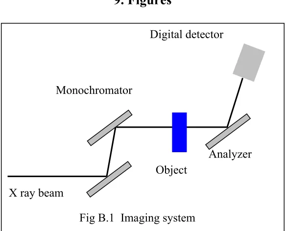
for diffraction enhanced imaging. Figure B.1 shows a schematic diagram of the data

acquisition system for DEI. The plane polarized white beam of synchrotron radiation from

an electron storage ring is Bragg reflected by a pair of monochromator crystals of silicon.

The Bragg angle of the monochromator determines the wavelength (or the energy) of the

reflected photons and thus the wavelength is tunable. Because of the nature of the

selects about a 1mm high beam to pass horizontally through the object to be imaged. The

beam transmitted through the object contains contributions from photons that were not

absorpted in the object, but also those which were diffracted, scattered or refracted by the

object. The latter three contributions typically will degrade the image quality in a

conventional radiograph. For DEI, another Bragg crystal tuned to the wavelength of the

incident beam is placed between the object and the detector. This crystal eliminates

virtually all of the scattered (coherent and incoherent) and diffracted photons from the

detected image. Because of the small but finite width of the rocking curve (reflectivity of

the crystal as a function of the Bragg reflection angle) of the analyzer crystal, and the fact

that refraction angles for x-ray photons are extremely small and fall within the width of the

rocking curve, the detected photons will contain contribution from refraction in addition to

x rays that are transmitted straight through the object. Refraction effects occur primarily at

the boundaries of embedded structures which have different indices of refraction. Thus, if

refraction contribution could be separated from the straight through contribution, the former

could display the valuable information that will delineate the boundaries of even minute

structures in the object.

The DEI methodology developed by Chapman, et al [1] does such separation of the

detected signals into an ‘apparent absorption image’ (actually the image from direct

transmission) and a ‘refraction image’ which correlates to the gradient of the refractive

index along the path of the x rays through the object. To facilitate this, two images of the

object are recorded on the digital recorder: one at an analyzer angle that is slightly greater

than the peak angle of the rocking curve (hereafter called ‘the higher side image’) and one

image’). According to Chapman, et al [1], the intensity diffracted by the analyzer set at a

relative angle θi from the Bragg angle θB where θB + θi is the angle between the incident

beam and diffraction planes and is given by

Ii=IRR( θB ± θi)

where Ii is the intensity at relative angle θi from Bragg angle θB, IR is defined as the portion

of the incident beam which has only been affected by refraction and attenuation by

absorption and extinction, and R(θ) is the analyzer reflectivity function at angle θ. R(θ) is

the function that describes the rocking curve.

By Taylor expansion, the intensity of the images taken on the lower side (θL) and

the higher side (θH) of the rocking curve are approximately

      _{+ ∆}

= L _z

L R L d dR R I I θ θ θ θ ) ( ) (       _{+ ∆}

= H _z

H R H d dR R I I θ θ θ θ ) ( ) (

where IL and IH denotes beam intensity at the lower and higher sides of rocking curve. Note

that R(θ) is written in a two-term Taylor expansion for the expressions above.

These two equations are solved for the intensity composed of apparent absorption, IR, and

for the refraction image angle, ∆θz, the angle through which x rays are refracted in the

z-direction in traversing the object. These solutions are

( )

( )

( )

( )

Typically, the lower and higher side images are taken at the half-widths of the rocking

curve which makes R(θL) = R(θH) = 0.5 with the peak reflectivity normalized to 1.0 and

because of the symmetry of the rocking curve around the peak,

( )

.

Thus, IR = (IL + IH) and ∆θz =

] [ ] [ dR/d 5 . 0 L H L H I I I I + − θ

∆θz provides the distribution of angles of refraction in the z-direction and it is not

the signal intensity due to refraction. The refraction signal intensity, Ir, is expressed by

IR(dR/dθ) ∆θz and hence proportional to (IL - IH) assuming that dR/dθ, the slope of the

rocking curve, is a constant at the high side and low side angles at which the two images

are measured. Note that simple addition and subtraction of the lower side and higher side

images can yield IR and IR∆θz images. We refer to the IR image as the “apparent absorption

image” and Ir image as the “refraction image”. Chapman, et al have always used IR and ∆θz

images in all of their work. Although ∆θz contains refraction information, we will be using

IR∆θz for the refraction images in this work because of reasons discussed later in Chapter 4.

It is possible to perform a further survey of the DEI modality by reviewing the

references quoted in the paper by Chapman, et al. Next, some of the important papers that

showed that DEI can reveal considerably more details in biological specimens than

conventional radiography are introduced. The papers, “Human breast cancer specimens:

diffraction-enhanced imaging with histologic correlation - improved conspicuity of lesion

contrast mechanisms in breast cancer specimens” [L.7] show that DEI can reveal

considerably more medically relevant details of breast tissue samples when compared with

standard radiography.

In addition to the research at the U.S. synchrotron laboratories, investigation of

phase contrast imaging are being carried out also at all of the major synchrotron light

centers in Europe using synchrotron x-rays, for example, [L.8] and in Russia [L.9].The

Russian work originated independently of the studies elsewhere using standard x-ray tubes

and therefore took prohibitively long times for data accumulation. Although these studies

have produced interesting results, the method of separating the absorption effects from the

refraction effects originated in the U.S. with the extensive work at the National Synchrotron

Light Source (NSLS) at Brookhaven National Laboratory and this method is now used

around the world.

2.4 Diffraction Enhanced Computed Tomography (DECT):

The first publication and so far, the only formal journal paper reporting on generating

tomographic reconstructions from DEI images is the paper by Chapman, et al [2]. This

work was carried out at NSLS using cylindrical acrylic phantoms with vertical and oblique

holes filled with oil. In this paper, the following four conclusions are derived. Firstly,

DECT projections are complete sets and thus can be reconstructed conventionally.

Secondly, the separation of the refraction image from the other image components is

complete for material with little small-angle scattering, such as oil and acrylic. Thirdly, the

refraction image contrast is proportional to the gradient of the refractive index. Finally,

and the theoretical refractive index results. The absolute values agree within 20%. This

thesis is a follow-up of the work reported in [2].

Preliminary work on a more exhaustive and versatile approach to DECT, known as

Multiple Image Reconstruction (MIR) is progressing at the laboratories of Chapman and

colleagues at the Illinois Institute of Technology [D. Chapman, Private communication,

(2002)]. MIR CT is capable of providing images of four x-ray parameters instead of two

(apparent absorption and refraction) in standard DECT. However, for clinical uses, MIR

CT images may turn out to be too difficult to interpret and use at least until the radiology

community gets attuned to viewing such data. Also, many images have to be acquired along

the rocking curve in doing MIR CT and radiation dose accumulation could become a

serious issue.

3. Experimental Methods

All of the data for this thesis were acquired at NSLS, Brookhaven National Laboratory

(BNL), using the X15A beamline. The first experiment was in December 2002. The main

objective of this experiment was to obtain two-dimensional DECT image of Lucite

phantoms and examine the characteristics of DECT images and the choice of the most

appropriate filter for backprojection. The second experiment was performed in the X15A

beam in February 2003. The aim of his experiment was to obtain three-dimensional images

of another Lucite phantom.

3.1 The DEI system at the X15A Beamline:

Figure E.1 shows schematically the experimental setup for DEI data acquisition at beamline

X15A. The Bragg angle of the monochromator selects the wavelength of the x-rays to be

used from the white synchrotron radiation beam. The monochromator and analyzer crystals

are both positioned on a large granite block, 0.375 m wide, 0.3 m tall and 2.1 m long. The

block is isolated from vibrations of the floor by rubber pads and vibration-insulating

composite plates placed under the legs of the steel frame that supports the block [e1]. The

monochromator is positioned inside a steel tank, sitting on the granite block and

mechanically isolated from the beamline pipe by an air gap of 2cm. To reduce the rate of

ozone production, the lower part of the x-ray spectrum is essentially eliminated using a 1

mm thick aluminum filter positioned downstream of the beamline’s beryllium window.

The sample scanning stage and shutter are placed on a platform positioned on a second

steel frame which is directly supported by the floor. Thus, the stage and the shutter are

. The X-ray energy was set to 40 keV and the maximum ring current was 178 m A.

X15A is a standard NSLS bending –magnet beamline. The fan beam is 130 mm wide at the

entrance to the experimental hutch, which is 16.3 m from the source. The useful height of

the fan beam is about 2 mm where the intensity falls 20 % below the flat top. The aperture

of the fan beam used for the experiment was 1.7 mm high and 128 mm wide. The x-ray

storage ring operated at 2.80 GeV energy.

Thomlinson, et al developed the monochromator and analyzer system for DEI in the

planar mode [e2], [e3], [e4]. It employed a two-crystal Bragg-Bragg monochromator using

a silicon [1 1 1] reflection for both crystals. The monochromator was placed inside the

stainless steel tank with helium at atmospheric pressure to prevent corrosion of its

components by ozone. Each crystal was 10mm thick and 150mm wide, with strain relief

cuts at 10mm from the ends of the crystal. Thus, the useful width of the crystal was 128

mm. The first crystal was 60 mm long along the beam’s direction, and the second one was

90 mm. The larger length of the second crystal allowed a long range of energy change

without requiring adjustment of the distance between the two crystals.

The monochromator is a box type design with a vertical offset of 1 cm between the

two crystals [e4]. The first and second crystals are mounted on the bottom and top plates of

the box respectively. Each crystal is mounted on kinematic mounts for adjusting the Bragg

and analyzer angles, and is supported on the back side by three balls placed under the strain

relief region, and secured on the front side by clamps. The box is mounted on a cradle, so

that the middle of the first crystal surface is at the center of rotation. Because of its

simplicity, the box type design is especially resistant to vibration. The instability of the

thermal equilibrium. This instability was assumed to be mainly caused by thermal drifts.

The thermal equilibrium was reached in about 5min after the white beam was first put on

the monochromator crystals. The analyzer crystal is of the same kind as the second crystal

of the monochromator but used the [3 3 3] reflections of silicon. The Bragg angle of crystal

is controlled by a tangent arm of 1m length, driven by a linear translator of resolution 0.1

µm. This arrangement provides an angular resolution of 0.1 µradian, which allows the

analyzer to be tuned at a precision angle equal to 1/30th of the full width at half-maximum

of the rocking curve. The tangent arm is supported by the same granite block that supports

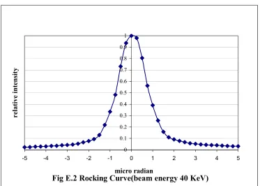
the monochromator. Figure E2 shows the silicon [333] rocking curves of the analyzer

crystal at 40 keV.

3.2 Data acquisition:

The digital detector was a Shad-o-box x-ray camera (Rad-icon Imaging Co. Ltd.) and the

data acquisition system (DAS) was interfaced with a Dell computer. The x-rays detected

by the digital detector in each pixel was transferred to the DAS and the data size was

reduced with IDL computer softwareby cutting out redundant pixels which did not include

any important information for data analysis. The raw data had a dimension of 2048 × 1024

pixels and it was reduced to the data size 2048 × 50. Since the height of x-ray beam is 2.5

mm, there was no important information seen by the detector except over this range. The

detector resolution was 50 µm. Therefore, 1mm is equal to 20 pixels.

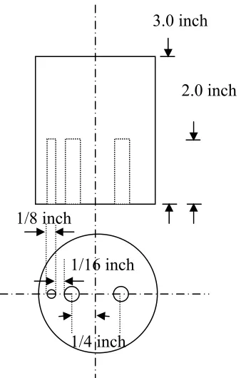
Two Lucite phantoms were used for the first experiment. One was prepared at North

Carolina State University (phantom A) and the other was prepared at BNL (phantom B).

the Phantom B was a lucite rod placed obliquely inside a hollow Lucite cylinder. Figure

E.3 shows the design of phantom A and Figure E.4 shows the design of the other phantom

B. The diameters of the channels for the phantom A were the following: 1/8 inch, 1/4 inch

and 1/4 inch. All of these channels were parallel to the phantom axis. The embedded

Lucite rod inside phantom B is 12.74 mm in diameter and placed at a tilt angle 21.5 degrees

with respect to the phantom axis. The reason that only phantom B was used in this thesis is

that to produce diffraction enhancement, the channels must not be parallel to the z-direction.

The channels in Phantom A are all vertical and hence no DEI could be done on it.

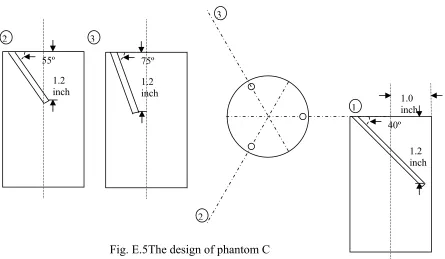
In the second experiment in February 2003, phantom C was prepared for obtaining

three-dimensional reconstruction data. The design of phantom C is shown in Figure E.5.

This phantom has three slanted channels with 1/8 inches diameter. These three channels

have angle of 40, 55 and 75 degree measured from top surface of the phantom. The

diameter of phantom is 2 inch.

Two sets of DEI scans were performed for each phantom by fixing the analyzer at a

specific angle and rotating the sample stepwise through 360º at 1º increment. In one set, the

phantom was filled with water and the other set, the phantom was empty. There are two

reasons for preparing these sets. First, the phantom, which was empty, was used to check

experimental set up accuracy, digital filter kernel size and other parameter adjustments.

This phantom should produce images which can be reconstructed with two parameters,

mass attenuation coefficient and diffraction enhanced signal. Second, the phantom, which

was filled with water, was used to see pure diffraction enhancement signal. Due to the

nearly equal values of mass attenuation coefficients of water and Lucite, the reconstructed

projections were acquired from the same sample with the analyzer angle tuned to -0.8 µrad

and 0.8 µrad from the peak and the sample rotated through 180 one-degree steps. The

FWHM of rocking curve at 40 keV x-ray energy is shown in Fig. E.2.

In each set of scans, three types of data were collected; these were background, air

and actual image. The background image was for obtaining information about detector

artifacts. Therefore, x-rays were not projected. The air image was for obtaining information

about attenuation from air. Therefore, x-rays are projected to the detector without phantom

in the beam. 20 sets of the background and air images were taken. Averaged values for

these were used to analyze data as described in the next section. The actual image is for

obtaining information about the phantoms. 360 images at 1 degree intervals were taken.

While performing experiments, the electron ring current of the synchrotron was in the range

between 215.3 and 184.8 mA.

All scans were controlled by a DEC Alpha computer with a program modified for

the CT experiment. The program obtains from the user data such as the type of scan and

the analyzer positions. Then, it performed the scan by controlling the stepping motors that

rotated. The program also acquired readings from the ion chamber current throughout the

4. Image Analysis and Reconstruction

In this chapter, the way we combined DEI and CT will be described. The manipulation of

order of these two can affect image quality. Therefore, it should be performed in the

appropriate order.

4.1.General Proceduresfor Image Analysis and CT Reconstruction:

As discussed earlier the experimental data for reconstruction of the two 2-D CT images of

apparent absorption and refraction consist of the 180 projections taken at the lower and

higher sides of the rocking curve and corrected for beam non-uniformities and air scattering.

The block diagram in Fig. I.1 shows the general procedure for construction a CT image of

the lower side or higher side data. The data sets are corrected for any non-axial rotation of

the object. They are then filtered and back projected.

Fig. I.2 shows the higher side and lower side CT images of Phantom B. Note that

absorption and refraction components are present in both images. The refraction effects are

visible at the boundary of the Lucite rod embedded within the water. However, the black

and white regions at the boundary of the rod are reversed in the two images. This is due to

the reversal of the polarity of the refraction signals in the high and low side images as seen

from the line scan profiles. The boundary between the water and the outer cylindrical

container shows almost no refraction since that boundary is vertical and the there is no

4.2 Separation of theAbsorption and Refraction Components:

The objective of DECT is to do tomographic reconstructions of the apparent absorption

image and the refraction image. Since this separation of components is peculiar to DECT

and unlike the case for conventional CT, question arises as to when this separation by the

addition/subtraction procedure (discussed in Section 2.3) should be performed during the

data analysis. There are three possible options (see Fig. I.1 also):

1. Separate the two components immediately after the raw projection data taken on the

higher and lower sides have been corrected for air scattering, beam non-uniformity

and non-axial center of rotation and then reconstruct the CT images of these

components using filtered back projection procedure. The absorption image is to be

reconstructed after a logarithmic transformation but the refraction image is to be back

projected without the transformation.

2. Prepare the filtered sinograms of the higher and lower sides after logarithmic

transformation of the corrected data as in the original program of Mark Rivers for

conventional CT and then perform the addition/subtraction step. The added and

subtracted data sets are then reconstructed by back projection.

3. Reconstruct the higher and lower side CT images after logarithmic transformation to

produce images like the figures associated with section 4.1, then perform the

addition/subtraction procedure on these two CT images on a pixel-by-pixel basis.

The three options described above are indicated by their corresponding numbers in

Fig. I.1. Of these, Option 2 is a clearly invalid procedure since the addition/subtraction

procedure is done on logarithmically transformed intensities of the signals and there is no

all of the absorption and refraction CT images from Phantoms B and C displayed a general

halo artifact which led to the recognition of the invalidity and abandonment of this

procedure for subsequent analyses. We will not discuss this procedure any further and we

will focus on Options 1 and 3.

Results of options 1 and 3 will be presented in Section 5. Now we wish to proceed

to the details of constructing sinograms and determining the center of rotation of the

phantom from the projection data.

4.3 IDL Code for CT Reconstruction:

In this section, the mathematical basis about Computed Tomography is briefly mentioned

ant actual calculation using IDL is discussed. For CT reconstruction, backprojection

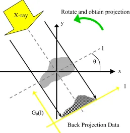
algorithm was used. Fig. I.3 shows the schematics of simple back projection. X ray is

projected to the object from a certain direction and an intensity profile is recorded at the

other side. The l-axis denotes width of beam or detector pixel position. Gθ(l) denotes

intensity profile or back projection data. This Gθ(l) can be mathematically expressed as

equation below;

∫∫ + −

= f x y x y R dxdy

l

G_θ() ( , )δ( cosθ sinθ )

This equation says that line profile Gθ(l) at position l can be obtained by summing up the

mass attenuation effect by function f on the line R. Where R is any line parallel to the x ray

direction. By taking this data from 0 to 180 degrees, sinogram can be obtained. Simple back

projection has intrinsic artifact, called 1/r artifact. Therefore, removal of this artifact is

important. To perform this, Shepp Logan filter was used for this research. The

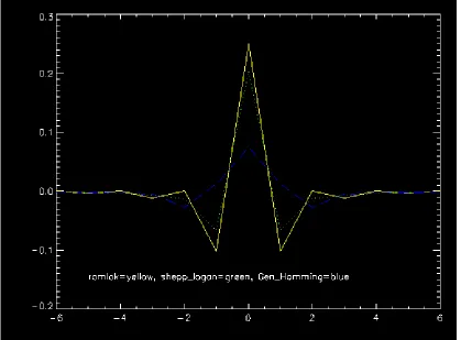
) 1 4 ( 8 ) ( , 0 2 , 4 sin ) ( 2 2 − − =      <       = k B k h otherwise B B H SL SL π π ω ω ω ω

HSL denotes Frequency domain and hSL donates mathematical form in the spatial domain.

Lam Rak filter has mathematical form of HLR=|ω|. Lam Rak is a high pass filter and causes

oscillations in the frequency domain. This causes ringing artifacts in an image. Please note

the difference between, HSL and HLR. Fig I.4 and Fig I.5 shows plots of these filters and of

Gen Hamming window. The mitigation of oscillation in spatial domain with Shepp Logan

and Gen Hamming windows can be seen.

Interactive Data Language (IDL) software was used to perform all of the image

analysis, CT reconstructions and graphic visualization. IDL version 5.5 is a specialized

fourth-generation language providing a framework that includes functions and tools for

scientific computing and visualization. Transforms such as Riemann sum or Radon

transform, as well as digital filtering are performed easily using IDL. Practical IDL

programming [I.1] and IDL Programming Techniques [I.2] are good books to understand

basic procedure to write IDL codes. The IDL code that was used to prepare sinograms and

reconstruct tomographic images from the raw data files is attached in Appendix. The basic

summaries of what the code does are given below. There are three types of raw data for

each set of images; background, air and actual projections. Twentysets of background and

air images were averaged and used to produce the normalizing image for calculating the

actual image that is free of beam non-uniformities and air scattering. Here, the normal

image was subtracted from the detector image of the object, and then divided pixel by pixel

by this normalizing image. These were stored as raw tomography images. The detector

had a pixel size of 50 µm and there are 2048 pixels along each row. Since this data set was

too large for data analysis, the image size is reduced by factor of four using the Expand

command of IDL. The expand procedure shrinks or expands a two-dimensional array using

bilinear interpolation. Therefore, there were a total of 512 pixels and each pixel

corresponded to 200 µm. The raw tomography projections were transformed to sinogram

using Sinogram.pro procedure, which was written by Mark Rivers [I.3]. This procedure

mainly does the following. Please note that this procedure was skipped for generating the

refraction image of option 1. First, it averages the air values on the left and right hand sides

of the input. These averaged values were used to adjust horizontal intensity distribution of

the beam. The beam intensity is adjusted linearly. Second, it takes the logarithm of

input/air ratio; the output = - log(input/air). Please note that air images correspond to initial

intensity of the x rays and the input corresponds to actual images, which contains

information about the object. Therefore, the output corresponds to line integral of the

object. Finally, it calculates the center of gravity of the image and shifts the actual image

center to match the center of image by using the center of gravity. The center of gravity of

image at each row was calculated by the equation below.

∑

∑

Here, COG is center of gravity, I(i, j) is the intensity of the pixel (i,j), (m,n) is dimension

of sinogram; n corresponds to rotation angle and m corresponds to image width. Therefore,

the value of n should be 179 or 359 generally.

The numerator is the moment of each row of the image and the denominator is the

sum of intensity of at each rotation angle, i. The COG of image draws a sine curve. By

taking the average of the max and minimum value of COG, the actual rotation axis is

estimated. To fit this sinusoidal curve, and estimate the center of gravity of image, the

Curve-fit procedure is used. The shifting of raw images to match with the center was done

using a routine called Poly_2D which can shift the image by fractional pixels. Since DEI is

a phase contrast method and enhances the edge contrast, the Shepp Logan filter was chosen

as the digital filter. The raw sinogram was filtered with Shepp Logan filter by calling

tomo_filter.pro procedure. This procedure contains a choice of three major types of high

pass filters; Ram-Lak, Shepp Logan and Gen Hamming window. From this filtered

sinogram, tomography images were reconstructed by using Riemann sum routine, which is

one of the back projection methods of IDL. What the Riemann sum routine does is to

smear the 180 sets of back projections from each angle. Therefore, the manipulation of

image with filters is important for removing halo artifacts or 1/r artifacts that arise from

simple back projection. For example, the Shepp Logan filter enhances high frequency

information while reducing low frequency information in Fourier domain. Please note that

high frequency corresponding to sharp transition of image or edge and low frequency

correspond to smoother transitions in image. This characteristic of the Shepp Logan filter is

clear from Fig. R.1.13 and Fig. R.1.14 which are line profiles of an image with and without

5. Results and Discussion

In this Chapter, we start with the results of a 2-D reconstruction of DEI images and then

proceed to present the results of the three-dimensional visualization of images that were

generated from the 2-D slices. All of the results used projection data for Lucite phantoms B

and C.

5.1 Two-dimensional Slice Reconstruction Using Option 3:

Figure R.1.1to R.1.6 demonstrates how images are reconstructed from raw data. Figure

R.1 shows a slice of the raw projection data which was detected by the digital detector.

Several scratches can be seen everywhere in the projection. These detector artifacts were

removed by dividing the raw image by the normal image. This raw projection data covered

a height of 2.5 mm or 50 pixels. The middle row of pixels from this slice was chosen from

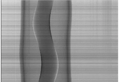
the raw projection data slice for each angle of rotation of the object. Figure R.1.2 shows

raw tomography data of Lucite B at lower side of rocking curve. All images discussed

below were obtained at the lower side of rocking curve, unless mentioned otherwise. Here,

each row of arrays stands for a projection angle (0 degree to 360 degree from top to

bottom) or y-direction and column of arrays stands for intensity or x-direction. In this

figure, the Lucite phantom shows strong refraction signals due to the sharp gradient of the

refractive index between Lucite and air. The stripes in the y-direction are because of beam

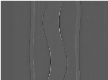
intensity fluctuations. Figure R.1.3 shows the sinogram of Lucite B, where the raw

tomography data is modified to a sinogram by calling the sinogram routine. Therefore, the

center of gravity of this image is matched to the middle of column array and “padding” can

adding some pixels on left side, whose values are same as the very left pixel in the original

image and some pixels in the image were trimmed, since the image was shifted to right.

Also, logarithm of raw tomography data is taken to change the value to correspond to mass

attenuation coefficient. The vertical line which shows up on the left side of the phantom is

a detector artifact. Figure R.1.4 shows the sinogram of Lucite B with Shepp Logan filter,

which enhances the clarity of the edges. Kernel sizes of 10, 15, 30, and 40 were tried and

the kernel size of 30 was chosen subjectively based on the observed image quality. A

kernel size of 30 is recommended for conventional usage for back projection.

Figure R.1.5 shows reconstructed image with the Shepp Logan filter. The center of

rotation is automatically calculated by the sinogram procedure, but the image shows that it

is a little off from the true center of image. This is because of noise in images and

asymmetry of the DEI signal. This asymmetry is discussed later. Figure R.1.6 shows

reconstructed image without filters. This image shows that simple back projection causes

blurring. Comparison of Figures R.1.5 and R.1.6 is interesting for understanding the effects

of Shepp Logan filter. At the corners of Figure R.1.5, ray artifacts show up, but this can

not be seen in Figure R.1.6. In the very center of Figure R.1.5, a small circle or dot can be

seen because of a detector artifact. Also, a semicircular arch can be seen right below the

Lucite image. These artifacts are not seen in Figure R.1.6. Thus, Shepp Logan filter does

enhance edges in the image, but exaggerates noise at the same time. It should be noted that

filter choice is usually a subjective factor and might cause loss of critically important

information.

Figure R.1.7 to R.1.14 shows line profiles of raw tomography data, sinograms and

signals. Figure R.1.7 shows a line profile of raw tomography data at y = 169, where DEI

signals disappear. Please note that y-direction is the angle of rotation for sinograms. DEI

signal occurs due to differences of refractive index in the z-direction which is normal to the

x-y plane or the reconstructed image. Figure R.1.8 shows a line profile of the sinogram at

the same point. The center of column and the center of rotation are matched. Due to this

manipulation, the image is shifted to the right and some pixels are padded in the left side of

image. Theoretically, the embedded cylindrical Lucite rod should have an elliptical shape

for its back projection. So this results matches with theoretical back projection profile fairly

well. Figure R.1.9 shows a line profile of sinogram at the same point with Shepp Logan

filter. Noise is exaggerated as previously discussed. The negative signals detected here is

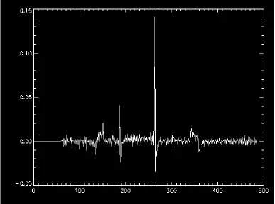
because of Shepp Logan filtering and not because of the refraction signal. Figure R.1.10

shows a line profile of raw tomography data at y = 255, where the refraction signal appears

to be the strongest. Figure R.1.11 shows a line profile of the sinogram at the same point.

The absolute values of intensity of the refraction signal at both of left and right side should

be the same theoretically. However, asymmetries of signals are detected and cause the

center of rotation to be slightly different from the center of image. Figure R.1.12 shows a

line profile of sinogram at the same point with Shepp Logan filter. The strong signal due to

refraction is observed. However, the asymmetry of DEI signals is exaggerated as well.

Figure R.1.13 shows a line profile of the reconstructed image with Shepp Logan filter. This

result shows the effectiveness of this filter for this phantom in that all signal intensities

from Lucite are fairly flat. The maximum noise of back ground is about 0.3 and the

maximum DEI signal is about 3.9. Therefore, SNR is 13 in this case. Figure R.1.14 shows

obvious when compared with Figure R.1.13. Since Figure R.1.14 is from simple back

projection, 1/r artifact can be seen.

Figure R.1.15 to R.1.21 shows the results obtained at the high side of the rocking

curve. Figure R.1.15 shows the raw tomography data and Figure R.1.16 shows the

normalized data. As discussed previously, the raw tomography data wasdivided bythe

normal data and converted to a sinogram after taking logarithm. Figure R.1.17 and Figure

R.1.18 show the sinograms of Lucite B at higher side of rocking curve without filtering and

with filter, respectively. One of the most significant differences between images of the

lower and higher side of rocking curve is that the dark and bright parts are flipped. This is

because the rocking curve has different gradients at lower side and higher side. Therefore,

the same amount of refraction at each side causes opposite DEI signals.

Figure R.1.19 shows the reconstructed image. The dark and bright parts in the

image are different from the result for the lower side of rocking curve (Fig R.1.5). It should

be noted that the mismatch of center in this image is small compared with that of Fig R.1.5.

The line artifact which showed up at the edge of the embedded Lucite is smaller. Figure

R.1.20 and R.1.21 show line profiles of raw tomography data and the sinogram respectively.

The DEI signal is fairly symmetric. This causes the difference in the images of Fig R.1.19

and Fig R.1.5. The center of rotation is estimated by calculating intensity times position at

each row or angle of sinogram. Since the total mass attenuation by the Lucite is the same,

total intensity of each column of sinogram should be same. However, the center of gravity

moves as a sinusoidal curve because of the non-axial rotation of the phantom. It should be

noted that refraction signalcannot be used to estimate the center of image by this method,

is symmetric, the sum of DEI signal at each row is equal to zero. Therefore, the center of

rotation can be estimated by the same method as with conventional tomography data.

For the option 3 method of separating the apparent absorption image and the

refraction images, we add and subtract the CT images of the higher and lower sides of the

rocking curve respectively. We conjecture that the addition provides the absorption image

as specified by the theory of DEI presented in Section 2.3 and that the subtraction will give

the refraction image. The resulting absorption and refraction image for phantom B is shown

in Fig.1.22 and Fig. 1.23. Line scans through absorption and refraction at the location

indicated are shown in Fig.1.24 and Fig.1.25 respectively. Note that a line scan through

this image at the location of x=250 shows that the absorption signals from Lucite

attenuation is fairly flat. It is interesting to note that there is a small amount of refraction

effect evident in the absorption image. This is most probably coming from a slight drift in

the rocking curve during projection data acquisition which causes the higher and lower side

image angles to be slightly asymmetric with respect to the center of the rocking curve.

Since the angular settings are less than only one microradian above and below the center,

even a very minute drift will cause asymmetry and negate the assumptions made in the

theory regarding the reflectivity values of the analyzer crystal. Refraction image was

obtained by subtracting the higher side CT image from the lower side CT image. The

refraction image looks very clean and the line scan through the Lucite rod shows essentially

only the refraction signals at the boundaries.

To compare option 3 with option 1, the apparent absorption and refraction images of

phantom B using option 1 are shown in Fig. R.1.26 and Fig. R.1.27 respectively. Line

option 1 will be discussed in the following section. The biggest differences between option

1 and option 3 is that the refraction signal with option 3 reconstruction shows much larger

values than that of option 1. This is because we are taking logarithm for refraction image

with option 3. This fact shows that less absorption and highly refractive images are

vulnerable to error with the option 3 method.

In summary, option 3 appears to give clean CT images of apparent absorption and

refraction that show the expected results. But one might wonder why subtraction of the CT

images from the high and low sides of the rocking curve which were generated assuming

that the signals are comprised purely of exponential attenuation should produce such good

results for the refraction image; after all, the refraction signals do not follow any

exponential law. The reason appears to be the fact that on both sides of the rocking curve,

for this particular phantom, the signals are comprised almost through the whole phantom by

exponential attenuation and the refraction signals are localized just at the boundaries of the

embedded rod inside the phantom.

To verify this hypothesis, we simulated the projection data for a Lucite cylinder of

the same dimensions as the phantom, assuming just exponential attenuation (no refraction

effects). Fig. R.1.30 shows the comparison of line scans through the same projection for the

simulation and for the higher side data of the water-filled phantom B. The amplitude was

scaled to match the two sets of data. Note that the overall shape of the real image agrees

very closely with the simulation which ignored refraction effects. The minor differences

observed are likely due to the differences in attenuation coefficient between water and

Lucite and the refraction signals present in the real image. Also, the simulated image is free

dominated by exponential attenuation. This is also the case for the lower side data.

Therefore CT reconstruction of the higher and lower side data after logarithmic

transformation is valid and the subtraction ought to provide a good image of the refraction

signals.

5.2 Two-Dimensional Slice Reconstruction Using Option 1:

It is important to recognize that the validity of Option 3 is demonstrated above only for a

simple phantom. In a complex biological sample with a very high degree of heterogeneities

where refraction might be present throughout the specimen, Option 3 might not be a valid

method. Option 1 appears to have a better theoretical basis than Option 3. In this method,

the separation of the two components by the addition/subtraction procedure is performed on

the projection data (raw tomography data) and not on the CT images of the higher and

lower sides. The absorption component projections are reconstructed as in conventional CT

after logarithmic transformation, but the refraction projections are reconstructed by filtered

back projection without taking logarithms.

Figures R.2.1through R.2.8 demonstrate how images are reconstructed from raw

data with using option 1. First of all, raw tomography data of lower side and higher side

are added/subtracted to obtain raw tomography absorption and refraction data. Absorption

and refraction raw tomography data are shown in Fig. R.2.1 and Fig. R.2.2, respectively.

The apparent absorption image looks like one cylindrical object. The inside rod Lucite can

not be seen. Please note that digital addition is a mean filter and subtraction is a high pass

filter. Therefore this mathematical procedure imposes filtering to raw tomography data or

sine curves can be seen. This caused artifacts in refraction reconstructed image, which will

be shown in the later of this section. These raw tomography data were converted to

sinograms. Absorption and refraction sinograms are shown in Fig R.2.3 and Fig R.2.4,

respectively. For the absorption image the conventional method which described in

previous section was used. Therefore, the absorption image was converted to sinogram, or

mass attenuation component. It is performed for the refraction image to shift the refraction

image to match the center of the image and the rotation axis. Please note that logarithm

was not taken for the refraction image. These absorption and refraction images were filtered

using Shepp Logan filter and shown in Fig R.2.5 and R.2.6 respectively. In Fig R.2.5, two

vertical lines can be seen. These are boundary of the digital detector. In Fig R.2.6, square

shape can be seen on the left side of image. This part showed up because of patting due to

shifting the image to the right. This padding caused a big circle-like artifact in the

reconstructed image, which will be shown later. Figure R.2.7 and R.2.8 shows

reconstructed apparent absorption and refraction images respectively. Figure R.2.9 and

R.2.10 shows line profiles at x=250 of those. In Fig. R.2.7, refraction signal still can be

seen, but the image has high quality. In Fig. R.2.8, you can see artifacts outside of the

Lucite. However, outside Lucite is not our concern. Fig. R.2.9 shows slopes outside lucite.

This is intrinsic artifact caused by Shepp Logan filter. The boundary between cylindrical

Lucite and outside air is clear. Fig. R.2.10 shows four big peaks. Two of those outside are

signal from boundary between air and Lucite. These signals are strongest due to the large

refractive index difference between air and Lucite. The two inside signals are signals from

the boundary between water and the inner Lucite rod. Other small signals are those from

A lot of time was spent using option 2 reconstruction method through this research.

However, we found that it produced unexplainable artifacts. Option 3 produces good

images. Through even further in-depth investigation about reconstruction methods, it was

found that option one gave the best result.

5.3 Three-dimensional reconstruction of Phantom C:

In this section, three-dimensional reconstruction of apparent absorption images and

refraction images from the transverse multiple slice data which were acquired on the

second phantom (phantom C shown in Fig. E.5) with the oblique air holes will be presented.

First, two-dimensional images or CT slices of absorption and refraction images obtained

using option 1 are shown. These CT images were then stacked up to compose a

three-dimensional image. The final result had the dimension of (x,y,z)=(487,487,40). Here, the

x and y values denote the transverse image size in pixels and the z-value denotes the height

of image in pixels. Note that the height covers only 2 mm (40 pixels) because of some

difficulties which were encountered with the stability of the synchrotron beam during the

second set of experiments at NSLS. The image is shrunk by factor of four in the x-y plane

using the expand command of IDL. Therefore one x- or y-pixel size corresponds to 200 µm.

In the vertical direction, there is no reduction of pixel size and one pixel corresponds to 50

µm. Using this array, transverse slices of absorption image and refraction image were

obtained. Line profiles of refraction image and absorption image were also obtained, where

line profile means one row or column of image plane(x-y plane). Finally, three-

dimensional voxel projection images of absorption and refraction images will be shown.

signal. However, the voxel projection images show some difficulties of DEI in producing

three-dimensional voxel projection.

Figures R.3.1 and R.3.2 show the CT reconstruction of radial refraction and

apparent absorption images, respectively. Let us label the holes in upper left, center and

lower right as 1, 2, and 3, respectively. The slices for absorption images were taken at the

same locations. Fig R.3.1 shows strong noise outside Lucite. This is caused by beam

intensity being not automatically adjusted for the refraction image. However, the region

outside of the Lucite is of no interest. Fig R.3.2 shows some contamination from refraction

signals within the absorption image. As with the previous results on phantom B, there

appear to be some contamination from refraction effects in the absorption image and vice

versa in the refraction image. This was likely caused by slight drift of the angular position

set on the rocking curve of the analyzer crystal while performing the data acquisition. Since

the angular settings are at only ± 0.8 µrad from the peak of the rocking curve, even a very

slight drift in the rocking curve during the data acquisition will negate the cleanliness of the

refraction and absorption images.

Figure R.3.3 and Figure R.3.4 show the transverse slices of the refraction image and

the apparent absorption image respectively. These images show that signals from the

gradients in the refractive index shows up correctly in the vertical cross section plane. The

reason for some gray scale difference in images is the differences in the refraction signal

strength in the images. For example, if an image has strong positive refraction signal, the

other pixels have relatively low values. Therefore, the image looked darker. (b.1) showed

the elliptical shape in the signal. This was caused by the fact that the slice was taken at near

asymmetry. This was caused by fact that the direction of hole and the transverse plane did

not go in the same direction. In Fig R.3.4, clear surfaces between channels and Lucite can

be seen, although these images include partial contamination from the refraction signal.

From (b.1) to (b.4), the signals from refraction are seen. However, these images showed a

clear edge, since apparent absorption image excludes scattering. Specifically, please note

that the holes and backgrounds have similar gray scale levels in each image.

For further discussion of image qualities, the line profiles of refraction image and

apparent absorption image are shown in Figure R.3.5 and Figure R.3.6 respectively. The

x-axis and y-x-axis in these figures represent pixel number from the left side of an image and

relative intensity. The signals from refractive index can be seen in Fig. R.3.5. The reason

why the edge of Lucite can be seen clearly is that the noise level dramatically increased

outside the Lucite. Please note that this profile is free from the absorption component.

However, Fig R.3.6 shows contamination from refraction signals and slight slope outside

Lucite. However, clear edge between Lucite and the outside air can be seen and channel 2

showed up clearly. This channel has almost identical value with outside air as expected.

Using the 2-D slices, three-dimensional voxel projection of refraction and apparent

absorption images were attempted . The results are shown in Figure R.3.7 and Figure R.3.8

respectively. Voxel projection assigns opacity according to intensity of each voxel. Figure

R.3.7 (a) shows the surfaces of channels since these signals include information on the

gradient of the refractive index. The non-uniformities within the holes are likely caused by

the roughness developed during machining of the holes. The reason that dark regions exist

which the difference of refractive index disappear in z-direction. Signals from refraction

reverse at this point from positive to negative or vice versa.

Fig R.3.8 shows the 3-D apparent absorption image. To obtain this image, the

procedures described below were performed. Since 3-D imaging here is just a procedure

for visualization, empirical adjustments as below could be made in order to make the

images visually acceptable. First, values outside of the Lucite were changed to zero and one

was added to this region. The median of Lucite intensity was calculated andthis value was

divided by two. This value was multiplied by the values outside the Lucite. According to

these processes, outside Lucite has a unique constant equal to the median of Lucite value

divided by two. The high opacity values were assigned to channels. Lucite was assigned

small opacity. The opacity for Lucite was set to one tenth of those of channels. The result