ABSTRACT
STRICKLING, HAYDEN LELAND. A Bayesian Hierarchical Model for Estimating Nutrient Export Rates in a Developing Watershed. (Under the direction of Dr. Daniel Obenour).
A Bayesian Hierarchical Model for Estimating Nutrient Export Rates in a Developing Watershed
by
Hayden Leland Strickling
A thesis submitted to the Graduate Faculty of North Carolina State University
in partial fulfillment of the requirements for the degree of
Master of Science
Civil Engineering
Raleigh, North Carolina 2017
APPROVED BY:
_______________________________ _______________________________ Daniel Obenour Emily Berglund
BIOGRAPHY
ACKNOWLEDGMENTS
I’d like to thank my advisor Dr. Daniel Obenour for his guidance and instruction. I’ve
TABLE OF CONTENTS
LIST OF TABLES ... vi
LIST OF FIGURES ... vii
INTRODUCTION ... 1
METHODS ... 8
Study Area ... 8
Estimates of Annual TN Loads ... 10
Uncertainty Analysis for Load Estimates ... 11
Nitrogen Source Inputs ... 13
Nitrogen Retention ... 16
Bayesian Model Formulation ... 18
Prior Distributions ... 21
Performance Assessment ... 23
RESULTS ... 24
Annual TN Loads ... 24
Model Parameterization and Performance ... 25
Nutrient Loading Source Apportionment ... 31
DISCUSSION ... 34
REFERENCES ... 41
APPENDICES ... 50
Appendix A. NWALT Land-Use Classifications ... 51
Appendix B. Probabilistic Comparison of Parameter Magnitudes ... 52
Appendix C. Modified Export Coefficients Including the PIC for Each Source ... 53
Appendix D. Coefficient of Variation (CV) Values from the WRTDS Uncertainty Analysis... 54
Appendix E. Mean Annual TN Loads from Point Source Dischargers ... 55
Appendix F. Land Use Change Maps ... 56
Appendix G. WRTDS TN Estimates for Stations in Each River Basin ... 57
Appendix H. Percent TN Retention Map ... 59
Appendix I. TN Loading Rate Maps ... 60
LIST OF TABLES
Table 1. Parameters used in the model with their prior distributions ...22 Table 2. Mean parameter estimates with 95% credible intervals for models with priors,
LIST OF FIGURES
Figure 1. The North Carolina river basins used in this study: Tar Pamlico, Neuse, and Cape Fear ... 9 Figure 2. Nitrogen source data for each river basin (1994-2012) ... 15 Figure 3. WRTDS estimates of TN loadings at downstream locations in the CFRB,
NRB, and TPRB... 25 Figure 4. Posterior distributions of model parameters with prior distributions ... 28 Figure 5. Observed vs. predicted plots of incremental TN loadings using full model
with fixed and random effects, full model with fixed effects only, and cross validation with fixed effects only ... 30 Figure 6. TN loading contributions in the CFRB, NRB, and TPRM for 1994 and
2012, by source type ... 32 Figure 7. TN loading rates for the year 2002 and change in loading rate from 1994 to
INTRODUCTION
Hybrid watershed models typically characterize pollutant sources in terms of land-use export rates (kg/ha/yr), also known as export coefficients (ECs), which can be useful for forecasting outcomes of nutrient management or development scenarios. The EC concept has been effective in relating anthropogenic land-use practices to downstream water quality in past studies (Vollenweider et al., 1971; Norvell et al., 1979; Johnes, 1996), and in the development of Total Maximum Daily Load (TMDL) allowances (Mattson & Isaac, 1999). Often, ECs are estimated through field studies of small single land-use watersheds (Beaulac & Reckhow, 1982). These estimates, however, may not be available for a particular region or may not represent a mean rate for a basin-scale study where heterogeneity of land-use practices and characteristics exist (Shrestha et al., 2008). Hybrid models, on the other hand, can provide an estimate of mean loading rates over large regions through empirical estimation based on available water quality data, watershed characteristics, and land-use data (Alexander et al., 2004). Statistical approaches can also quantify uncertainty in EC estimates, which is important in assessing the reliability of model estimates for considering risk in watershed management (Reckhow, 2003; Xia et al., 2016).
understanding of the causes of adverse loading moments, which can inform more effect management strategies (McClain et al., 2003).
Few efforts have been made to include interannual variability in hybrid watershed models. Wellen et al. (2012) added temporally variable climatic variables as an additive component to the SPARROW regression and Xia et al (2016) included land-use change. In addition, both of these studies used dynamic parameter estimation, allowing relationships to vary over time. However, for hybrid models, precipitation has yet to be incorporated into the formulation of nutrient export, and the interplay between changes in land use and climate has received little attention. Since both precipitation and land use are primary drivers of interannual variability in nitrogen export (Haith & Shoemaker, 1987; Sinha & Michalak, 2016), their inclusion within the mechanistic formulation of hybrid models could improve our understanding of watershed loading dynamics.
Understanding temporal variability in watershed nutrient loading is particularly relevant for watersheds subject to changing land use practices. Our study consists of three such watersheds in eastern North Carolina: Neuse River Basin (NRB), Cape Fear River Basin (CFRB), and Tar Pamlico River Basin (TPRB). Estuaries in these basins have been subject to toxic algal blooms, hypoxia and fish kills in the past decades, resulting in diminished water quality, and their inclusion in the United States Environmental Protection Agency (EPA) 303(d) list of impaired waters in the 1990s (Paerl et al., 1998; Burkholder et al., 2006). The causes of impairment were identified as chlorophyll a level exceedance for the NRB and TPRB, and low dissolved oxygen (DO) levels for the CFRB, both attributed to up-stream nitrogen loadings (NCDEQ, 2017). As mandated by the Clean Water Act (Clean Water Act, 1972) for impaired water bodies, the North Carolina Division of Water Quality developed a Total Maximum Daily Load (TMDL) requiring point and distributed source total nitrogen (TN) loading reductions of 30% in the NRB and TPRB, relative to 1990-1994 base-line years (NCDENR, 1999; NCDENR, 1994). By 2008, however, the 30% reduction goal had not been achieved (NCDENR, 2009; NCDEQ, 2010).
1995 hog and chicken production increased 200% and 50% respectively in NC, prompting the implementation of a state-wide moratorium in 1997 on new hog operations, still effective to date (Cahoon et al., 1999; S.L. 1997-458, 1997). Chicken operations expanded steadily since the 1990s making North Carolina one of the nation’s top producers of chickens by 2012
lagoons from extreme weather can also contaminate surface waters, a concern especialy for the hurrican-prone regions of eastern NC (Burkholder et al., 1997).
Another potential driver of this increasing ON loading into NC estuaries is land-use activities such as agriculture and urban development, resulting from population growth nearly doubling from 1990 to 2010 in the three basins (U.S. Census Bureau, 2017). Urban development increases nutrient transport to surface waters through the destruction of riparian forested and wetland buffers, disruption of soils resulting in sediment transport of nutrients, and increased impervious development that accelerates nutrient wash-off from lawn fertilizers and pet waste (Lee et al., 2006; Reavie & Baratono, 2007; Hopkinson & Vallino, 1995; Hogan & Walbridge, 2007; Faulkner, 2004). Agricultural cultivation also affects water quality through transport of fertilizer inputs through ditches and sub-surface tile drains (Cambardella et al., 1999; Robertson & Vitousek, 2009) though agricultural cultivation has not increased substantially in the study area in recent decades. To investigate the relationship between land-use and nutrient loadings of dissolved organic nitrogen (DON) in the NRB, Osburn et al. (2016) matched water sample fluorescence tracers with that of various DON sources and found soil DON to be the dominant type in the NRB, just above chicken litter and street runoff. Soil DON likely comes from disruption of soils caused by urban development and leaching of nitrogen from agricultural soils during precipitation events (Osburn et al., 2016). Thus, the combined effects of urban and agricultural land-use practices could account for the increase in ON noted above.
export from distributed and point-sources in the NRB, TPRB, and CFRB. SPARROW model predictions for the NRB show a watershed nitrogen budget dominated by agricultural inputs from the lower part of the basin where shorter transport distances allow for fewer in-stream losses (McMahon et al., 2003). Qian et al. (2005) built upon this model by introducing a Bayesian hierarchical framework to test different model formulations and account for spatial autocorrelation of residuals and variability among watersheds. While providing useful estimates of nutrient delivery for this region generally reflective of conditions prior to 2000, neither of these models directly address precipitation variability and changing land-use practices, nor include CAFOs as potential sources of nitrogen.
METHODS
Model development involved several steps. First, annual loading rates for sub-watersheds were estimated from available TN concentration and flow data, and the uncertainty in these estimates were determined through sub-sampling. Next annual data for the TN sources used in the model were collected and aggregated for each sub-watershed. A basin-wide stream and water-body network was developed to account for TN retention and annual precipitation data was obtained for each sub-watershed to address the effect of precipitation on nutrient delivery rates. Next a non-linear regression model formulation was developed to relate TN source, stream and water-body network, and precipitation data to the estimated loading rates. Finally, the model was developed in a Bayesian-hierarchical framework that incorporates the uncertainty in the loading rate estimates, a random effects term grouped by sub-watershed, and the prior distributions of model parameters, obtained from the literature.
Study Area
USGS National Elevation Dataset (USGS, 2017) (Figure 1). The study period is 1994 to 2012, as limited by nutrient-source data availability.
Figure 1. The North Carolina river basins used in this study: Tar Pamlico (red), Neuse (blue), and Cape Fear (yellow). Darker shades outline the portion of each river basin used in
Estimates of Annual TN Loads
Uncertainty Analysis for Load Estimates
Uncertainty in WRTDS estimates was determined by relating error variance to sampling frequency at monitoring stations. This relationship was developed by sub-sampling at four stations, selected for having nitrogen concentration samples taken nearly every day over a span of at least 7 years. Subsampling of concentration data was implemented based on different sampling schedules: samples taken every two months, 1 month, 2 weeks, 1 week, and 4, 3, and 2 days. Samples were selected at random within a sliding window corresponding to each sampling schedule to simulate real-life variability in sample collection. For each sampling schedule, WRTDS was run 300 times (simulations) with a different randomly selected subsample used for each simulation. A 3-year half-window width was used in the WRTDS estimation, and annual loading estimates were taken from year(s) within 3 years from the start and finish of the simulation. The window width refers to the time-span for the distribution of weights used for the WRTDS regression analysis, where data outside this window will be assigned a weight nearly zero (Hirsch et al., 2010). Residuals were determined by subtracting WRTDS loading estimates based on subsamples from those obtained using the complete dataset. For each year (t) of each simulation, a coefficients of variation (CV) was calculated:
𝐶𝑉𝑡= 𝜎𝑡 𝜇𝑡
where 𝜎𝑡is the standard deviation of residuals, 𝜇𝑡 is the mean loading estimate (for a simulation in year t). Results from subsampling are shown in Appendix D, where CV values are plotted as a function of number of samples per year. A power function was fit to this distribution and used to estimate CV based on number of samples taken per year (R2 = 0.95):
𝐶𝑉𝑖,𝑡 = 0.9662 ∗ 𝑋𝑖,𝑡−0.783 (2)
where 𝐶𝑉𝑖,𝑡 is the coefficient of variation for watershed i and year t, and 𝑋𝑖,𝑡 is the number of
samples taken. Equation 2 was applied to calculate the CV for each annual WRTDS loading estimate for each of the 21 sampling stations used in this study. These CVs were then used to determine the standard deviation of each loading estimate, consistent with equation 1. The incremental error variance, representing the uncertainty in the change in loading across an incremental watershed, is calculated based on the relationship between two correlated random variables (Kottegoda & Rosso, 2008):
𝜎̃𝑖,𝑡2 = 𝜎𝑧,𝑖+1,𝑡2 + 𝜎𝑧,𝑖,𝑡2 − 2𝜌𝑖+1,𝑖𝜎𝑧,𝑖+1𝜎𝑧,𝑖 (3)
where 𝜎̃𝑖,𝑡2 is the incremental error variance for incremental watershed i and year t, 𝜎𝑧,𝑖,𝑡2 is the
WRTDS error variance for station i, 𝜎𝑧,𝑖+1,𝑡2 is the error variance for the upstream station to station i, 𝜌𝑖+1,𝑖 is the correlation of loadings between watershed i and the upstream watershed, 𝜎𝑧,𝑖+1 is the WRTDS standard deviation of station i, and 𝜎𝑧,𝑖 is the WRTDS standard deviation
Nitrogen Source Inputs
Three types of nitrogen sources were included in the model: distributed sources associated with land use, point-source dischargers, and CAFOs. Land-use data were acquired from the U.S. conterminous wall-to-wall anthropogenic land-use trend (NWALT) dataset for the years 1992, 2002 and 2012 (Appendix A) (Falcone, 2015). For the purposes of this study, land use classifications were aggregated into three general categories: developed, agriculture, and wild. Both low-use and low-use/conservation classifications were grouped into wild, and three classifications within production make up the agriculture group: Crops, Pasture/Hay, and Grazing Potential. The developed group comprises a range of land-use classifications
including low-, medium-, and high-density commercial, industrial, recreational, and residential areas. Land-use area for each of the three groups was calculated on the Hydrologic Unit Code (HUC 12) spatial scale. Land-use areas for years in between the NWALT datasets were calculated through linear interpolation.
Figure 2. Nitrogen source data for each river basin (1994-2012). Included are the area of distributed sources, Agriculture, Developed, and Wild (106 ℎ𝑎), chicken (108) and hog (106)
counts, and TN loadings from point source dischargers (106 𝑘𝑔 𝑦𝑟).
annual estimates for broilers and layers are only available from 2006-2012. Layer and broiler production counts for years preceding 2006 were estimated using 5-year census data with linear interpolation to estimate in-between years. Livestock densities were distributed across incremental watersheds by area-weighting. County level counts are the best available source of livestock data, since comprehensive CAFO records are only available after 2003 (J.R. Joshi, NC DEQ, personal communication, 2017). Nitrogen content of both chicken and hog waste was calculated using the 2017 North Carolina Agricultural Chemical Manual estimates of manure volume produced per animal per year and nitrogen content per volume. Broilers, layers and hogs were estimated to produce 0.19, 0.52, and 6.3 kg/animal/yr of nitrogen respectively (NC State University, 2016). In general, there was a dramatic increase in livestock production in the CFRB in the 1990s, with a leveling off in the 2000s (Figure 2).
Annual precipitation estimates were included within the model to assess the effect of rainfall on nutrient delivery. Annual precipitation estimates were obtained from the NC Climate Retrieval and Observation Network of the Southeast Database (CRONOS) (State Climate Office of North Carolina, 2016). CRONOS data were obtained for 143 weather stations for the years 1994-2012. Surface rasters of precipitation for each year across all three river basins were created using inverse distance weighting, and spatial averages were obtained for each incremental watershed.
Nitrogen Retention
characteristics were obtained from the National Hydrography Dataset (USGS 2013) acquired from the EPA’s Better Assessment Science Integrating point & Non-point Sources (BASINS)
GIS application (US EPA, 2015). NHD is a compilation of geospatial hydrologic datasets and includes stream reach characteristics such as mean flow, velocity, area, and depth. Nitrogen retention was estimated as a function of residence time, mean depth, and mass transfer coefficient for each stream, and hydraulic loading rate (ratio of flow to surface area) and mass transfer coefficient for each water body. This relationship was proposed by Kelly et al. (1987) for lakes, was adapted to streams by Howarth et al. (1996), and was expressed as first-order exponential decay by Birgand et al. (2007). The mass transfer coefficient is the water column height from which nitrate is removed per unit of time, calculated from the ratio of areal denitrification to nitrate concentration (Kelly et al., 1987; Howarth et al., 1996; Birgand et al., 2007). Nitrogen retention (r) is calculated by the following equation:
𝑟 = 1 − 𝑒−𝜌𝐾 (4)
where ρ is the mass transfer coefficient (m/yr) for streams (𝜌𝑠) or water-bodies (𝜌𝑤𝑏), and K is
residence time. Retention is calculated individually for each water body intersected by the stream path from a source location. A single (overall) retention value for each source location within a watershed is calculated as follows:
𝑟𝑖,𝑥 = 1 − (𝑒 −𝜌𝑠
𝐾𝑖,𝑥,𝑠 ∗ ∏ 𝑒 −𝜌𝑤𝑏 𝐾𝑖,𝑥,𝑤) 𝑤
(5)
where 𝑟𝑖,𝑥 is the retention of source x in watershed i, 𝐾𝑖,𝑥,𝑠 is the aggregated K value for the stream path from source x, and 𝐾𝑖,𝑥,𝑤 is the K value for each waterbody (w) that is intersected
by the stream path of source x.
Bayesian Model Formulation
The model formulation used in this study includes both deterministic and stochastic components:
𝑦𝑖,𝑡 = 𝑦̂𝑖,𝑡+ 𝛼𝑖+ 𝜀𝑖,𝑡 (6)
where 𝑦𝑖,𝑡 is the incremental loading (kg/yr) for incremental watershed i and year t, 𝑦̂𝑖,𝑡 is the
The WRTDS incremental loading estimate is related to the unknown actual incremental loading (𝑦𝑖,𝑡), through a normal distribution:
𝑦̃𝑖,𝑡~𝑁(𝑦𝑖,𝑡, 𝜎̃𝑖,𝑡) (7)
where 𝑦̃𝑖,𝑡 is the WRTDS incremental loading estimate and 𝜎̃𝑖,𝑡 is its standard deviation (calculated from equations 3). A normal distribution is used here because incremental loadings may be negative if the retention of upstream loadings exceeds the loading contribution of sources within the incremental watershed. The log-transformed actual incremental loading estimate is normally distributed and centered on the log-transformed deterministic prediction plus the random intercept term:
𝐿(𝑦𝑖,𝑡)~𝑁(𝐿(𝑦̂𝑖,𝑡+ 𝛼𝑖), 𝜎𝜖) (8)
where L(y) is the natural log of y + 106 (kg/yr), and 𝜎
𝑦̂𝑖,𝑡 = 𝑠𝑖,𝑡,𝑎+ 𝑠𝑖,𝑡,𝑑+ 𝑠𝑖,𝑡,𝑤+ 𝑠𝑖,𝑡,ℎ+ 𝑠𝑖,𝑡,𝑐+ 𝑠𝑖,𝑡,𝑝− 𝑧𝑖,𝑡∗ 𝑟𝑖,𝑧 (9)
where si,t,a, si,t,d, si,t,w, si,t,h, si,t,c, and si,t,p are the watershed- and year-specific source contributions of agriculture, urban development, wildlands, hogs, chickens, and point sources, respectively (after accounting for in-stream losses); and zi,t and ri,z are the upstream WRTDS loading estimate and associated retention within the incremental watershed. The source specific contributions are calculated as:
𝑠𝑖,𝑡,𝑥 = 𝛽𝑥(1 + 𝛽𝑝,𝑥∗ 𝑝𝑖,𝑡) ∗ 𝒘𝒊,𝒕,𝒙𝑻 ∗ (1 − 𝒓𝒊,𝒙) (10)
where 𝑠𝑖,𝑡,𝑥 is the contribution of a given source type (x = {a, d, w, h, c, p}) in kg/yr, 𝛽𝑥 is the source’s export (EC) or delivery coefficient (DC), 𝛽𝑝,𝑥 is the source’s precipitation impact
coefficient (PIC), and pi,t is the normalized watershed- and year-specific precipitation. The transposed vector 𝒘𝒊,𝒕,𝒙𝑻 includes the area (ha) of land-use types and loadings (kg/yr) of CAFO
and discharger types from different locations around the incremental watershed, and the vector 𝒓𝑖,𝑥 is the retention losses associated with these different locations. ECs are in units of kg/ha/yr while DCs are dimensionless, representing the percentage of nitrogen that is delivered to streams.
source type, they are hierarchically related to each other by a common distribution with standard deviation, 𝜎𝑝. The assumption is that the intensity of runoff related nutrient transport
is dependent on surface characteristics such as imperviousness, drainage practices, and riparian mitigation, which can vary by land-use type. The PIC term for point sources is set to 0 since year-to-year variability in point sources is already accounted for in the point source loading dataset.
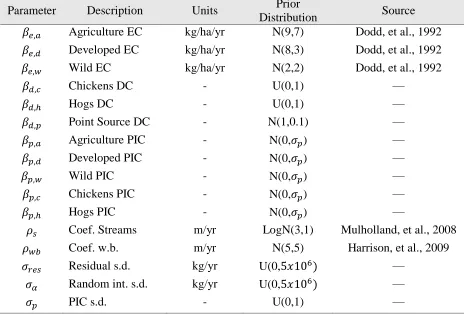
Prior Distributions
Table 1. Model parameters with their prior distributions (or hierarchical distributions in the case of PIC parameters).
Parameter Description Units Prior
Distribution Source 𝛽𝑒,𝑎 Agriculture EC kg/ha/yr N(9,7) Dodd, et al., 1992 𝛽𝑒,𝑑 Developed EC kg/ha/yr N(8,3) Dodd, et al., 1992
𝛽𝑒,𝑤 Wild EC kg/ha/yr N(2,2) Dodd, et al., 1992
𝛽𝑑,𝑐 Chickens DC - U(0,1) —
𝛽𝑑,ℎ Hogs DC - U(0,1) —
𝛽𝑑,𝑝 Point Source DC - N(1,0.1) —
𝛽𝑝,𝑎 Agriculture PIC - N(0,𝜎𝑝) —
𝛽𝑝,𝑑 Developed PIC - N(0,𝜎𝑝) —
𝛽𝑝,𝑤 Wild PIC - N(0,𝜎𝑝) —
𝛽𝑝,𝑐 Chickens PIC - N(0,𝜎𝑝) —
𝛽𝑝,ℎ Hogs PIC - N(0,𝜎𝑝) —
𝜌𝑠 Coef. Streams m/yr LogN(3,1) Mulholland, et al., 2008
𝜌𝑤𝑏 Coef. w.b. m/yr N(5,5) Harrison, et al., 2009
𝜎𝑟𝑒𝑠 Residual s.d. kg/yr U(0,5𝑥106) —
𝜎𝛼 Random int. s.d. kg/yr U(0,5𝑥106) —
𝜎𝑝 PIC s.d. - U(0,1) —
Model parameters were estimated using Hamiltonian (Markov Chain) Monte Carlo (HMC) sampling with the Rstan software operated in R (R. Core Team, 2013; Stan Development Team, 2016). Three parallel sampling chains were run 20,000 iterations each with the first 10,000 discarded as the burn-in period, resulting in 30,000 posterior samples total. Convergence was considered achieved when the scale reduction statistic 𝑅̂—the square
Performance Assessment
Model performance was determined by the Nash-Sutcliffe Efficiency (NSE) (Nash & Sutcliffe, 1970) and mean absolute error (MAE). NSE, which is commonly used in hydrologic modeling, is equivalent to the coefficient of determination as it is often defined in statistic texts (e.g., Faraway, 2016), but different from the square of the Pearson’s correlation coefficient. NSE and MAE were calculated based on the means of the Bayesian posterior predictive distributions. For comparison, these performance metrics were calculated in two different ways – assuming the incremental watershed-specific random effects are known, and assuming they
are unknown (set to zero).
The performance of the full model (calibrated to all data) is compared to a null-source model, and is further evaluated through a 3-fold cross-validation (Elsner & Schmertmann, 1994) where each of the three river basins are treated as a fold. The null-source model is a linear regression where watershed area and precipitation multiplied by watershed area were used as predictor variables of incremental loads within watersheds. The null-source model serves as a benchmark to gage the extent to which representation of specific source types (i.e., land uses, point sources, and CAFO sources) and their spatiotemporal variability improves model performance. For cross-validation, the data were divided into three sections (i.e., folds) by river-basin, where the model is trained by two and tested by one of the three segments, considering all three possible combinations in turn. The cross-validation serves to test the model’s predictive skill, demonstrated by the NSE and MAE, and by comparing parameter
RESULTS
Annual TN Loads
Figure 3. WRTDS estimates of TN loadings at downstream locations on the CFRB, NRB, and TPRB (Kelly, Ft. Barnwell, and Washington, respectively). Points represent annual loading estimates and lines are flow-normalized loads. Vertical lines mark the beginning and
end of the time-series used in the watershed model (1994-2012).
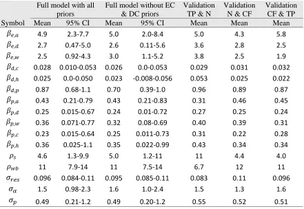
Model Parameterization and Performance
Table 2. Mean parameter estimates with 95% credible intervals for models with and without informative priors on EC and DC. Mean parameter estimates are also shown for each fold of
the cross validation. Parameter units are provided in Table 1.
Symbol
Full model with all priors
Full model without EC & DC priors
Validation TP & N
Validation N & CF
Validation CF & TP
Mean 95% CI Mean 95% CI Mean Mean Mean
𝛽𝑒,𝑎 4.9 2.3-7.7 5.0 2.0-8.4 5.0 4.3 5.8
𝛽𝑒,𝑑 2.7 0.47-5.0 2.6 0.11-5.6 3.6 2.8 2.5
𝛽𝑒,𝑤 2.5 0.92-4.3 3.0 1.1-5.2 3.8 2.5 1.9
𝛽𝑑,𝑐 0.028 0.010-0.053 0.026 0.0-0.053 0.029 0.031 0.032
𝛽𝑑,ℎ 0.025 0.0-0.050 0.023 -0.008-0.056 0.053 0.025 0.022
𝛽𝑑,𝑝 0.87 0.68-1.1 0.70 0.39-1.0 0.96 0.89 0.87
𝛽𝑝,𝑎 0.43 0.21-0.79 0.43 0.21-0.83 0.31 0.46 0.45
𝛽𝑝,𝑑 0.25 0.015-0.67 0.24 0.01-0.72 0.27 0.25 0.24
𝛽𝑝,𝑤 0.36 0.071-0.77 0.32 0.08-0.69 0.40 0.39 0.31
𝛽𝑝,𝑐 0.23 0.015-0.64 0.25 0.011-0.73 0.31 0.22 0.28
𝛽𝑝,ℎ 0.36 0.025-1.1 0.35 0.022-0.99 0.43 0.34 0.34
𝜌𝑠 4.6 1.3-9.9 5.0 1.2-11 11 4.4 4.0
𝜌𝑤𝑏 11 7.9-14 11 7.5-14 6.7 12 11
𝜎𝑟𝑒𝑠 0.096 0.084-0.11 0.095 0.085-0.11 0.083 0.11 0.096
𝜎𝛼 1.5 0.98-2.3 1.6 1.0-2.4 1.5 1.3 1.6
Figure 4. Marginal posterior distributions of model parameters with prior distributions (dashed lines), as determined for the full model. Parameter units are provided in Table 1. `
Hydraulic retention times for both Jordan Lake and Falls Lake are relatively long, potentially causing a lag in downstream station monitoring for upstream TN loadings that exceeds the annual time-step. Mean residence times from 1984 to 2017, calculated by dividing mean outflow by reservoir volume (USACE, 2017), for Jordan Lake and Falls Lake are 0.52 and 0.78 years respectively, with standard deviations of 0.60 and 0.35 years respectively. Both Lillington and Falls Dam watersheds, containing Jordan Lake and Falls Lake, have NSEs of -0.48 and 0.33 respectively, indicating that the large retention times in these watersheds may be contributing to poor estimations of incremental loadings. Still, these watersheds were included in the model since their mean residence times were less than a year, and for the sake of maintaining continuity of TN transport within the river basins.
The model was also calibrated using non-informative priors for EC and DC parameters, so that the influence of the prior information could be more clearly assessed. In most cases, parameter estimates without priors were similar to parameter estimates with priors (Table 2). A notable exception is the EC for hogs, where the 95% CI intersects zero slightly (though the 90% CI does not). While this “no-prior” model is not preferred because prior information from previous studies is ignored and because negative TN loadings are mechanistically impossible, the no-prior model highlights the fact that agricultural and chicken sources are the most strongly identifiable distributed and CAFO source types, respectively, in this study area.
and observed values, the model explains 74% and 68% of variability with random effects included and removed respectively (Appendix L). Temporal autocorrelation in residuals is minimal, with lag-1 correlation coefficients averaging 0.075 across watersheds. In cross validation (without random effects), the model explains 63% of the variability. Mean parameter estimates for all three basin-level folds of the cross validation are similar to each other and to the full model (Table 2), affirming the model is reasonably robust to variations in the training dataset. In comparison, the null-source model explained just 49% of variability using only watershed area and precipitation as predictors.
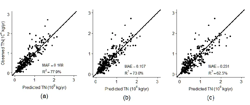
Figure 5. Observed vs. predicted plots of incremental TN loadings using (a) full model with fixed and random effects, (b) full model with fixed effects only, and (c) cross validation with
Nutrient Loading Source Apportionment
Throughout the study period, from 1994 to 2012, TN export estimates reflect a decrease in point-sources, moderate changes in land-use, and a notable increase in CAFOs in many watersheds. Figure 6 shows source-specific TN contributions for of each basin, both before and after accounting for in-stream and water body retention, and using long-term mean precipitation values for each watershed. From 1994 to 2012, point-source discharges of TN decreased by 10% and 61%, in the CFRB and NRB, respectively, and increased by 1.3% in the TPRB. Developed land TN increased by nearly 50% in all three river basins coinciding with a decrease in agriculture land TN of 3.7%, 5.9%, and 3.7% and wild TN of 16%, 29%, and 6.8% in the CFRB, NRB, and TPRB, respectively. Chicken TN export increased by 97% in the CFRB and decreased slightly by 7% and 15% in the NRB and TPRB respectively. Hog TN export increased by 29% and 35% in the CFRB and NRB, respectively, and decreased by 14% in the TPRB. The largest changes in basin-wide percent composition of TN export occurred in the NRB, where in 1994, point, land-use, and CAFO sources made up 26%, 9%, and 65% of basin-wide TN export, respectively; whereas in 2012, the same sources made up 9%, 12%, and 79%, respectively. For the CFRB, livestock sources increased from 12% to 20% and point and land-use sources decreased from 28% to 24% and 60% to 56%, respectively, of the total TN export composition from 1994 to 2012. Percent composition of source contributions changed relatively little for the TPRB.
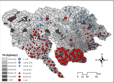
the CFRB, NRB, and TPRB, respectively. TN loading contributions are largest in downstream regions, characterized by higher annual precipitation and lower retention rates (fewer reservoirs), and where most livestock operations and agricultural land is situated (Figure 7). The largest increases in TN loading rates from 1994 to 2012 are in the downstream CFRB because of the growth of chicken and hog operations. Upstream decreases in loading rates are attributable to decreases in point-source loads in the CFRB and NRB and decreases in agriculture land and livestock production in the TPRB. Precipitation has a larger effect on TN loadings in downstream agricultural areas, given that the PIC for agriculture is higher than that of developed and wild land (Appendix I).
Figure 6. TN loading contributions in the CFRB, NRB, and TPRB for (a) 1994 and (b) 2012, by source type. Mean precipitation values are used in calculating loads. Shown are total loadings entering the stream network, including no stream and water body losses (NL),
and loadings at the downstream (DS) basin outlet accounting for stream and water body losses. Downstream locations for each basin are Kelly (CFRB), Ft. Barnwell (NRB), and Washington (TPRM). Chinquapin and Tomahawk watersheds are also included in the CFRB
Figure 7. TN loading rates for the year 2002 (grey shading) and change in loading rate from 1994 to 2012 (points) for each HUC 12. Stream and reservoir retention is included and rates reflect loadings to downstream locations for each basin (Kelly for CFRB, Ft. Barnwell for NRB, and Washington for TPRB). HUC 12 mean precipitation values are used in calculating
loads. TN (kg/ha/yr)
0.0 to 3.0
3.0 to 4.0
4.0 to 5.0
5.0 to 6.0
6.0 to 7.0
7.0 to 8.0
> 8.0
< -1.0
-1.0 to -0.5
-0.5 to -0.1
-0.1 to 0.1
0.1 to 0.5
0.5 to 1.0
> 1.0
.
0 15 30 60DISCUSSION
loading variability. If land use variations are removed, then only 67% of the variability is explained.
While this is perhaps the first study to incorporate temporal changes in both precipitation and source distributions in a nonlinear regression model for watershed loading, similar modeling studies have explored temporal variability using alternative approaches. Wellen et al. (2012) added both interannual climatic variables and dynamic parameter estimation to SPARROW (Smith et al., 1997), thus treating climatic and watershed processes as primary agents of interannual variability. However, unlike our approach, this configuration doesn’t account for land-use change, and precipitation is included as an additive component to
the nonlinear regression rather than as a source-specific modifier of TN export (Wellen et al., 2012). Xia et al (2016) also considered dynamic parameter estimation and land-use change in a nonlinear regression formulation to account for interannual variability in TN export, but did not consider precipitation directly (Xia et al., 2016). Less mechanistic, linear regression models have also been used to study temporal variability in watershed TN loading. For example, Sinha and Michalak (2016) found inter-annual variability in large-scale watershed TN loadings to be driven primarily by both annual precipitation and extreme precipitation events. The effects of precipitation timing and extreme events could also be considered within context of nonlinear regression modeling, perhaps as a future enhancement to the model developed here.
waste TN delivered to streams. Posterior estimates suggest that hog and chicken DCs are very similar and both less than 5% (Figure 4). A 2002 EPA study of CAFO waste management practices across the nation found a mean edge-of-field delivery loss rate of 6% and 9% for hogs and chickens, respectively (Whitman et al., 2002), which are somewhat higher than the DCs determined here. A possible reason for the lower estimates in this study is that some of the livestock contribution may be reflected in the agricultural land EC. To the extent that chicken and hog waste replace other types of fertilizer, these wastes do not constitute an additional load. Furthermore, our DCs do not represent edge-of-field delivery, but rather delivery to the HUC-12 outlet (Figure 7). In any case, our results indicate that chicken and hogs are substantial TN contributors (Figure 6), with mean ECs (calculated by dividing the mean livestock waste delivered to streams by total agriculture land area) of 1.3 and 0.82 kg/ha/yr, respectively. Adding these livestock ECs to the EC for agricultural land (4.9 kg/ha/yr) gives a total effective agricultural EC of 7.0 kg/ha/yr, which is near previous estimates for agricultural land in this region (McMahon et al., 2003; Qian et al., 2005) and the mean literature value (Dodd et al., 1992; Lin, 2004; Harmel et al., 2006).
McMahon et al., 2003; Qian et al., 2005), and may suggest over-reporting of discharger loading rates (Wellen et al., 2012; Schwarz et al., 2006). Developed land EC is on the lower end of literature values for mixed-intensity urban development. Our urban EC estimates are more typical of low-density development (Beaulac & Reckhow, 1982), which comprises the largest portion of developed land-use in the three river basins (Appendix A). The mean EC for point sources (calculated by dividing the mean annual point-source TN delivered to streams by total developed land area) is 5.0 kg/ha/yr, which added to developed land EC gives an effective total developed EC of 7.7 kg/ha/yr, somewhat higher than the effective total agricultural EC (above).
percentile), agriculture land TN export is nearly equal to that of wild land, and developed land export becomes 1.8 times higher than agriculture.
Because not all spatial variation is explained by the deterministic component of this model, watershed random effects account for much of the remaining spatial variability. The random effects term can also indicate spatial correlation among watersheds that might result from regional differences in export rates and watershed processes (e.g. Coastal Plain versus Piedmont). While a previous NC study using data at higher spatial resolution (McMahon et al., 2003; Qian et al., 2005) suggested spatial correlation, the random effects in this study do not exhibit substantial spatial correlation (Appendix J). Systematic differences in nutrient export rates between Piedmont and Coastal Plain watersheds, as suggested in a previous Chesapeake-area study (Jordan et al., 1997), are also not apparent based on the random effects of our study (Appendix I).
from animal waste found in our study. A study by Osburn et al. (2016) found anthropogenic ON in the Neuse to derive mostly from chicken litter, urban street runoff, and eroded sediments either from urban or agricultural sources. Hog waste, however, was found to contribute little ON, though some of this waste could be converted to and be present as soil-derived ON (Osburn et al., 2016). The results of our study generally suggest similar overall contributions from hogs and chickens in the NRB (Figure 6).
Annual effective EC estimates for total agriculture (sum of chicken, hog, and agriculture land ECs) and total urban (sum of point source and developed land ECs) show declining urban and increasing agricultural TN export rates, on average, across the study area (Appendix M). Total urban EC decreased from 10 to 6.4 kg/ha/yr, while total agricultural EC increased from 6.8 to 7.2 kg/ha/yr from 1994 to 2012 during a mean precipitation scenario (Appendix M). The decrease in the total urban export rate results from a decrease in point sources loadings concurrent with an increase in developed area. The increase in TN export rate for total agriculture is attributable to the increase in CAFOs. If CAFOs were not included in the model, the total agricultural EC would remain constant, and there would be no mechanism for exploring the implications of CAFO development within the study region.
under all but the lowest (5th percentile) flow conditions, where agricultural and developed export are approximately equal. This outcome highlights the effectiveness of TMDLs at reducing point sources in the NRB and the remaining challenge of reducing nonpoint sources. Total agricultural TN export increases substantially in the CFRB due mainly to CAFO contributions, while total developed land export increases slightly as a result of increasing urbanization with little reduction in point source loadings (Figure 2, Appendix M).
REFERENCES
Alameddine, I., Qian, S. S., & Reckhow, K. H. (2011). A Bayesian changepoint-threshold model to examine the effect of tmdl implementation on the flow-nitrogen
concentration relationship in the neuse river basin. Water research, 45, 51-62. Alexander, R. B., Böhlke, J. K., Boyer, E. W., David, M. B., Harvey, J. W., Mulholland, P.
J., . . . Wollheim, W. M. (2009). Dynamic modeling of nitrogen losses in river
networks unravels the coupled effects of hydrological and biogeochemical processes. Biogeochemistry, 93, 91-116.
Alexander, R. B., Smith, R. A., & Schwarz, G. E. (2004). Estimates of diffuse phosphorus sources in surface waters of the United States using a spatially referenced watershed model. Water Science and Technology, 49, 1-10.
Altman, J. C., & Paerl, H. W. (2012). Composition of inorganic and organic nutrient sources influences phytoplankton community structure in the New River Estuary, North Carolina. Aquatic Ecology, 46, 269-282.
Beaulac, M. N., & Reckhow, K. H. (1982). An Examination of Land Use-Nutrient Export Relationships. JAWRA Journal of the American Water Resources Association, 18, 1013-1024.
Beck, M. B. (1987). Water quality modeling: a review of the analysis of uncertainty. Water Resources Research, 23, 1393-1442.
Beven, K. (2006). A manifesto for the equifinality thesis. Journal of hydrology, 320, 18-36. Billen, G., Beusen, A., Bouwman, L., & Garnier, J. (2010). Anthropogenic nitrogen
autotrophy and heterotrophy of the worldś watersheds: Past, present, and future trends. Global Biogeochemical Cycles, 24.
Birgand, F., Skaggs, R. W., Chescheir, G. M., & Gilliam, J. W. (2007). Nitrogen removal in streams of agricultural catchments—a literature review. Critical Reviews in
Environmental Science and Technology, 37, 381-487.
Borah, D. K., & Bera, M. (2004). Watershed-scale hydrologic and nonpoint-source pollution models: Review of applications. Transactions of the ASAE, 47, 789.
Burkholder, J. M., Mallin, M. A., Glasgow, H. B., Larsen, L. M., McIver, M. R., Shank, G. C., . . . others. (1997). Impacts to a coastal river and estuary from rupture of a large swine waste holding lagoon. Journal of Environmental Quality, 26, 1451-1466. Burkholder, J., Libra, B., Weyer, P., Heathcote, S., Kolpin, D., Thome, P. S., & Wichman,
M. (2007). Impacts of waste from concentrated animal feeding operations on water quality. Environmental health perspectives, 308-312.
Cahoon, L. B., Mikucki, J. A., & Mallin, M. A. (1999). Nitrogen and phosphorus imports to the Cape Fear and Neuse River basins to support intensive livestock production. Environmental science \& technology, 33, 410-415.
Cambardella, C. A., Moorman, T. B., Jaynes, D. B., Hatfield, J. L., Parkin, T. B., Simpkins, W. W., & Karlen, D. L. (1999). Water quality in Walnut Creek watershed: Nitrate-nitrogen in soils, subsurface drainage water, and shallow groundwater. Journal of Environmental Quality, 28, 25-34.
Cao, W., Bowden, W. B., Davie, T., & Fenemor, A. (2006). Multi-variable and multi-site calibration and validation of SWAT in a large mountainous catchment with high spatial variability. Hydrological Processes, 20, 1057-1073.
Clean Water Act, 33 U.S.C. §1251 et seq (1972).
Conley, D. J., Paerl, H. W., Howarth, R. W., Boesch, D. F., Seitzinger, S. P., Karl, E., . . . Gene, E. (2009). Controlling eutrophication: nitrogen and phosphorus. Science, 123, 1014-1015.
DEQ, N. (2015). A Comparison of PAN and P2O5 Produced from Poultry, Swine and Cattle Operations in North Carolina. North Carolina Department of Environmental Quality.
Dodd, R. C., Cunningham, P. A., Curry, R. J., Liddle, S. K., McMahon, G., Stichter, S., & Tippett, J. P. (1992). Watershed planning in the Albemarle-Pamlico estuarine system. Albemarle-Pamlico Estuarine Study, NC Dept. of Environment, Health, and Natural Resources.
Dodd, R. C., Cunningham, P. A., Curry, R. J., Liddle, S. K., McMahon, G., Stichter, S., & Tippett, J. P. (1992). Watershed planning in the Albemarle-Pamlico estuarine system. Albemarle-Pamlico Estuarine Study, NC Dept. of Environment, Health, and Natural Resources.
Elsner, J. B., & Schmertmann, C. P. (1994). Assessing forecast skill through cross validation. Weather and Forecasting, 9, 619-624.
ESRI . (2011). ArcGIS Desktop: Release 10. Redlands, CA: Environmental Systems Research Institute.
Evans, R. O., Westerman, P. W., & Overcash, M. R. (1984). Subsurface drainage water quality from land application of swine lagoon effluent. Trans. ASAE, 27, 473-480. Falcone, J. A. (2015). US conterminous wall-to-wall anthropogenic land use trends
(NWALT), 1974--2012. Tech. rep., US Geological Survey.
Faraway, J. J. (2016). Extending the linear model with R: generalized linear, mixed effects and nonparametric regression models (Vol. 124). CRC press.
Faulkner, S. (2004). Urbanization impacts on the structure and function of forested wetlands. Urban Ecosystems, 7, 89-106.
Fraterrigo, J. M., & Downing, J. A. (2008). The influence of land use on lake nutrients varies with watershed transport capacity. Ecosystems, 11, 1021-1034.
Garrett, R. G. (1990). Water-quality characteristics of inflow to and outflow from Falls Lake, North Carolina, 1982-87. Department of the Interior, US Geological Survey.
Gelman, A., & Rubin, D. B. (1992). Inference from iterative simulation using multiple sequences. Statistical science, 457-472.
Gelman, A., Carlin, J. B., Stern, H. S., Dunson, D. B., Vehtari, A., & Rubin, D. B. (2014). Bayesian data analysis (Vol. 2). CRC press Boca Raton, FL.
Gilmore, T., Genereux, D., Solomon, D., Farrell, K., & Mitasova, H. (2016). Quantifying an aquifer nitrate budget and future nitrate discharge using field data from streambeds and well nests. (Vol. 52(11)). Water Resources Research.
Gronewold, A. D., & Borsuk, M. E. (2010). Improving water quality assessments through a hierarchical Bayesian analysis of variability. Environmental science \& technology, 44, 7858-7864.
Haith, D. A., & Shoemaker, L. L. (1987). Generalized watershed loading functions for stream flow nutrients. JAWRA Journal of the American Water Resources Association, 23(3), 471-478.
Harden, S. L., & Spruill, T. B. (2008). Factors affecting nitrate delivery to streams from shallow ground water in the North Carolina Coastal Plain. Tech. rep., Geological Survey (US).
Harmel, D., Potter, S., Casebolt, P., Reckhow, K., Green, C., & Haney, R. (2006).
Compilation of measured nutrient load data for agricultural land uses in the United States. JAWRA Journal of the American Water Resources Association, 42, 1163-1178.
Harrison, J. A., Maranger, R. J., Alexander, R. B., Giblin, A. E., Jacinthe, P.-A., Mayorga, E., . . . Wollheim, W. M. (2009). The regional and global significance of nitrogen removal in lakes and reservoirs. Biogeochemistry, 93, 143-157.
Hirsch, R. M., & Cicco, D. a. (2015). User guide to Exploration and Graphics for RivEr Trends (EGRET) and dataRetrieval: R packages for hydrologic data. Tech. rep., US Geological Survey.
Hirsch, R. M., Moyer, D. L., & Archfield, S. A. (2010). Weighted Regressions on Time, Discharge, and Season (WRTDS), with an Application to Chesapeake Bay River Inputs1. JAWRA Journal of the American Water Resources Association, 46, 857-880. Hogan, D. M., & Walbridge, M. R. (2007). Urbanization and nutrient retention in freshwater
riparian wetlands. Ecological Applications, 17, 1142-1155.
Hopkinson, C. S., & Vallino, J. J. (1995). The relationships among man’s activities in watersheds and estuaries: a model of runoff effects on patterns of estuarine community metabolism. Estuaries and Coasts, 18, 598-621.
Howarth, R. W., Billen, G., Swaney, D., Townsend, A., Jaworski, N., Lajtha, K., . . . others. (1996). Regional nitrogen budgets and riverine N & P fluxes for the drainages to the North Atlantic Ocean: Natural and human influences. In Nitrogen cycling in the North Atlantic Ocean and its watersheds (pp. 75-139). Springer.
Johnes, P. J. (1996). Evaluation and management of the impact of land use change on the nitrogen and phosphorus load delivered to surface waters: the export coefficient modelling approach. Journal of hydrology, 183, 323-349.
Jordan, T. E., Correll, D. L., & Weller, D. E. (1997). Nonpoint source discharges of nutrients from Piedmont watersheds of Chesapeake Bay. JAWRA Journal of the American Water Resources Association, 33, 631-645.
Kellogg, R. L., Lander, C. H., Moffitt, D. C., & Gollehon, N. (2000). Manure nutrients relative to the capacity of cropland and pastureland to assimilate nutrients. US
Department of Agriculture, Natural Resources Conservation Service and Agricultural Research Service.
Kelly, C. A., Rudd, J. W., Hesslein, R. H., Schindler, D. W., Dillon, P. J., Driscoll, C. T., . . . Hecky, R. E. (1987). Prediction of biological acid neutralization in acid-sensitive lakes. Biogeochemistry, 3, 129-140.
Kottegoda, N. T., & Rosso, R. (2008). Applied statistics for civil and environmental engineers. Blackwell Malden, MA.
Lebo, M. E., Paerl, H. W., & Peierls, B. L. (2012). Evaluation of progress in achieving TMDL mandated nitrogen reductions in the Neuse River Basin, North Carolina. Environmental management, 49, 253-266.
Lee, S. Y., Dunn, R. J., Young, R. A., Connolly, R. M., Dale, P. E., Dehayr, R., . . . others. (2006). Impact of urbanization on coastal wetland structure and function. Austral Ecology, 31, 149-163.
Lin, J. P. (2004). Review of published export coefficient and event mean concentration
(EMC) data. Tech. rep., ENGINEER RESEARCH AND DEVELOPMENT CENTER VICKSBURG MS.
Lunetta, R. S., Greene, R. G., & Lyon, J. G. (2005). Modeling the distribution of diffuse nitrogen sources and sinks in the Neuse River Basin of North Carolina, USA. JAWRA Journal of the American Water Resources Association, 41, 1129-1147.
Mallin, M. A., & Cahoon, L. B. (2003). Industrialized animal production—a major source of nutrient and microbial pollution to aquatic ecosystems. Population \& Environment, 24, 369-385.
Mallin, M. A., McIver, M. R., Robuck, A. R., & Dickens, A. K. (2015). Industrial swine and poultry production causes chronic nutrient and fecal microbial stream pollution. Water, Air, \& Soil Pollution, 226, 407.
Mattson, M. D., & Isaac, R. A. (1999). Calibration of phosphorus export coefficients for total maximum daily loads of Massachusetts lakes. Lake and Reservoir Management, 15, 209-219.
McMahon, G., Alexander, R. B., & Qian, S. (2003). Support of total maximum daily load programs using spatially referenced regression models. Journal of Water Resources Planning and Management, 129, 315-329.
Mulholland, P. J., Helton, A. M., Poole, G. C., Hall, R. O., Hamilton, S. K., Peterson, B. J., . . . others. (2008). Stream denitrification across biomes and its response to
anthropogenic nitrate loading. Nature, 452, 202-205. N.C. Gen. Stat. (1973). § 143-215.10B.
Nash, J. E., & Sutcliffe, J. V. (1970). River flow forecasting through conceptual models part I—A discussion of principles. Journal of hydrology, 10, 282-290.
NASS, U. (2014). United States Department of Agriculture, National Agricultural Statistics Service. 2012 Census of Agriculture. Retrieved from https://www.agcensus.usda.gov/
National Water Quality Monitoring Council. (2010). Water Quality Portal. Retrieved 10 1, 2016, from https://www.waterqualitydata.us/
National Water Quality Monitoring Council. (n.d.). Water Quality Portal. Retrieved 2016, from https://www.waterqualitydata.us/
NC State University. (2016). 2017 North Carolina Agricultural Chemicals Manual. University of North Carolina PR.
NCDENR. (1994). Tar-Pamlico River Basinwide Water Quality Management Plan. North Carolina Divison of Environmental Management.
NCDENR. (1999). Total maximum daily load for total nitrogen to the Neuse River Estuary, North Carolina. North Carolina Dept. of Environment and Natural Resources, Raleigh, N.C.
NCDENR. (2005). Cape Fear River Basinwide Water Quality Plan. NC Department of Environment & Natural Resources, Raleigh N.C.
NCDENR. (2009). Neuse River Basinwide Water Quality Plan. North Carolina Department of Environemtn and Natural Resources, Raleigh, N.C.
NCDENR. (2014). Swine Waste Management System General Permit. North Carolina Department of Environemtn and Natural Resources, Raleigh, N.C.
NCDEQ. (2017). North Carolina Department of Environmental Quality. Retrieved from 303(d) Files:
https://deq.nc.gov/about/divisions/water-resources/planning/classification-standards/303d/303d-files
Norvell, W. A., Frink, C. R., & Hill, D. E. (1979). Phosphorus in Connecticut lakes predicted by land use. Proceedings of the National Academy of Sciences, 76, 5426-5429.
Osburn, C. L., Handsel, L. T., Peierls, B. L., & Paerl, H. W. (2016). Predicting sources of dissolved organic nitrogen to an estuary from an agro-urban coastal watershed. Environmental Science \& Technology, 50, 8473-8484.
Paerl, H. W., Pinckney, J. L., Fear, J. M., & Peierls, B. L. (1998). Ecosystem responses to internal and watershed organic matter loading: consequences for hypoxia in the eutrophying Neuse River Estuary, North Carolina, USA. Marine Ecology Progress Series, 166, 17.
Paerl, H. W., Scott, J. T., McCarthy, M. J., Newell, S. E., Gardner, W. S., Havens, K. E., . . . Wurtsbaugh, W. A. (2016). It Takes Two to Tango: When and Where Dual Nutrient (N & P) Reductions Are Needed to Protect Lakes and Downstream Ecosystems. Environmental Science \& Technology, 50, 10805-10813.
Qian, S. S., Cuffney, T. F., Alameddine, I., McMahon, G., & Reckhow, K. H. (2010). On the application of multilevel modeling in environmental and ecological studies. Ecology, 91, 355-361.
Qian, S. S., Reckhow, K. H., Zhai, J., & McMahon, G. (2005). Nonlinear regression modeling of nutrient loads in streams: A Bayesian approach. Water Resources Research, 41.
R. Core Team. (2013). R: A Language and Environment for Statistical Computing. Vienna. Retrieved from https://www.r-project.org/
Reavie, E. D., & Baratono, N. G. (2007). Multi-core investigation of a lotic bay of Lake of the Woods (Minnesota, USA) impacted by cultural development. Journal of Paleolimnology, 38, 137-156.
Reckhow, K. H. (2003). On the need for uncertainty assessment in TMDL modeling and implementation. Journal of Water Resources Planning and Management, 129, 245-246.
Reckhow, K. H., & Chapra, S. C. (1999). Modeling excessive nutrient loading in the environment. Environmental Pollution, 100, 197-207.
Rode, M., Arhonditsis, G., Balin, D., Kebede, T., Krysanova, V., Van Griensven, A., & der Zee, V. a. (2010). New challenges in integrated water quality modelling.
Hydrological Processes, 24, 3447-3461.
Rothenberger, M. B., Burkholder, J. M., & Brownie, C. (2009). Long-term effects of changing land use practices on surface water quality in a coastal river and lagoonal estuary. Environmental Management, 44, 505-523.
S.L. 1997-458. (1997). Moratoria on Construction and Expansion of Swine Farms. Schwarz, G. E., Hoos, A. B., Alexander, R. B., & Smith, R. A. (2006). The SPARROW
surface water-quality model: theory, application and user documentation. US geological survey techniques and methods report, book, 6, 248.
Shrestha, S., Kazama, F., & Newham, L. T. (2008). A framework for estimating pollutant export coefficients from long-term in-stream water quality monitoring data. Environmental Modelling \& Software, 23, 182-194.
Sinha, E., & Michalak, A. M. (2016). Precipitation Dominates Interannual Variability of Riverine Nitrogen Loading across the Continental United States. Environmental science \& technology, 50, 12874-12884.
Smith, R. A., Schwarz, G. E., & Alexander, R. B. (1997). Regional interpretation of water-quality monitoring data. Water resources research, 33, 2781-2798.
Smith, R. A., Schwarz, G. E., & Alexander, R. B. (1997). Regional interpretation of water-quality monitoring data. Water resources research, 33, 2781-2798.
Spruill, T. B., Tesoriero, A. J., Mew, H. E., Farrell, K. M., Harden, S. L., Colosimo, A. B., & Kraemer, S. R. (2005). Geochemistry and characteristics of nitrogen transport at a confined animal feeding operation in a coastal plain agricultural watershed, and implications for nutrient loading in the Neuse River Basin, North Carolina, 1999-2002. Tech. rep., U. S. Geological Survey.
Stan Development Team. (2016). RStan: the R interface to Stan. Retrieved from http://mc-stan.org/
State Climate Office of North Carolina. (2016). Climate Retrieval and Observations Network Of the Southeast (CRONOS). Retrieved from http://climate.ncsu.edu/cronos
U.S. Census Bureau. (2017, September 1). Maps and Data. Retrieved from https://www.census.gov/geo/maps-data/
US Army Corps of Engineers. (2017, October 29). Water Management. Retrieved from http://epec.saw.usace.army.mil/
US EPA. (2015). Basins 4.1 (Better Assessment Science Integrating point & Non-point Sources) Modeling Framework. RTP, North Carolina: National Exposure Research Laboratory. Retrieved April 2017, from https://www.epa.gov/exposure-assessment-models/basins
US Geological Survey. (2009). The National Map. Retrieved 4 1, 2017, from https://nationalmap.gov/index.html
USDA-NASS. (2016). US Department of Agriculture National Agricultural Statistics Service. Retrieved from https://www.nass.usda.gov/
USEPA. (2000). Profile of the Agricultural Livestock Production Industry. Retrieved from https://www.nrcs.usda.gov/Internet/FSE_DOCUMENTS/stelprdb1044373.pdf USGS. U.S. Geological Survey. (2017). National Elevation Dataset. Retrieved from
https://nationalmap.gov/elevation.html
Vollenweider, R. A., & others. (1971). Scientific fundamentals of the eutrophication of lakes and flowing waters, with particular reference to nitrogen and phosphorus as factors in eutrophication. Organisation for economic co-operation and development Paris.
Wellen, C., Arhonditsis, G. B., Labencki, T., & Boyd, D. (2012). A Bayesian methodological framework for accommodating interannual variability of nutrient loading with the SPARROW model. Water Resources Research, 48.
Whitman, C. T., Frace, S. E., Mehan, T., Shriner, P. H., & Wrenn, B. (2002). Pollutant Loading Reductions for the Revised Effluent Limitations Guidelines for Concentrated Animal Feeding Operations.
Xia, Y., Weller, D. E., Williams, M. N., Jordan, T. E., & Yan, X. (2016). Using Bayesian hierarchical models to better understand nitrate sources and sinks in agricultural watersheds. Water research, 105, 527-539.
Appendix A. NWALT Land-Use Classifications
NWALT land-use classifications with their respective areas (ha) and % of total area
in all three river basins (Falcone, 2015).
Area (hectares) % of total area Land Use Classification 1992 2002 2012 1992 2002 2012
Water
Water 21548 21548 21960 1.2 1.2 1.2
Wetlands 130783 130783 130783 7.3 7.3 7.3
Developed
Major Transportation 26197 28453 30156 1.5 1.6 1.7 Commercial/Services 30030 35111 38592 1.7 2.0 2.2 Industrial/Military 10842 12392 13884 0.6 0.7 0.8
Recreation 6997 8049 8669 0.4 0.5 0.5
Residential, High Density 14185 20450 26935 0.8 1.1 1.5 Residential, Low-Medium
Density 64792 75844 90279 3.6 4.3 5.1
Developed, Other 22929 17494 12631 1.3 1.0 0.7 Semi-Developed
Urban Interface High 25584 23495 21489 1.4 1.3 1.2 Urban Interface Low Medium 129582 217673 267704 7.3 12.2 15.0
Anthropogenic Other 599 531 448 0.0 0.0 0.0
Production
Mining/Extraction 1031 1060 1136 0.1 0.1 0.1
Crops 335551 318468 318840 18.9 17.9 17.9
Pasture/Hay 165608 165823 156385 9.3 9.3 8.8
Grazing Potential 8403 8258 8363 0.5 0.5 0.5
Low Use
Low Use 784342 693572 630749 44.1 39.0 35.4
Very Low Use, Conservation
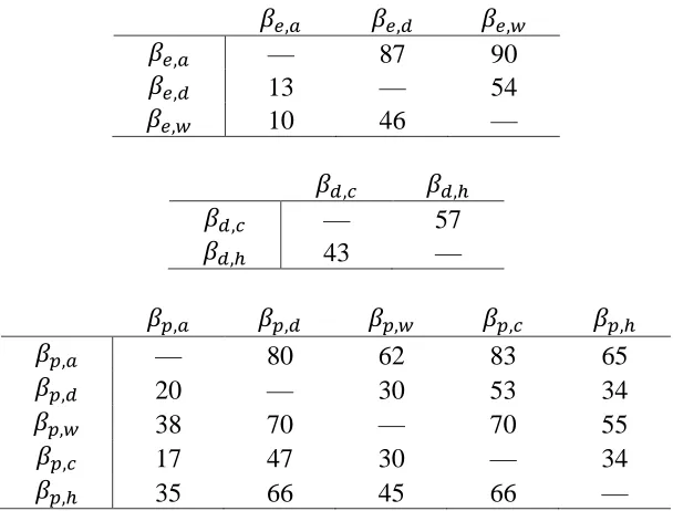
Appendix B. Probabilistic Comparison of Parameter Magnitudes
Table values represent the percent probability of row parameter exceeding column parameter.
𝛽𝑒,𝑎 𝛽𝑒,𝑑 𝛽𝑒,𝑤
𝛽𝑒,𝑎 — 87 90
𝛽𝑒,𝑑 13 — 54
𝛽𝑒,𝑤 10 46 —
𝛽𝑑,𝑐 𝛽𝑑,ℎ
𝛽𝑑,𝑐 — 57
𝛽𝑑,ℎ 43 —
𝛽𝑝,𝑎 𝛽𝑝,𝑑 𝛽𝑝,𝑤 𝛽𝑝,𝑐 𝛽𝑝,ℎ
𝛽𝑝,𝑎 — 80 62 83 65
𝛽𝑝,𝑑 20 — 30 53 34
𝛽𝑝,𝑤 38 70 — 70 55
𝛽𝑝,𝑐 17 47 30 — 34
Appendix C. Modified Export Coefficients Including the PIC for Each Source
The table below lists the modified export coefficients, including the PIC for each source type (kg/ha/yr). Included are TN export for mean precipitation (prec. = 0) and positive and negative standard deviation of precipitation ranges (prec. = −+1) and the 95 percentile of precipitation ranges (prec. = −+1. 96).
Source prec. = 0 𝑝𝑟𝑒𝑐. = 1−+ 𝑝𝑟𝑒𝑐. = 1−+ . 96 Agriculture
4.9 2.8-7.0 0.77-9.0
Developed
2.7 2.0-3.4 1.4-4.0
Wild
2.5 1.6-3.4 0.74-4.3
Chicken
0.028 0.022-0.034 0.015-0.041 Hog
Appendix D. Coefficient of Variation (CV) Values from the WRTDS Uncertainty Analysis
The figure below shows the Coefficient of Variation (CV) values for the 8 sampling schedules used in the WRTDS uncertainty analysis by station location. The dashed line is the fit power regression used in this study.
0 0.1 0.2 0.3 0.4 0.5 0.6
0 50 100 150 200 250 300
CV
Samples days per year
Appendix E. Mean Annual TN Loads from Point Source Dischargers from 1994 to 2012
Appendix F. Land Use Change Maps
The figures below show land use change for 1992 (a) and 2012 (b). Land use types included are agriculture (yellow), developed (red), wild (green), and water/wetlands (blue). Black outlines are the watersheds used in this study.
Appendix G. WRTDS TN Estimates for Stations in Each River Basin
The figures below show WRTDS TN estimates for stations in the NRB (a), CFRB (b), and TPRB (c) from 1994 to 2015. Points are annual estimates and lines are
flow-normalized estimates. Stations for the NRB include Falls Dam (FD), Clayton (C), Goldsboro (G), Kinston (K), and Ft. Barnwell (FB). Stations for the CFRB include Kelly (K), Tarheel (Tar), Lillington (Lil), Moncure (M), Bynum (By), Burlington (B), Tomahawk (Tom),
Chinquapin (C), and Ramseur (R). Stations for the TPRB include Washington (W), Tarrboro (T), Rocky Mount (RM), Louisburg (L), and I96 (I).
(b)
Appendix H. Percent TN Retention Map
The map below shows percent TN retention from each HUC12 to downstream points for each basin (Kelly for all CFRB watersheds except Chinquapin and Tomahawk, Ft. Barnwell for NRB, and Washington for TPRB). Black outlines are the watersheds used in this study.
% TN Retention
0 to 10
10 to 20
20 to 30
30 to 40
40 to 50
50 to 60
> 60
0 15 30 60 Km
Appendix I. TN Loading Rate Maps
The maps below show TN loading rates (kg/ha/yr) using 5th (a) and 95th (b) percentile precipitation values for each HUC 12. Also shown are TN loading rates not including stream and water body retention using mean precipitation values (c) for each HUC 12. Loading rates for the year 2002 are in grey shading and points reflect change in rates from the year 1994 to 2012. In maps (a) and (b) stream and reservoir retention is included and rates reflect loadings to downstream locations for each basin (Kelly for CFRB, Ft. Barnwell for NRB, and Washington for TPRB).
(a)
TN kg/ha/yr
0.0 to 3.0
3.0 to 4.0
4.0 to 5.0
5.0 to 6.0
6.0 to 7.0
7.0 to 8.0
> 8.0
< -1.0
-1.0 to -0.5
-0.5 to -0.1
-0.1 to 0.1
0.1 to 0.5
0.5 to 1.0
> 1.0
0 15 30 60 Km
(b)
TN kg/ha/yr
0.0 to 3.0
3.0 to 4.0
4.0 to 5.0
5.0 to 6.0
6.0 to 7.0
7.0 to 8.0
> 8.0
< -1.0
-1.0 to -0.5
-0.5 to -0.1
-0.1 to 0.1
0.1 to 0.5
0.5 to 1.0
> 1.0
0 15 30 60 Km
(c)
TN kg/ha/yr
0.0 to 3.0
3.0 to 4.0
4.0 to 5.0
5.0 to 6.0
6.0 to 7.0
7.0 to 8.0
> 8.0
< -1.0
-1.0 to -0.5
-0.5 to -0.1
-0.1 to 0.1
0.1 to 0.5
0.5 to 1.0
> 1.0
0 15 30 60 Km
Appendix J. Values of Random Intercept Term α by Watershed
TN
100,000 kg/ha/yr
< -2.0
-2.0 to -1.0
-1.0 to 0.0
0.0 to 1.0
1.0 to 2.0
> 2.0
.
Appendix L. Log Observed vs. Predicted Plots of Incremental TN
Appendix M. Effective Export Rates and Loadings
Effective export rates (kg/ha/yr) for all three basins (i) and effective loadings (kg/yr) for the TPRB (ii), NRB (iii), and CFRB (iv), are shown in the figures below. Developed (solid) and agriculture (dashed) effective loadings or export rates are calculated using the mean (a), 5th (b) and 95th (c) percentile precipitation values.
(ii)