Volume 2008, Article ID 647135,7pages doi:10.1155/2008/647135
Research Article
A Fault Diagnosis Approach for Gears Based on
IMF AR Model and SVM
Junsheng Cheng, Dejie Yu, and Yu Yang
The State Key Laboratory of Advanced Design and Manufacturing for Vehicle Body, Hunan University, Changsha 410082, China
Correspondence should be addressed to Junsheng Cheng,signalp@tom.com
Received 24 July 2007; Revised 28 February 2008; Accepted 15 April 2008
Recommended by Nii Attoh-Okine
An accurate autoregressive (AR) model can reflect the characteristics of a dynamic system based on which the fault feature of gear vibration signal can be extracted without constructing mathematical model and studying the fault mechanism of gear vibration system, which are experienced by the time-frequency analysis methods. However, AR model can only be applied to stationary signals, while the gear fault vibration signals usually present nonstationary characteristics. Therefore, empirical mode decomposition (EMD), which can decompose the vibration signal into a finite number of intrinsic mode functions (IMFs), is introduced into feature extraction of gear vibration signals as a preprocessor before AR models are generated. On the other hand, by targeting the difficulties of obtaining sufficient fault samples in practice, support vector machine (SVM) is introduced into gear fault pattern recognition. In the proposed method in this paper, firstly, vibration signals are decomposed into a finite number of intrinsic mode functions, then the AR model of each IMF component is established; finally, the corresponding autoregressive parameters and the variance of remnant are regarded as the fault characteristic vectors and used as input parameters of SVM classifier to classify the working condition of gears. The experimental analysis results show that the proposed approach, in which IMF AR model and SVM are combined, can identify working condition of gears with a success rate of 100% even in the case of smaller number of samples.
Copyright © 2008 Junsheng Cheng et al. This is an open access article distributed under the Creative Commons Attribution License, which permits unrestricted use, distribution, and reproduction in any medium, provided the original work is properly cited.
1. INTRODUCTION
The process of gear fault diagnosis includes the acquisition of information, extracting feature, and recognizing conditions, in which the last two are the prior.
Signal processing methods have been widely used to
extract fault feature of gear vibration signals [1,2]. Fourier
transform (FT), which has been the dominating analysis tool for feature extraction of stationary signals, could produce the statistical average characteristics over the entire duration of the data. However, it fails to provide the whole and local features of the signal in time and frequency domain. Unfortunately, the gear fault vibration signals exactly present nonstationary characteristics. On the other hand, the time-frequency analysis methods can generate both time and frequency information of a signal simultaneously. Therefore, in the most recent studies, the time-frequency analysis
methods are used in gear fault feature extraction [3–5].
Among all the available time-frequency analysis methods,
the wavelet transform may be the best one [6,7], however,
it still has some inevitable deficiencies [8]. Firstly, energy
leakage will occur when wavelet transform is used to process signals due to the fact that wavelet transform is essentially an adjustable windowed Fourier transform. Secondly, the appropriate base function needs to be selected in advance. Moreover, once the decomposition scales are determined, the results of wavelet transform would be the signal under a certain frequency band. Therefore, wavelet transform is not a self-adaptive signal processing method in nature. In addition, the mathematical model needs to be established or the fault mechanism of the gear vibration system needs to be studied before the feature extraction in
above-mentioned methods, which usually are quite difficult to be
condition; more importantly, an accurate AR model can reflect the characteristics of a dynamic system. Additionally, it is indicated that the autoregression parameters of AR
model are very sensitive to the condition variation [9,10].
The gear fault vibration signals own shock characteristics, whereas AR model can model transients and its frequency response function can be calculated from autoregression parameters of AR model. Therefore, the autoregression parameters can be used to analyze the condition variation of dynamic systems. However, when the AR model is
applied to nonstationary signals, it is difficult to estimate
autoregression parameters by the least square method or Yule-Walker equation method. The time-dependent autore-gressive and moving average (ARMA) model, on the other hand, can be applied to nonstationary signals, but the more computation time is needed. Furthermore, only when the time-dependent ARMA model is applied to the commonly linear frequency and amplitude modulated signals, can the satisfactory results be obtained [11]. Therefore, it is necessary to preprocess the vibration signals before the AR model is generated. Empirical mode decomposition (EMD) is anew time-frequency analysis method proposed by Huang et al.
[12, 13], which is based on the local characteristic time
scale of signal and decomposes the complicated signal into a number of intrinsic mode functions (IMFs). By analyzing each IMF component that involves the local characteristic of the signal, the features of the original signal could
be extracted more accurately and effectively. In addition,
the frequency components involved in each IMF not only relates to sampling frequency but also changes with the signal itself, therefore EMD is a self-adaptive time frequency analysis method that is perfectly applicable to nonlinear and nonstationary processing. Now EMD method has been widely applied to the mechanical fault diagnosis and
con-dition monitoring. In [14], EMD method is combined with
smoothed nonlinear energy operator to detect flute breakage.
The results demonstrate that this method can efficiently
monitor the conditions of the endmill under varying cutting
conditions. In [15], a fault diagnosis method for sheet
metal stamping process based on EMD and learning vector quantization is proposed. The results show that this method could successfully detect the artificially created defects. In this paper, targeting the nonstationary characteristics of gear vibration signal and disadvantage of AR model, a fault feature extraction method in which IMF and AR model are combined is proposed.
After the feature extraction, the pattern recognition is
another point of gears fault diagnosis [16–18]. Conventional
statistical pattern recognition methods and artificial neural networks (ANNs) classifiers are studied based on the premise
that the sufficient samples are available, which is not
always true in practice [19]. In recent years, support vector
machines (SVMs) have been found to be remarkably effective
in many real-world applications [20–23]. They are based
on statistical learning theories that are of specialties for a smaller sample number and have better generalization than ANNs and guarantee that the extremum and global optimal solution are exactly the same. Meantime, SVMs can solve the
learning problem of a smaller number of samples [24,25].
Due to the fact that it is difficult to obtain sufficient fault
samples in practice, SVMs are introduced into gears fault diagnosis due to their high accuracy and good generalization for a smaller sample number in this paper.
2. EMD METHOD
EMD method is developed from the simple assumption that
any signal consists of different simple intrinsic modes of
oscillations. Each linear or nonlinear mode will have the same number of extrema and zero-crossings. There is only one extremum between successive zero-crossings. Each mode should be independent of the others. In this way, each signal could be decomposed into a number of intrinsic mode functions (IMFs), each of which must satisfy the following definition [12,13].
(1) In the whole dataset, the number of extrema and the
number of zero-crossings must either equal or differ
at most by one.
(2) At any point, the mean value of the envelope defined by local maxima and the envelope defined by the local minima is zero.
An IMF represents a simple oscillatory mode compared with the simple harmonic function. With the definition, any
signalx(t) can be decomposed as follows.
(1) Identify all the local extrema, then connect all the local maxima by a cubic spline line as the upper envelope.
(2) Repeat the procedure for the local minima to produce the lower envelope. The upper and lower envelopes should cover all the data between them.
(3) The mean of upper and lower envelope value is
designated asm1, and the difference between the signalx(t)
andm1is the first component,h1:
x(t)−m1=h1. (1)
Ideally, ifh1is an IMF, thenh1is the first IMF component of
x(t).
(4) Ifh1is not an IMF,h1is treated as the original signal and repeat (1), (2), (3), then
h1−m11=h11. (2)
After repeated sifting, that is, up toktimes,h1kbecomes an
IMF:
h1(k−1)−m1k=h1k, (3)
then it is designated as
c1=h1k, (4)
the first IMF component from the original data. (5) Separatec1fromx(t), we could get
r1=x(t)−c1, (5)
r1 is treated as the original data and repeat the above
0 0.1 0.2 0.3 0.4 0.5 0.6 0.7 0.8 0.9 1 Timet(s)
−50 0 50
A
cce
le
ra
ti
o
n
a
(ms
−
2)
Figure 1: Acceleration vibration signal of a gear with a broken
tooth.
could be got. Let us repeat the process as described above for
ntimes, thenn-IMFs of signalx(t) could be got. Then,
r1−c2=r2 .. . rn−1−cn=rn.
(6)
The decomposition process can be stopped when rn
becomes a monotonic function from which no more IMF can
be extracted. By summing up (5) and (6), we finally obtain
x(t)=
n
j=1
cj+rn. (7)
Thus, one can achieve a decomposition of the signal
inton-empirical modes and a residuern, which is the mean
trend ofx(t). Each of the IMFsc1,c2,. . .,cnincludes different
frequency bands ranging from high to low and is stationary.
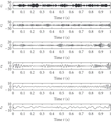
Figure 1shows an acceleration vibration signal of a gear with a broken tooth. It is decomposed into 5 IMFs and a
remnantrnby using EMD method asFigure 2illustrates. It
can be concluded fromFigure 2that each IMF component
implies distinct time characteristic scale.
3. SUPPORT VECTOR MACHINES (SVMs)
SVM is developed from the optimal separation plane under linearly separable condition. Its basic principle can be
illustrated in two-dimensional way asFigure 3[25].Figure 3
shows the classification of a series of points for two different
classes of data, class A (circles) and class B (stars). The SVM
tries to place a linear boundary H between the two classes
and orients it in such way that the margin is maximized, namely, the distance between the boundary and the nearest data point in each class is maximal. The nearest data points are used to define the margin and are known as support vectors.
Suppose there is a given training sample set G =
{(xi,yi), i=1· · ·l}, each samplexi∈Rd belongs to a class
byy∈ {+1,−1}. The boundary can be expressed as follows:
ω·x+b=0, (8)
0 0.1 0.2 0.3 0.4 0.5 0.6 0.7 0.8 0.9 1 Timet(s)
−500 50
c1
0 0.1 0.2 0.3 0.4 0.5 0.6 0.7 0.8 0.9 1 Timet(s)
−500 50
c2
0 0.1 0.2 0.3 0.4 0.5 0.6 0.7 0.8 0.9 1 Timet(s)
−200 20
c3
0 0.1 0.2 0.3 0.4 0.5 0.6 0.7 0.8 0.9 1 Timet(s)
−100 10
c4
0 0.1 0.2 0.3 0.4 0.5 0.6 0.7 0.8 0.9 1 Timet(s)
−100 10
c5
0 0.1 0.2 0.3 0.4 0.5 0.6 0.7 0.8 0.9 1 Timet(s)
−100 10
rn
Figure2: The EMD results of a gear vibration signal.
Support vector Support vector
Support vector Margin
H2
H
H1
Figure3: Classification of data by SVM.
whereωis a weight vector andbis a bias. So the following
decision function can be used to classify any data point in eitherclass A or B:
f(x)=sign(ω·x+b). (9)
The optimal hyperplane separating the data can be obtained as a solution to the following constrained optimiza-tion problem:
minimize 1
2ω
2 ,
subject to yi
ω·xi
Introducing Lagrange multipliersαi ≥ 0, the
optimiza-tion problem can be rewritten as
minimize L(ω,b,α)=
l
i=1 αi−
1 2
l
i,j=1 αiαjyiyj
xi·xj
,
subject to αi≥0,
l
i=1
αiyi=0.
(11)
The decision function can be obtained as follows:
f(x)=sign
l
i=1 αiyi
xi·x
+b
. (12)
If the linear boundary in the input spaces is not enough to separate into two classes properly, it is possible to create a hyperplane that allows linear separation in the higher dimension. In SVM, it is achieved by using a transformation
Φ(x) that maps the data from input space to feature space. If
a kernel function
K(x,y)=Φ(x)·Φ(y) (13)
is introduced to perform the transformation, the basic form of SVM can be obtained:
f(x)=sign
l
i=1 αiyiK
x,xi
+b
. (14)
Among the kernel functions in common use are linear functions, polynomials functions, radial basis functions, and sigmoid functions.
4. DIAGNOSIS APPROACH FOR GEARS BASED ON IMF AR MODEL AND SVM
The following autoregressive model AR(m) could be
estab-lished for each IMF componentci(t) in (7) [26]:
ci(t) + m
k=1
ϕikci(t−k)=ei(t), (15)
where ϕik (k = 1, 2,. . .,m), m are the model parameters
and model order of the autoregressive model AR(m) of
ci(t), respectively; ei(t) is the remnant of the model and
is a white noises sequence whose mean value is zero and
variance is σ2
i. Since the parameters ϕik can reflect the
inherent characteristics of a gear vibration system and the
variance of the remnantσ2
i is tightly related with the output
characteristics of the system, ϕik and σi2 can be chosen as
feature vectors Ai = [ϕi1,ϕi2,. . .,ϕim,σi2] to identify the
condition of the gears system.
The flow chart of a diagnosis method proposed in this paper is illustrated inFigure 4.
The fault diagnosis approach for gearsbased on IMF AR model and SVM is represented as follows.
(1) Sample signalsNtimes at a certain sample frequency
fsunder the circumstance that the gear is normal and the
Start
Input original signalx(t)
IMF componentsc1,c2,. . .,cnare obtained after applying EMD tox(t)
AR model is created for each IMF componentci(t)
Extract feature vectorsAi
SVM classifier
Identify the condition of the gears
End
Figure4: The flow chart of the proposed method.
gear has the crack faults. And the 2N signals are taken
as samples that are divided into two subsets, the training samples and test samples.
(2) Each signal is decomposedby EMD. Different signal
has different amount of the IMFs, denoted byn1,n2,. . .,n2N,
and let n = max(n1,n2,. . .,n2N). If some samples whose
amount nk (k = 1, 2,. . ., 2N) of IMF components is less
than n, it can be padded with zero to n components
c1(t),c2(t),. . .,cn(t), that isci(t) = {0}, i = nk+ 1,nk +
2,. . .,n.
(3) In order to eliminate the effect of the signal amplitude
to the variance of the remnant σi2, normalize each IMF
component to achieve a new component:
ci(t)=∞ci(t)
−∞ci2(t)dt
. (16)
(4) Establish AR model for the normalized component,
determine the order mof the model and estimate
autore-gressive parametersϕik (k = 1, 2,. . .,m) and the remnant’s
varianceσ2
i, whereϕikmeans thekth autoregressive
param-eters of the ith IMF component. Therefore, the feature
vector used as input vector of SVMs is as follows: Ai =
ϕi1,ϕi2,. . .,ϕim,σi2
.
(5) Separate the training set into two classes:y=+1 and
y= −1, which represent two kinds of working condition of
the gears, namely, the normal gear and the gear with crack
fault. Actually, the decision function f(x) is determined
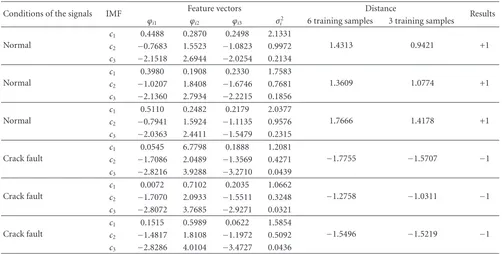
Table1: The identification results based on IMF AR model and SVM.
Conditions of the signals IMF Feature vectors Distance Results
ϕi1 ϕi2 ϕi3 σi2 6 training samples 3 training samples
Normal
c1 0.4488 0.2870 0.2498 2.1331
1.4313 0.9421 +1
c2 −0.7683 1.5523 −1.0823 0.9972
c3 −2.1518 2.6944 −2.0254 0.2134
Normal
c1 0.3980 0.1908 0.2330 1.7583
1.3609 1.0774 +1
c2 −1.0207 1.8408 −1.6746 0.7681
c3 −2.1360 2.7934 −2.2215 0.1856
Normal
c1 0.5110 0.2482 0.2179 2.0377
1.7666 1.4178 +1
c2 −0.7941 1.5924 −1.1135 0.9576
c3 −2.0363 2.4411 −1.5479 0.2315
Crack fault
c1 0.0545 6.7798 0.1888 1.2081
−1.7755 −1.5707 −1
c2 −1.7086 2.0489 −1.3569 0.4271
c3 −2.8216 3.9288 −3.2710 0.0439
Crack fault
c1 0.0072 0.7102 0.2035 1.0662
−1.2758 −1.0311 −1
c2 −1.7070 2.0933 −1.5511 0.3248
c3 −2.8072 3.7685 −2.9271 0.0321
Crack fault
c1 0.1515 0.5989 0.0622 1.5854
−1.5496 −1.5219 −1
c2 −1.4817 1.8108 −1.1972 0.5092
c3 −2.8286 4.0104 −3.4727 0.0436
5. APPLICATIONS
An experiment has been carried out on the small experiment-rig developed by the Vibration and Test Center of Hunan University itself. The fault is introduced by cutting slot with laser in the root of tooth, and the width of the slot is 0.15–0.25 mm, as well as its depth is 0.1–0.3 mm. The acceleration sensor has been fixed on the cover of the gear box before 30 signals under two circumstances are sampled with sample frequency of 1024 Hz, among which three randomly chosen samples for each condition are taken as training samples, and the remain are test data.
Decompose each vibration signals under different
condi-tions with EMD method into a number of IMFs. The analysis results show that the fault information of gear vibration signals is mainly included in the first three IMF components. Therefore, the AR models of the first three IMF components are established merely. In this paper, the order of the model,
m, is determined with FPE criterion [26]; the autoregressive
parametersϕik (k = 1, 2,. . .,m) and the remnant variance
σi2 of the model are computed with least squares criterion
[26]. As, in fact, the system condition is mainly decided by
the autoregressive parameters of the first several ones and the remnant variance, those of only the first three ones, that is ϕik (k=1, 2, 3) andσi2, are chosen as feature vectors in this
paper for convenience.
Define the normal condition asy=+1 and the one with
the crack fault asy= −1; choose the linear kernel function to
calculate and by formulas (11) we can obtain the parameters
of SVM classifier, α = [0, 0.1699, 0.6091, 0.7790, 0, 0]T,
ω = 1.2482, and b = 2.5942. Then, by formula (12)
the identification result of each test sample is obtained, part
of which are shown inTable 1. Obviously, the identification
results are totally consistent with the fact. For further study of the application of SVMs in the pattern identification with smaller number of samples, the number of training samples decrease to three (one is normal and the others is with crack fault) and the calculation procedure is the same as above. Here, the parameters of the SVM classifier become
α = [0.5014, 0.5014, 0]T,ω = 1.0014,b = 2.5485. The
identification results to the same test samples are shown in
Table 1too.
It can be seen from Table 1 that SVM classifier can
still classify the two conditions of gears accurately after the training samples are decreased, which confirm fully that the SVM classifier can be applied successfully to the pattern recognition even in cases where only limited training samples are available. It also can be found, if we compare
the distances between test samples with different number
of training samples to the optimal separating hyperplane
H, that the distance decreases after the number of training
samples become smaller although the gear work states can still be identified by SVM, which shows that in this way the whole performance of the classifier somewhat reduces.
What we discuss above is how to classify two conditions of gears (normal and crack fault), that is, two-class problem. When it comes to the multiple-class problems, that is, how to identify the gears with multiple-class faults (e.g., crack, broken teeth, etc.), generalizing method can be introduced to decompose the multiple-class problems into two-class problems which then can be trained with SVM. In other words, each time take one group of the training samples as one class and therest, which do not belong to the former,
can be taken as the other class. Hence, for the k(k ≥ 3)
classes’ problems, the classification of the input space can be
Table2: The identification results based on IMF AR model and SVMs.
Conditions of the signals SVM classifier Identification results
SVM1 SVM2 SVM3
Normal +1 Normal
Normal +1 Normal
Crack fault −1 +1 Crack fault
Crack fault −1 +1 Crack fault
Broken teeth −1 −1 +1 Broken teeth
Broken teeth −1 −1 +1 Broken teeth
Three SVM classifiers are needed to design if three classes of gear work conditions are to be identified like normal, with crack fault and with broken teeth fault. First of all,
define that y = +1 represents the normal condition and
y = −1 represents the faults condition, that is, identify the
gear whether it has fault or not by SVM1. Secondly, identify the gear whether it has crack fault or not by SVM2, here
y =+1 represents crack fault and y = −1 represents other
faults. Finally, identify the gear whether it has broken teeth
fault or not, here y =+1 represents broken teeth fault and
y= −1 represents other faults. The identification approach
is the same as above, that is, extract nine samples as training ones at random (three samples with normal condition, three samples with crack fault, and three samples with broken teeth fault); and then calculate the parameters of SVM classifier.
The part identification results are shown in Table 2 from
which we can see that three SVM classifiers can identify the working conditions and fault patterns of gears accurately.
6. CONCLUSIONS
AR model is an information container that contains the characteristics of gear vibration systems, based on which the fault feature of gear vibration signal can be extracted. The most important is that the gear work states can be identified by the parameters of the AR model after the AR model of vibration signals is established without constructing mathematical model and studying the fault mechanism. However, AR model can only be applied to stationary signals, while the gear fault vibration signals always display nonstationary behavior. To target this problem, in this paper before AR model is established, a preprocessing on gear fault vibration signals is carried out with EMD method, which can decompose a signal, in terms of its intrinsic information, into a number of IMFs. The decomposition of EMD is a process of origin signal linearization and stationary in nature, thus AR model can be established for each of the IMF components.
The limitations of the conventional statistical pattern recognition methods and ANNs classifies are targeted. Support vector machine, which has better generalization than ANNs and can solve the learning problem of smaller number of samples quite well, has been introduced into the pattern recognition.
By the analysis results of three kinds of gears vibration signals among which one is normal and the other two are the gears with crack and gears with broken tooth faults respectively, it has been shown that the gear fault diagnosis
approach based on IMF AR model and SVM can be applied to classify the gear working conditions and fault patterns
effectively and accurately even in case of smaller number of
samples, which accordingly offers a new approach for the
fault diagnosis of gears. However, because it would take more time to determine the parameters of SVM classifier and the AR model, the proposed method cannot be available in real-time. In addition, what is necessary to point out is that the SVM theory is still in its perfecting phase, for example, the
problems of kernel functions selection in different condition
and so on are still needed to research further.
ACKNOWLEDGMENT
The support for this research under Chinese National Science Foundation Grant no. 50775068 is gratefully acknowledged.
REFERENCES
[1] W. Q. Wang, F. Ismail, and M. F. Golnaraghi, “Assessment of gear damage monitoring techniques using vibration measure-ments,”Mechanical Systems and Signal Processing, vol. 15, no. 5, pp. 905–922, 2001.
[2] D. Brie, M. Tomczak, H. Oehlmann, and A. Richard, “Gear crack detection by adaptive amplitude and phase demodula-tion,”Mechanical Systems and Signal Processing, vol. 11, no. 1, pp. 149–167, 1997.
[3] W. J. Staszewski, K. Worden, and G. R. Tomlinson, “Time-frequency analysis in gearbox fault detection using the Wigner-Ville distribution and pattern recognition,” Mechan-ical Systems and Signal Processing, vol. 11, no. 5, pp. 673–692, 1997.
[4] N. Baydar and A. Ball, “A comparative study of acoustic and vibration signals in detection of gear failures using Wigner-Ville distribution,”Mechanical Systems and Signal Processing, vol. 15, no. 6, pp. 1091–1107, 2001.
[5] H. Oehlmann, D. Brie, M. Tomczak, and A. Richard, “A method for analysing gearbox faults using time-frequency representations,” Mechanical Systems and Signal Processing, vol. 11, no. 4, pp. 529–545, 1997.
[6] J. Lin and M. J. Zuo, “Gearbox fault diagnosis using adaptive wavelet filter,”Mechanical Systems and Signal Processing, vol. 17, no. 6, pp. 1259–1269, 2003.
[8] P. W. Tse, W.-X. Yang, and H. Y. Tam, “Machine fault diagnosis through an effective exact wavelet analysis,”Journal of Sound and Vibration, vol. 277, no. 4-5, pp. 1005–1024, 2004. [9] D. Hong, W. Ya, and Y. Shuzi, “Fault diagnosis by time series
analysis,” in Applied Time Series Analysis, World Scientific, River Edge, NJ, USA, 1989.
[10] W. Ya and Y. Shuzi, “Application of several time series models in prediction,” inApplied Time Series Analysis, World Scientific, River Edge, NJ, USA, 1989.
[11] Y. Grenier, “Time-dependent ARMA modeling of nonstation-ary signals,”IEEE Transactions on Acoustics, Speech, and Signal Processing, vol. 31, no. 4, pp. 899–911, 1983.
[12] N. E. Huang, Z. Shen, S. R. Long, et al., “The empirical mode decomposition and the Hubert spectrum for nonlinear and non-stationary time series analysis,”Proceedings of the Royal Society A, vol. 454, no. 1971, pp. 903–995, 1998.
[13] N. E. Huang, Z. Shen, and S. R. Long, “A new view of nonlinear water waves: the Hilbert spectrum,”Annual Review of Fluid Mechanics, vol. 31, pp. 417–457, 1999.
[14] A. M. Bassiuny and X. Li, “Flute breakage detection during end milling using Hilbert-Huang transform and smoothed nonlinear energy operator,”International Journal of Machine Tools and Manufacture, vol. 47, no. 6, pp. 1011–1020, 2007. [15] A. M. Bassiuny, X. Li, and R. Du, “Fault diagnosis of stamping
process based on empirical mode decomposition and learning vector quantization,”International Journal of Machine Tools and Manufacture, vol. 47, no. 15, pp. 2298–2306, 2007. [16] L. Wuxing, P. W. Tse, Z. Guicai, and S. Tielin, “Classification
of gear faults using cumulants and the radial basis function network,”Mechanical Systems and Signal Processing, vol. 18, no. 2, pp. 381–389, 2004.
[17] B. Samanta, “Artificial neural networks and genetic algorithms for gear fault detection,” Mechanical Systems and Signal Processing, vol. 18, no. 5, pp. 1273–1282, 2004.
[18] X. Li, S. K. Tso, and J. Wang, “Real-time tool condition monitoring using wavelet transforms and fuzzy techniques,” IEEE Transactions on Systems, Man and Cybernetics C, vol. 30, no. 3, pp. 352–357, 2000.
[19] M. Zacksenhouse, S. Braun, M. Feldman, and M. Sidahmed, “Toward helicopter gearbox diagnostics from a small number of examples,”Mechanical Systems and Signal Processing, vol. 14, no. 4, pp. 523–543, 2000.
[20] H.-C. Kim, S. Pang, H.-M. Je, D. Kim, and S. Y. Bang, “Constructing support vector machine ensemble,” Pattern Recognition, vol. 36, no. 12, pp. 2757–2767, 2003.
[21] G. Guo, S. Z. Li, and K. L. Chan, “Support vector machines for face recognition,”Image and Vision Computing, vol. 19, no. 9-10, pp. 631–638, 2001.
[22] O. Barzilay and V. L. Brailovsky, “On domain knowledge and feature selection using a support vector machine,” Pattern Recognition Letters, vol. 20, no. 5, pp. 475–484, 1999. [23] U. Thissen, R. van Brakel, A. P. de Weijer, W. J. Melssen, and L.
M. C. Buydens, “Using support vector machines for time series prediction,”Chemometrics and Intelligent Laboratory Systems, vol. 69, no. 1-2, pp. 35–49, 2003.
[24] V. N. Vapnik, The Nature of Statistical Learning Theory, Springer, New York, NY, USA, 1995.
[25] V. N. Vapnik,Statistical Learning Theory, John Wiley & Sons, New York, NY, USA, 1998.