Volume 2009, Article ID 372180,11pages doi:10.1155/2009/372180
Research Article
Two-Stage Interpolation Algorithm Based on Fuzzy Logics and
Edges Features for Image Zooming
Hsiang-Chieh Chen
1and Wen-June Wang
1, 21Department of Electrical Engineering, National Central University, Taoyuan 32001, Taiwan
2Department of Electrical Engineering, National Taipei University of Technology, Taipei 10608, Taiwan
Correspondence should be addressed to Wen-June Wang,[email protected]
Received 18 February 2009; Revised 6 June 2009; Accepted 26 August 2009
Recommended by William Sandham
This work presents an innovative two-stage interpolation algorithm for image resolution enhancement and zooming applications. The desired high-resolution images are obtained via two interpolative stages. In the first stage, aligned pixels are first estimated using a fuzzy inference system, whose critical parameters are optimized by particle swarm intelligence. In the second stage, interior pixels are then restored by utilizing the edge properties of nearby pixels. From experimental results, numerical comparison confirms the superiority of the proposed interpolation algorithm over other existing methods. Furthermore, visual illustrations including zoomed parts and error maps demonstrate the significant improvement of the proposed method, particularly in the regions that contain many local edges and sharp details.
Copyright © 2009 H.-C. Chen and W.-J. Wang. This is an open access article distributed under the Creative Commons Attribution License, which permits unrestricted use, distribution, and reproduction in any medium, provided the original work is properly cited.
1. Introduction
In fundamental image processing techniques, image interpo-lation methods are extensively researched because of their wide use of digital imaging applications, such as consumer electronics, multimedia transmission, remote sensing, and medical imaging. The image interpolation adopted in image enlargement and reconstruction commonly estimates the pixel value of a specified position. As presented in many stud-ies [1–7], image interpolation was used to produce a high-resolution (HR) image from its associated low-high-resolution (LR) version. Numerous image interpolation methods that calculate the interpolated value as a weighted sum of neighboring pixels have been proposed in early years [8,9]. The nearest neighbor method is simple to implement, but it suffers much from blocking effect. Another well-known method is the bilinear interpolation; however, it conducts blurry edges or zigzagging structures in HR images while there are sharp details or discontinuities in LR images. The visual quality of enlarged images can be improved by cubic splines interpolation [9] and cubic convolution [10–12]. All these popular methods only consider spatial distances between image pixels and thus often lead unsatisfactory performance in interpolated results.
To solve the above problem, various interpolation approaches have been introduced to obtain qualified HR images via considering local edge properties [1–4, 13–
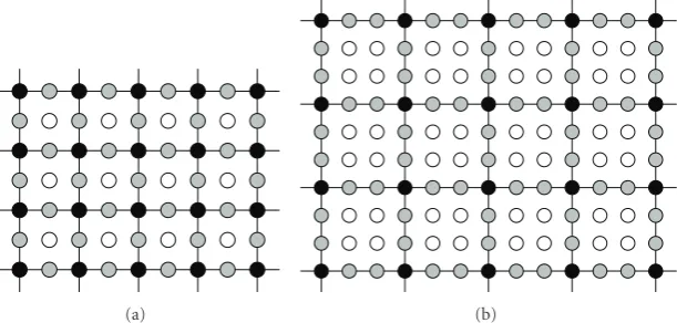
(a) (b)
Figure1: Production of LR images using subsampling: (a)κ=2, and (b)κ=3.
Since human visual system is strongly sensitive to the variations in intensity, an effective scheme that deals with spatial sharpness and edges is very useful to improve the quality of enlarged HR images. This study proposes an effi -cient interpolation algorithm comprising two main stages. In the first stage, an intelligent framework that combines fuzzy inference system and particle swarm optimization is adopted to restore the aligned pixels. In the second stage, the interior pixels are obtained via extending the edge properties of their neighbors. Experimental results demonstrate that the proposed method certainly achieves good capacity for enhancing spatial resolution of images.
This paper is organized as follows. Section 2 intro-duces the proposed two-stage interpolation algorithm in detail. Based on particle swarm optimization technique,
Section 3 presents a learning procedure to determine the critical parameters of the presented fuzzy inference system.
Section 4demonstrates the experimental results presented in numerical comparisons and visual illustrations. Final, a short conclusion is made inSection 5.
2. Two-Stage Interpolation Algorithm
2.1. Basic Concepts. Assume that a given LR imageILRof size
W×His to be enlarged into an HR imageIHRof sizeκW×
κH, whereκis a predefined magnification factor (MF). The LR image is generally treated as a subsampled version from its associated HR image. Figure 1 illustrates two standard examples of the production of LR images by subsampling for MFs κ = 2 and κ = 3, in which the black dots represent the preserved pixels in the LR image and the other dots represent lost pixels. The HR image is reconstructed in two interpolative stages: (1) thealigned pixels(gray dots in
Figure 1) along each dimension are estimated, and (2) the
interior pixels (white dots in Figure 1) are estimated. The following two subsections present the proposed two-stage interpolation algorithm.
2.2. The First Stage: Estimating Aligned Pixels. Figures 2(a)
and2(b)depict the aligned pixels located at (x+u,y) and (x,y+v) in unit division [x,x+ 1]×[y,y+ 1], respectively.
Take Figure 2(a) as an example to describe the process of estimating aligned pixels. Letfx,y∈ILRdenote the pixel value
at position (x,y), wherex=1, 2,. . .,W, andy=1, 2,. . .,H. The linear interpolation method yields the interpolated value of a specific point (x+u,y) as
fx+u,y=(1−u)fx,y+u fx+1,y, (1)
where u ∈ (0, 1) is the normalized Euclidean distance. For an arbitrary MF κ, u = ε/κ for ε = 1, 2,. . .,κ −1. However, the sharp details in reconstructed HR images are usually destroyed because the linear interpolation greatly suffers from blurring effects. Figure 3demonstrates a one-dimensional example of a blurred edge when linear interpo-lation is adopted, in which the original HR data in (a) are first subsampled into the decimated LR data in (b) and are then reconstructed to meet the original resolution in (c).
To introduce the novel contribution of this work,
Figure 4plots the pixels of interest and presents the impor-tant notation. As indicated in Figure 4, the interpolated result fx+udoes not accurately represent the original value fx+u, as an interpolation error of ex+u = |fx+u − fx+u|
exists. Intuitively, reducing the weight of sample fx(located
on the sharp side in Figure 4) and increasing the weight of sample fx+1 (located on the smooth side in Figure 4)
can effectively reduce this undesired interpolation error. Restated, the gradient measurement of each sample of interest helps in accurately estimating the interpolated result. Consequently, this subsection introduces a novel scheme that utilizes the gradients of sampling nodesx and (x+ 1) to obtain new weights of samples fx and fx+1. However,
the method for calculating (or modifying) weights is just a linguistic manner since neither a deterministic approach nor a mathematical derivation has been given. Fuzzy techniques have been extensively adopted in identifying unknown models or systems. Therefore, this study is the first to develop a fuzzy inference system (FIS) for deriving the weight of each neighboring sample.
Letℵ4denote the four corner pixels of the unit division
[x,x+1]×[y,y+1], such thatℵ4= {(i,j)|i∈ {x,x+1}; j∈
{y,y+1}}. Letgd[n], which is called the gradient component
(x,y) (x+ 1,y)
(x+u,y)
(x,y+ 1) (x+ 1,y+ 1) (a)
(x,y) (x+ 1,y)
(x,y+v)
(x,y+ 1) (x+ 1,y+ 1) (b)
(x,y) (x+ 1,y)
(x+u,y+v)
(x,y+ 1) (x+ 1,y+ 1) (c)
Figure2: Three cases of interpolation: (a) aligned pixel onx-axis, (b) aligned pixel ony-axis, and (c) interior pixel.
(a) (b)
Interpolated
(c)
Figure3: Blurring effect of linear interpolation in one-dimensional case: (a) original HR data points, (b) LR data by subsampling, and (c)
recovered data by linear interpolation.
fx+u fx+1 fx+2
ex+u
fx+u
fx−1
u fx
x−1 x x+u x+ 1 x+ 2 Figure 4: One-dimensional example of the conventional linear interpolation.
variable of the proposed FIS:
gd[n]=
⎧ ⎪ ⎪ ⎨ ⎪ ⎪ ⎩
fi+1,j−fi−1,j, ifd=1,
fi,j+1−fi,j−1, ifd=2,
(2)
wheren=(i,j) is selected from the corner pixelsℵ4. Define a
weighting factorτd[n] as the consequent variable; this factor
will be used to determine the weights of the considered pixels. Now, the modification rules are first constructed in linguistic
terms. For example, IF gradient is large (or small),THEN weighting factor is small(or large).
Hence, therth fuzzy rule is written in the following form:
Ruler: IFgd[n] isAr, THENτd[n] isBΓ−r+1, (3)
where r = 1, 2,. . .,Γ, and Γ is the total number of fuzzy rules, andAr andBΓ−r+1 are selected from{A1,A2,. . .,AΓ}
and{B1,B2,. . .,BΓ}, respectively (Figure 5). When gd[n] is
inputted to the FIS, the derived outputτd[n] is calculated via
fuzzy inference and defuzzification as follows:
τd[n]=
τd[n]·B(τd[n])
B(τ
d[n])
,
B(τd[n])= max
μ=1,2,...,Γ min
Aμ(τd[n]),BΓ−μ+1(τd[n])
.
(4)
As illustrated in Figure 2(a), the interpolated value of the aligned pixel (x+u,y) is calculated by
fx+u,y=τ1
[n1]
ω1
(1−u)fx,y+τ1
[n2]
ω1
u fx+1,y, (5)
whereω1 = τ1[n1](1−u) +τ1[n2]u, andn1 = (x,y) and
Me m b er sh ip d eg re
e A1 A2 A3 · · · AΓ−1 AΓ
gd[n]
α2
α1 αΓ−1 αΓ L−1 (a) Me m b er sh ip d eg re
e B1 B2 B3 · · · BΓ−1 BΓ
τd[n]
β2
β1 βΓ−1 βΓ
(b)
Figure5: Partitioned fuzzy sets of: (a) premise variable, and (b) consequent variable.
D4
D2
D3
D1
Figure6: Four directions of an edge.
inFigure 2(b), the interpolated value of the pixel (x,y+v) is calculated by
fx,y+v= τ2
[n1]
ω2
(1−v)fx,y+τ2
[n3]
ω2 v fx,y+1
, (6)
whereω2 = τ2[n1](1−v) +τ2[n3]v, andn3 = (x,y+ 1).
Therefore, the aligned pixels that were lost in LR images are restored using (5) and (6).
In brief, the first interpolative stage is proposed for estimating the aligned pixels from their neighbors that were preserved in LR images. By combining gradient components and fuzzy theory, the accuracy of interpolated values is certainly improved.
2.3. The Second Stage: Estimating Interior Pixels. The second stage presented in this subsection is employed to estimate the values of interior pixels that are marked as white dots in Figure 1. Since edge features are critical to representing the local characteristics of an image, the interior pixels are interpolated from their neighboring pixels by considering the
edge properties. Here, the neighboring pixels may be either the preserved pixels in the given LR image (black dots in
Figure 1) or the aligned pixels that were estimated in the first stage (gray dots inFigure 1).Figure 2(c)presents an interior pixel located in the unit division [x,x+ 1]×[y,y+ 1], in which u = ε1/κand v = ε2/κforε1,ε2 = 1, 2,. . .,κ−1.
The edge strengths and orientations of all pixels inℵ4must
be obtained first. Thus, the edge components of a specified pixeln∈ ℵ4are calculated using
Ex(n)= −fi−1,j−1−2fi−1,j−fi−1,j+1
+ fi+1,j−1+ 2fi+1,j+fi+1,j+1,
Ey(n)= −fi−1,j−1−2fi,j−1−fi+1,j−1
+ fi−1,j+1+ 2fi,j+1+fi+1,j+1.
(7)
Accordingly, the edge strength and orientation of n are obtained as follows:
E(n)= |Ex(n)|+Ey(n),
θ(n)=tan−1
Ex(n)
Ey(n)
.
(8)
For an interior pixel (x+u,y+v), the edge strength caused by a specific pixelnis defined as
Ξx+u,y+v(n)=(1− |x+u−i|)
1−y+v−jE(n). (9)
The pixel inℵ4that has maximal edge strength impacting on
interior pixel (x+u,y+v) is then selected as the dominant pixeln:
n= arg
n∈ℵ4
maxΞx+u,y+v(n)
. (10)
Base on the assumption that the edge orientation of an interior pixel (x+u,y+v) is directly designated as that of the dominant pixel, the orientation of (x+u,y+v) is defined asθ(n). Then,θ(n) is quantized in four ordinary directions
Dλ(λ=1, 2, 3, 4), as shown inFigure 6. Hence, the value of an
interior pixel is interpolated based on different orientations (along the direction with maximal edge strength) and is given in the following cases, where each case corresponds a specific direction.
Case 1. When the direction of the interior pixel is D1 as
shown inFigure 7(a), the interpolated pixel value is obtained from
fx+u,y+v=(1−u)fx,y+v+u fx+1,y+v. (11)
Case 2. When the direction of the interior pixel is D3 as
shown inFigure 7(b), the interpolated pixel value is obtained from
u
(x,y+v)
1−u
(x+ 1,y+v)
(a)
v
1−v
(x+u,y)
(x+u,y+ 1)
(b)
u+v <1 fΨ
rΨ
rΦ
fΦ
rΦ
rΨ
fΨ
rΨ
rΦ
fΦ
u+v >1 (c)
u > v fΦ
rΦ rΦ
fΦ
rΦ
rΨ
fΨ
rΨ
rΨ
fΨ
u < v
(d) Figure7: Four classical cases for interpolating interior pixels.
Case 3. When the direction of the interior pixel is D2 as
shown inFigure 7(c), the pixel value is linearly interpolated from those of its neighbors:
fx+u,y+v= rΨ
rΦ+rΨfΦ+
rΦ
rΦ+rΨfΨ, (13)
where fΦ, fΨ, rΦ, and rΨ are obtained by considering the following three subcases.
Subcase 3.1. fΦ = fx,y+1, fΨ = fx+1,y,rΦ =
u2+ (1−v)2,
rΨ=(1−u)2+v2,asu+v=1.
Subcase 3.2. fΦ= fx,y+u+v, fΨ= fx+u+v,y,rΦ=u,rΨ=v, as
u+v <1.
Subcase 3.3. fΦ= fx+u+v−1,y+1, fΨ= fx+1,y+u+v−1,rΦ=1−v,
rΨ=1−u, asu+v >1.
Case 4. When the direction of the interior pixel is D4 as
shown in Figure 7(d), the pixel value is interpolated using (13), and subcases are described below.
Subcase 4.1. fΦ = fx,y, fΨ = fx+1,y+1,rΦ =
√
u2+v2,rΨ =
(1−u)2+ (1−v)2, asu=v.
Subcase 4.2. fΦ = fx+u−v,y, fΨ= fx+1,y−u+v+1,rΦ =v,rΨ =
1−u, asu > v.
Subcase 4.3. fΦ = fx,y−u+v, fΨ = fx+u−v+1,y+1,rΦ =u,rΨ =
1−v, asu < v.
The two main stages of the estimation of the aligned pixels based on local gradients and of the estimation of interior pixels using edge properties of neighbors have now been introduced. Consequently, the proposed two-stage interpolation algorithm is carried out by implementing these two stages in correct order.
3. Parameters Determination
(a) (b) (c)
(d) (e) (f)
Figure8: A set of test images: (a) Airplane, (b) Boats, (c) Cameraman, (d) Lena, (e) MRI, and (f) Peppers.
Moreover, some critical parameters must still be determined. They include{α1,α2,. . .,αΓ},{β1,β2,. . .,βΓ}andΓ. Suppose
that{α1,α2,. . .,αΓ}and{β1,β2,. . .,βΓ}are equally spaced in
the intervals [0,αΓ] and [0, 1], respectively, such thatα1=0,
β1 = 0 andβΓ = 1. The parameters are now reformulated
as
αm=m−
1
Γ−1αΓ, βm=
m−1
Γ−1, form=1, 2,. . .,Γ. (14)
Therefore, the total number of parameters is significantly reduced, and only two parameters,αΓ andΓ, need now be considered. Next, the particle swarm optimization procedure is adopted to determine parameters.
Particle swarm optimization (PSO) is a population-based evolutionary algorithm that was inspired by the social behavior of biological organisms [29, 30], which is associated with an optimization search for solutions. As an optimization approach, the PSO algorithm provides an iteratively searching capability in which each particle moves through the multidimensional search space. Theth particle in the n-dimensional search space is specified by three components, which are its positionp = [p1,p2,. . .,pn],
its velocityv =[v1,v2,. . .,vn], and the best position that
it has achieved so farb =[b1,b2,. . .,bn] (for individual
best). Particles are initialized randomly and the particles then
move through the search space. In time stept, the position of theth particlep ( = 1, 2,. . .,M) is updated by adding a
velocity vectorvi, whereM is the total number of particles
in the swarm. In standard PSO, the velocity and position are updated using (15):
v(t+ 1)=w(t)v(t) +ρ1
b(t)−p(t)
+ρ2
b(t)−p(t)
,
p(t+ 1)=p(t) +v(t+ 1),
(15)
wherebis the best position found so far among all particles in the swarm (for global best);ρ1andρ2are random numbers
distributed in the interval [0, 1] that are generated in each time step.
Let fx,y ∈ IHR and fx,y ∈ IHR represent the pixel
values in the original image and in the interpolated image, respectively. The peak signal-to-noise ratio (PSNR) between the two images, given by (16), is adopted as the fitness functionJto evaluate the solution for theth particle:
PSNR=10·log10(L−1)
2
MSE , (16)
MSE= 1
κW·κH
κW
x=1 κH
y=1
fx,y−fx,y
2
(a) (b) (c)
(d) (e) (f)
(g) (h) (i)
(j) (k) (l)
Figure9: Close-up part of (a) originalLenaimage and its reproduced version interpolated by (b) Nearest Neighbor, (c) Bilinear, (d) WaDi-Bil, (e) Adaptive-WaDi-Bil, (f) CFLS, (g) ESIF, (h) EDI, (i) EOA, (j) LAZA, and (k) SAI and (l) the proposed method.
foreach time stept do forth particle in swarmdo
Update the positionpusing (14).
Calculate fitness functionJ.
Update the best positionsbandb.
end for end for
Algorithm1: Main procedure in particle swarm optimization.
whereL=28=256 for 8-bit images;κWandκHdenote the
width and the height of the interpolated images. The main procedure in particle swarm optimization is summarized as inAlgorithm 1.
Assume that an integer-valued particlep = [p1,p2]
moves through a two-dimensional search space that is bounded in [0,L−1]×[1,Γmax]. The terms p1 and p2
stand for parametersαΓ andΓ, respectively. To reduce the computational burden, the maximal number of fuzzy rules is set toΓmax =15. The values optimized by PSO areαΓ =
136 and Γ = 9. Consequently, the critical parameters that characterize the proposed FIS are completely determined using (14).
4. Experimental Results
(a) (b) (c)
(d) (e) (f)
Figure10: Close-up part of reproducedBoatsimage processed by six well-performing methods: (a) WaDi-Bil, (b) Adaptive-Bil, (c) ESIF, (d) LAZA, (e) SAI, and (f) the proposed method.
Table1: Numerical results presented in PSNRs between different interpolation methods.
Methods Peak signal-to-noise ratios (in dBs) for different test images
Airplane Boats Cameraman Lena MRI Peppers
Nearest neighbor 27.19 26.11 27.48 29.10 31.32 29.52
Bilinear 32.75 30.36 34.14 35.65 41.10 35.27
WaDi-Bil [14] 33.22 30.50 35.42 36.19 42.63 35.73
Adaptive-Bil [13] 33.15 30.41 34.35 35.85 41.12 36.22
CFLS [26] 31.74 29.84 33.14 34.09 36.52 33.91
ESIF [1] 32.89 30.43 34.68 35.89 42.64 35.67
EDI [2] 32.88 29.96 33.10 35.60 41.54 35.75
EOA [3] 31.35 29.37 34.05 34.24 38.79 33.95
LAZA [5] 32.75 30.42 34.24 35.91 41.13 35.47
SAI [6] 32.86 30.38 35.06 35.84 42.65 36.40
Proposed method 33.67 30.86 36.27 36.85 43.44 36.42
this experiment because some of the compared methods have been proposed for use in 2× image enlargement applications [2,3,5,6].Table 1 numerically compares the PSNR values obtained using different methods. Notably, the proposed two-stage interpolation algorithm outper-forms other methods by an average of 0.7–5 dB. The SAI approach resulted in acceptable performance but cost
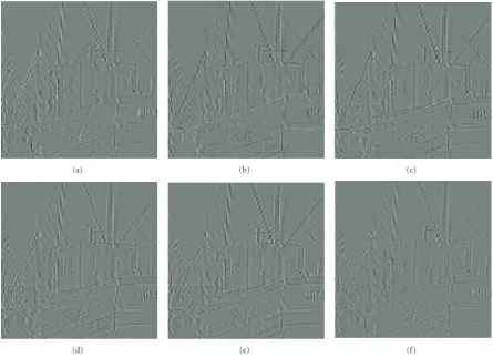
(a) (b) (c)
(d) (e) (f)
Figure11: Error image with respect to original image forFigure 10.
Table2: Numerical results presented in SSIMs between different interpolation methods.
Methods Structural similarity for different test images
Airplane Boats Cameraman Lena MRI Peppers
Nearest Neighbor 0.9508 0.9157 0.9640 0.9456 0.981 0.9536
Bilinear 0.9816 0.9594 0.9902 0.9830 0.9973 0.9819
WaDi-Bil [14] 0.9825 0.9602 0.9917 0.9838 0.9977 0.9825
Adaptive-Bil [13] 0.9820 0.9558 0.9895 0.9827 0.9977 0.9827
CFLS [26] 0.9824 0.9687 0.9831 0.9820 0.9934 0.9844
ESIF [1] 0.9818 0.9595 0.9907 0.9831 0.9977 0.9823
EDI [2] 0.9816 0.9593 0.9836 0.9829 0.9973 0.9825
EOA [3] 0.9810 0.9584 0.9881 0.9821 0.9857 0.9816
LAZA [5] 0.9816 0.9555 0.9908 0.9830 0.9978 0.9826
SAI [6] 0.9830 0.9603 0.9926 0.9832 0.9981 0.9835
Proposed Method 0.9836 0.9614 0.9929 0.9851 0.9985 0.9834
Figure 9 presents a close-up part of the Lena image, interpolated using different image interpolation approaches. As demonstrated, the nearest neighbor method yields block-ing artifacts; the bilinear and CFLS methods blur the details and edges, but the proposed algorithm preserves them. Figure 10 displays another simulation of the Boats
image, which contains many edges. In this figure, six well-performing interpolation methods were demonstrated. To compare clearly the performance of different methods,
Figure 11 illustrates an error map of the interpolated
5. Conclusions
This study has presented an efficient interpolation method for image processing applications. The HR images are reproduced by estimating the values of aligned pixels and then estimating the values of interior pixels. The first stage deals with the lost pixels using an intelligent scheme that combines fuzzy logic and particle swarm optimization. The grayscale values of aligned pixels are interpolated by using the optimized fuzzy inference system whose input is the local gradient information. In the second interpolative stage, the lost pixels in an interior region are restored from the edge fea-tures of their neighbors. Numerical comparisons verify the effectiveness of the proposed interpolation algorithm applied to different images. Close-up observations and error maps demonstrate the superiority of the proposed algorithm over other methods in restoring local edges. The proposed two-stage interpolation algorithm yields substantially improved performance of image zooming and enlargement.
Acknowledgments
The authors would like to thank the National Science Council of the Republic of China, Taiwan, for financially supporting this research under the Grant NSC-96-2221-E-027-136. The authors also thank the National Central Uni-versity, Taiwan, for providing website services. Please refer to
http://www.ee.ncu.edu.tw/∼fuzzylab/ExpResults/ (National Central University) for downloading the results and related materials.
References
[1] S. Carrato, G. Ramponi, and S. Marsi, “Simple edge-sensitive image interpolation filter,” in Proceedings of the IEEE Inter-national Conference on Image Processing, vol. 3, pp. 711–714, 1996.
[2] X. Li and M. T. Orchard, “New edge-directed interpolation,” IEEE Transactions on Image Processing, vol. 10, no. 10, pp. 1521–1527, 2001.
[3] M.-J. Chen, C.-H. Huang, and W.-L. Lee, “A fast edge-oriented algorithm for image interpolation,”Image and Vision Computing, vol. 23, no. 9, pp. 791–798, 2005.
[4] L. Zhang and X. Wu, “An edge-guided image interpolation algorithm via directional filtering and data fusion,” IEEE Transactions on Image Processing, vol. 15, no. 8, pp. 2226–2238, 2006.
[5] S. Battiato, G. Gallo, and F. Stanco, “A locally adaptive zooming algorithm for digital images,” Image and Vision Computing, vol. 20, no. 11, pp. 805–812, 2002.
[6] X. Zhang and X. Wu, “Image interpolation by adaptive 2-D autoregressive modeling and soft-decision estimation,”IEEE Transactions on Image Processing, vol. 17, no. 6, pp. 887–896, 2008.
[7] D. D. Muresan and T. W. Parks, “Adaptively quadratic (AQua) image interpolation,”IEEE Transactions on Image Processing, vol. 13, no. 5, pp. 690–698, 2004.
[8] T. M. Lehmann, C. G¨onner, and K. Spitzer, “Surveys: interpolation methods in medical image processing,” IEEE Transactions on Medical Imaging, vol. 18, no. 11, pp. 1049– 1075, 1999.
[9] P. Th´evenaz, T. Blu, and M. Unser, “Interpolation revisited,” IEEE Transactions on Medical Imaging, vol. 19, no. 7, pp. 739– 758, 2000.
[10] R. G. Keys, “Cubic convolution interpolation for digital image processing,”IEEE Transactions on Acoustics, Speech, and Signal Processing, vol. 29, no. 6, pp. 1153–1160, 1981.
[11] S. E. Reichenbach and F. Geng, “Two-cimensional cubic convolution,”IEEE Transactions on Image Processing, vol. 12, no. 8, pp. 857–865, 2003.
[12] J. Z. Shi and S. E. Reichenbach, “Image interpolation by two-dimensional parametric cubic convolution,”IEEE Transactions on Image Processing, vol. 15, no. 7, pp. 1857–1870, 2006. [13] J. W. Hwang and H. S. Lee, “Adaptive image interpolation
based on local gradient features,” IEEE Signal Processing Letters, vol. 11, no. 3, pp. 359–362, 2004.
[14] G. Ramponi, “Warped distance for space-variant linear image interpolation,”IEEE Transactions on Image Processing, vol. 8, no. 5, pp. 629–639, 1999.
[15] Q. Wang and R. K. Ward, “A new orientation-adaptive interpolation method,”IEEE Transactions on Image Processing, vol. 16, no. 4, pp. 889–900, 2007.
[16] T. Hermosilla, E. Bermejo, A. Balaguer, and L. A. Ruiz, “Non-linear fourth-order image interpolation for subpixel edge detection and localization,”Image and Vision Computing, vol. 26, no. 9, pp. 1240–1248, 2008.
[17] T. Sigitani, Y. Iiguni, and H. Maeda, “Image interpolation for progressive transmission by using radial basis function networks,”IEEE Transactions on Neural Networks, vol. 10, no. 2, pp. 381–390, 1999.
[18] N. Plaziac, “Image interpolation using neural networks,”IEEE Transactions on Image Processing, vol. 8, no. 11, pp. 1647–1651, 1999.
[19] A. Amanatiadis, I. Andreadis, and K. Konstantinidis, “Design and implementation of a fuzzy area-based image-scaling technique,”IEEE Transactions on Instrumentation and Mea-surement, vol. 57, no. 8, pp. 1504–1513, 2008.
[20] L. Ma, Y. Shen, and J. Ma, “Local spatial properties based image interpolation scheme using SVMs,”Journal of Systems Engineering and Electronics, vol. 19, no. 3, pp. 618–623, 2008. [21] D. G. Sheppard, K. Panchapakesan, A. Bilgin, B. R. Hunt,
and M. W. Marcellin, “Lapped nonlinear interpolative vector quantization and image super-resolution,”IEEE Transactions on Image Processing, vol. 9, no. 2, pp. 295–298, 2000.
[22] S.-H. Hong, R.-H. Park, S. Yang, and J.-Y. Kim, “Image inter-polation using interpolative classified vector quantization,” Image and Vision Computing, vol. 26, no. 2, pp. 228–239, 2008. [23] A. Temizel and T. Vlachos, “Wavelet domain image resolution enhancement,” IEE Proceedings: Vision, Image and Signal Processing, vol. 153, no. 1, pp. 25–30, 2006.
[24] S. G. Chang, Z. Cvetkovi´c, and M. Vetterli, “Locally adaptive wavelet-based image interpolation,” IEEE Transactions on Image Processing, vol. 15, no. 6, pp. 1471–1485, 2006. [25] F. Ar`andiga, R. Donat, and P. Mulet, “Adaptive interpolation
of images,”Signal Processing, vol. 83, no. 2, pp. 459–464, 2003. [26] H. Yoo, “Closed-form least-squares technique for adaptive linear image interpolation,”Electronics Letters, vol. 43, no. 4, pp. 210–212, 2007.
[27] Y. Cha and S. Kim, “The error-amended sharp edge (EASE) scheme for image zooming,” IEEE Transactions on Image Processing, vol. 16, no. 6, pp. 1496–1505, 2007.
[29] J. Kennedy, “Particle swarm optimization,” inProceedings of the IEEE International Conference on Neural Networks (ICNN ’95), vol. 4, pp. 1942–1948, Australia, November 1995. [30] R. Eberhart and J. Kennedy, “A new optimizer using particle
swarm theory,” inProceedings of the 6th International Sympo-sium on Micro Machine and Human Science (MHS ’95), pp. 39–43, Nagoya, Japan, October 1995.