An FPGA-Based People Detection System

(1)

An FPGA-Based People Detection System

Vinod Nair

Centre for Intelligent Machines, McGill University, Montreal, QC, Canada H3A 2A7 Email:[email protected]

Pierre-Olivier Laprise

James J. Clark

Received 15 September 2003; Revised 12 August 2004

This paper presents an FPGA-based system for detecting people from video. The system is designed to use JPEG-compressed frames from a network camera. Unlike previous approaches that use techniques such as background subtraction and motion detection, we use a machine-learning-based approach to train an accurate detector. We address the hardware design challenges involved in implementing such a detector, along with JPEG decompression, on an FPGA. We also present an algorithm that eﬃciently combines JPEG decompression with the detection process. This algorithm carries out the inverse DCT step of JPEG decompression only partially. Therefore, it is computationally more eﬃcient and simpler to implement, and it takes up less space on the chip than the full inverse DCT algorithm. The system is demonstrated on an automated video surveillance application and the performance of both hardware and software implementations is analyzed. The results show that the system can detect people accurately at a rate of about 2.5 frames per second on a Virtex-II 2V1000 using a MicroBlaze processor running at 75 MHz, communicating with dedicated hardware over FSL links.

Keywords and phrases:computer vision, FPGA, people detection, smart camera.

1. INTRODUCTION

This paper describes a system for detecting people in images, implemented on a field-programmable gate array (FPGA). People detection is an important subtask in many computer vision applications, such as automated video surveillance, human activity recognition, and smart room systems. The output of a people detector can be used, for instance, to in-fer a person’s location in a scene or to track the person over time. Such location and tracking data can then be analyzed to automatically generate a human-understandable descrip-tion of what the person might be doing, or raise an alarm if the person’s behavior seems unusual.

Many vision applications often involve a large number of cameras. For example, wide-area surveillance networks use tens to hundreds of cameras to monitor many diﬀerent scenes. Sending the video from all the cameras to a single central workstation for processing can be prohibitively ex-pensive because of the need for high-bandwidth transmis-sion. An attractive alternative is to perform the processing on

the camera itself with a fast and inexpensive FPGA chip. In recent years, FPGA technology has become increasingly pow-erful, less expensive, and more practical for use in real-time vision applications. Our long-term goal is to build a frame-work in which a large number of cameras cooperate to carry out a collective task (such as surveillance), with each per-forming its own FPGA-based video analysis, and exchanging high-level, low-bandwidth information over a network.

As a first step toward such a framework, we have im-plemented a single-camera people detection system on an FPGA. The system is demonstrated on a corridor surveillance application. Here the task is to detect people appearing in an oﬃce corridor from the JPEG-compressed frames provided by a fixed network camera. Example frames from the camera are shown inFigure 1. By “detecting people,” we mean com-puting an accurate bounding box for each fully visible person in a frame.

(2)

(a) (b) (c) (d)

Figure1: Example images of the scene under surveillance.

as background subtraction or motion detection. Such tech-niques are relatively easy to port on to a chip because they mainly involve simply differencing images. An example of this approach implemented on an FPGA is [1]. However, de-tection methods based on background subtraction or motion can often fail because of sudden changes in scene illumina-tion, shadows, similar pixel values shared by the foreground and the background, and other difficult background model-ing problems. As explained later, the learned classifier-based approach is not affected by these problems and therefore can be more robust and accurate. The detection algorithm we use is developed by Viola and Jones [2]. This algorithm is de-scribed inSection 3.

Such an approach to people detection is also an unusual choice for FPGA implementation, since vision and image processing algorithms successfully ported to FPGAs tend to be of the data-streaming or small-neighbourhood filter va-riety. Many of the more complex algorithms are frequently deemed unsuitable for FPGA implementation due to the ne-cessity for floating-point operations or because of the lim-ited amount of rapid, on-chip memory compared to the vol-ume of data that needs to be processed. Instead of avoiding these problems by changing algorithms, we explore methods to mitigate their eﬀects on system performance, thereby ex-panding the range of algorithms suitable for FPGA. Details of the firmware implementation of the people detection al-gorithm and JPEG decompression are provided in Sections4 and5.

Another contribution of our work is an algorithm that combines the JPEG decompression with the detection algo-rithm in a hardware-friendly manner. The Viola-Jones detec-tor needs to compute an “integral image” of a video frame in order to detect people in that frame. We present a method for computing an approximate integral image directly from JPEG, without computing the fully decompressed frame. This method is simpler to implement on an FPGA than a full-fledged JPEG decompressor, it takes up less space on the chip, and it requires fewer computations compared to calcu-lating the integral image from a fully decompressed frame. The algorithm for approximating the integral image is de-scribed inSection 6. The firmware implementation details of the approximation algorithm are given inSection 7.

An overview of the system we have implemented is given inSection 2. Accuracy results for the trained detector are pre-sented inSection 8.

2. SYSTEM OVERVIEW

People detection is rarely an end in itself, but more often an intermediate step in a higher-complexity algorithm. Our approach to this problem is to have multiple, independent camera-based processing units communicating high-level in-formation about a scene instead of raw data. In the more complex applications, one can expect that the camera net-work will be highly heterogeneous, with cameras implement-ing low-level algorithms and passimplement-ing on their results to cam-eras with higher-level algorithms, in an analogous manner to the multiple levels of processing found in the human visual system.

To simplify the design of the various modules that would be required in such a network, it is important to have a pow-erful yet flexible and adaptive framework. Cost is also a fac-tor due to the large number of nodes that should compose the network. In fact, it should be expected that the system’s true power comes from distributing the processing load over multiple nodes rather than from the processing power of the individual nodes in the network.

The desire to have as many nodes as possible combined with the requirement that each node be capable of executing moderately complex algorithms in real time were the guid-ing constraints in node design. This required the solution to be as cost-eﬀective as possible, yet still capable of high-performance image processing. Reconfigurable computing architectures have shown time and again an ability toward accelerating image processing tasks [3,4, 5,6,7], and are therefore ideally suited to this application.

Current advances in FPGA technologies are making it possible to envisage the design of a system on a pro-grammable chip (SOPC), in which all the components which previously required separate components on a printed circuit board (PCB) can be fit onto a single FPGA chip. This allows embedding of a microprocessor on the FPGA itself instead of placing it alongside on a PCB. Xilinx provides two avenues to this eﬀect, the MicroBlaze soft processor for the Virtex-II family of chips, and the IBM PowerPC processor embedded into the Virtex-II Pro family of FPGAs.

(3)

the parallelism oﬀered by custom hardware designs. This also permits a tight, optimized coupling between the data pro-cessing elements and the data source, such as the camera or memory.

The more conventional approach to a reconfigurable computing architecture is to have a dedicated micro-proc-essor ASIC using an FPGA as a reconfigurable coproces-sor. Such a configuration has many advantages, namely, per-formance, but it sacrifices some of the flexibility and cost-eﬀectiveness of a single-chip solution.

Other limitations were imposed by the prototyping plat-form that was initially chosen. Although the video input will be tightly coupled to the FPGA in future versions, no read-ily available commercial board was found to satisfy this re-quirement along with all the others. The chosen prototyping board was Insight Memec’s V2MB1000 board, which pro-vides a large variety of I/O, such as LVDS pins, which will be necessary for high-speed board-to-board communication. It was decided that the actual source of the video feed had lim-ited impact on the functionality of the system, and that rea-sonable performance estimates could still be garnered from the implementation.

For the node application example described in this pa-per, the source images were gathered from a network camera with onboard JPEG compression and HTTP server over Eth-ernet, Axis Communication’s NetCam 200+. Unfortunately, the live stream from this camera is limited to 1 352×288 pixel frame per second. Having a JPEG video source allowed exploration into the possibilities of integrating real-time im-age compression and decompression into a standard com-puter vision algorithm. Integrating compression and decom-pression of a data stream into the application (whether us-ing JPEG or other means) is an important step toward re-ducing the bandwidth required in transferring data between network nodes or even between the FPGA and memory. In fact, hardware implementations of computer vision and image processing algorithms are more often limited by the speed of their I/O than by the speed at which they are able to process data, which is why most of the algorithms im-plemented in hardware are of the streaming filter variety, where memory demands are limited. Compressing the data that is to be transferred therefore has the potential of im-proving the system performance by increasing the eﬀective bandwidth as long as compression and decompression of the data have a limited eﬀect on the speed of the overall system.

The global system organization can be seen inFigure 2. Execution starts when the MicroBlaze processor retrieves the JPEG image from the network camera using HTTP over Eth-ernet. The JPEG data is separated from the header and passed to the JPEG decoder and people detection module, which is described in more detail in this paper. The integral im-age (an intermediate format needed by the algorithm) is stored in DDR SDRAM for the use of the application-specific firmware, to which it is tightly coupled with a controller op-timized for this specific application to minimize overhead costs.

ASFW (people detector)

FSL bus

uBlaze

(Ethernet + control) BRAM

DDR SDRAM

Ctrl

Instr. bus OPB

UART GPIO Ethernet (Integral image)

Data bus

Figure2: Organization of IP cores on the FPGA for a single-chip solution.

3. THE PEOPLE DETECTION ALGORITHM

People detection is performed using the Viola-Jones algo-rithm, which is a general method that can be used to learn a detector for any type of object. Here we give a brief sum-mary of the algorithm as it applies to our work. For a full description, see [2].

3.1. Viola-Jones detection algorithm

The basic detection strategy of the Viola-Jones algorithm consists of two steps. First, an image classifier is trained to ac-curately classify cropped people and nonpeople images (ex-amples of such images are shown in Figure 3). Then, in-stances of the “people” object are detected in a given video frame by “scanning” the frame with the classifier. Scanning involves sliding a window over the frame, and the classifier is asked to label the subimage defined by each window posi-tion as either “people” or “nonpeople.” When the window is right on top of a person in the image, the classifier will (hope-fully) label it as “people” and thus detect the person. People of different sizes can be detected by scanning at many diff er-ent window scales. Note that this strategy does not make any assumptions about the scene background or interframe dif-ference, so it is not affected by problems such as sudden illu-mination changes, shadows, and other difficult background modeling problems that commonly plague detection meth-ods based on background subtraction or motion.

(4)

Figure3: Examples of cropped people and nonpeople images.

Figure4: The three feature types used by the people detector.

diﬀerent orientations. For each type, thousands of features can be defined by varying the location and the size of the fea-ture within the cropped image. We use a total of 21804 such features for all three types. Therefore, during training, each cropped image is represented as a 21804-dimensional feature vector.

Most of these features are likely to be useless for classi-fying people and nonpeople images. The AdaBoost learning algorithm is used to select the few features that are actually useful for accurate classification. The final classifier obtained at the end of the training contains only a small fraction of the initial pool of features. So when a frame is scanned using the classifier, onlyO(100) features have to be computed per subimage, rather than all 21804.

These features can be computed rapidly using what Viola and Jones call the “integral image.” Given a grayscale image, its integral image is a matrix whose element at therth row andcth column is the sum of all pixels up to and including rowr and column cof the grayscale image. Once the inte-gral image is computed, the sum of any rectangular region of pixels in the image can be computed with only four addi-tions, as explained in [2]. This means that the value of a local image feature can be computed very quickly at any scale. So when scanning a frame for people at various scales, it is not necessary to resize the frame at those scales with an image pyramid. Instead, the classifier itself can be “resized” sim-ply by rescaling the features it uses. As a result, scanning is

computationally much more eﬃcient than with the pyramid approach. What makes this algorithm particularly attractive for hardware implementation is that most of the arithmetic operations involved during detection are additions.

To improve the speed of the detection process, a cascade of strong classifiers is constructed, instead of just one strong classifier. This strategy is based on the observation that al-most all subimages encountered when scanning a frame be-long to the negative class (i.e., nonpeople). Therefore, the structure of an efficient classifier should be geared toward re-jecting negative instances as quickly as possible, with large amounts of classification effort expended only on the rare positive instances. To classify a subimage, it is passed through a cascade sequence of strong classifiers until one of them rejects it as a negative instance. If the subimage survives all stages of the cascade, then it is labeled as a positive in-stance. The further down the cascade a strong classifier is, the more features it contains. As a result, the small initial cas-cade stages quickly eliminate the “easy” nonpeople instances. More computational effort is required to reject the remain-ing, more ambiguous nonpeople instances by the subsequent larger stages. Although classifying a subimage as “people” re-quires evaluating all the features in the entire cascade, such subimages are rare. Therefore, the average number of fea-tures computed per subimage, which determines the overall speed of the detector, still remains fairly small.

The dimensions of the network camera frames we use are 352×288. Scanning is done only in a 216×288 rectangular region in the middle of the frame that corresponds to the part of the corridor where people actually appear. The size of the scan window is restricted to be a multiple of 16×48 (width×height). Allowed multiples go from 1.0 (16×48) to 6.0 (96×288) in increments of 0.25. The number of pixels by which the subwindow is shifted horizontally and vertically is computed as 25% of its width and height, respectively. In each frame, 3079 subimages have to be classified during scan-ning.

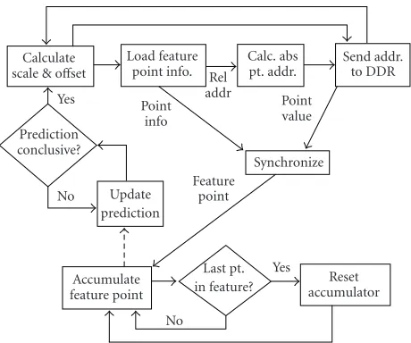
4. PEOPLE DETECTION IN FIRMWARE

(5)

Calculate scale & oﬀset

Load feature point info. _Rel

addr

Calc. abs pt. addr.

Send addr. to DDR Point

value Point

info Prediction

conclusive?

Synchronize Update

prediction

Feature point No

Yes

Accumulate feature point

Last pt.

in feature? _accumulatorReset No

Yes

Figure5: Flowchart for the firmware implementation of the people detection algorithm.

implementation’s flowchart is shown in Figure 5. Having stored the image in integral image format, the sum of pixels in a rectangular region of any size only requires the addition or subtraction of the region’s four corners. Therefore, all that is required to calculate a feature’s value is a simple accumula-tor circuit. Each accumulated point is either multiplied by±1 or±2, and the features that were used can have either 6 or 8 points of interest. The only difficulty stems from the limited amount of on-chip memory available. Since the integral im-age is much too large to fit on-chip, it must be stored in an ex-ternal memory, which is necessarily much slower to access. In the current implementation, the off-chip memory is a DDR SDRAM with a 16-bit data bus working at 100 MHz. This al-lows for a transfer rate which can never surpass 32 bits per 10 nanoseconds. With the targeted FPGA system clock speed also at 100 MHz, the system would be receiving at most one integral point per cycle, even without taking into account ad-dressing overhead and memory refresh times. Various meth-ods were considered in order to compress the integral im-age and allow greater throughput, but the necessity to access widely separate points in a pseudorandom order made this a difficult task. Given that we have a priori knowledge of the patterns with which data points can be fetched, it should be possible to optimize the memory controller for this applica-tion, for example, by inserting memory refreshes in natural pauses in the flow, but this would be far from trivial and is therefore left as future work.

Classifier training determines the position, size, and type of features that are required to detect a person. These val-ues are all given with respect to a 16×48 template window, which is then shifted and scaled to detect people of diﬀerent sizes in varying places in the image. The address of a point in external memory therefore depends both on its position in the template window, and on the template’s position and scale in the image at any given point in the scan. Training also determines the feature’s threshold, its weight in the stage, and

the global threshold for each stage. In order to minimize de-lays, this information should all be stored on-chip, but this can require a large amount of memory if one is not careful. Consequently, it is necessary to organize the information so as to most tightly pack it into the available memory formats. The first step is to determine the minimum required data width for each signal. This is simple for most signals, but some require more detailed analysis, and can usually be split into absolute and relative ranges. Analysis of absolute ranges is simply a question of finding the maximum and minimum values for a variable and scaling it to fit an integer of mini-mum size. An example of such a signal is the feature thresh-old, which is determined by the feature size and maximum pixel value, such that it can necessarily fit into 18 bits. How-ever, analysis of the training data shows that no threshold ever needs more than 15 bits. Since the system can be recon-figured through judicious use of parameters if this changes, the optimal size for a given training session can be used for storage.

Relative ranges, such as that of the feature weights, only have relevance one with respect to the others, and can be rep-resented as numbers of arbitrary precision between zero and one. These ranges can never be fully covered, but statistical analysis of the training results yields the error associated with a given data width. For example, normalizing the weights to 18-bit integers allows for all but 0.13% of the weights to have a unique value compared to the full floating-point represen-tation.

Once the data widths have been optimized, the signals which are always retrieved together can be packed into a sin-gle word in memory to reduce the number of memory ac-cesses. This mapping, however, should be encapsulated in such a way as to present the functional separations rather than the actual ones in order to facilitate code reuse and maintenance.

5. CALCULATING THE INTEGRAL IMAGE FROM JPEG

Computing the integral image of a grayscale frame is sim-ple (see [2] for details) if the frame is not compressed. In our case, however, it is compressed in JPEG format. The JPEG de-compression algorithm involves computing the inverse dis-crete cosine transform (DCT) [9], which requires nontriv-ial hardware resources and computational effort. Therefore, we seek to avoid computing the inverse DCT. It is possible to obtain the integral image directly from the DCT coeffi -cients because both the forward and inverse discrete cosine transforms are linear transformations, which means that the coefficients are linear combinations of pixel values and vice versa. So the pixel sums required in the integral image com-putation can be obtained through linear combinations of the DCT coefficients.

(6)

Huﬀman

decoder Dequantizer _DCT coeﬃcients

Direct method

Inverse

DCT Integrate

Grayscale image

Integral image JPEG

Figure6: Once the JPEG image’s DCT coeﬃcients are decoded, the standard method would be to perform an inverse DCT and integrate the resulting grayscale image. Instead, the integral image can be extracted directly from the coeﬃcients.

frame and its integral image contain the same amount of information, and the conversion between the integral and grayscale forms is trivial compared to the inverse DCT. Therefore, calculating the integral image directly from the DCT coeﬃcients requires about as much eﬀort as the in-verse DCT itself. However, it may be possible to directly compute anapproximateintegral image with fewer compu-tations.

5.1. Extraction of DCT coefficients

The extraction of DCT coefficients from a JPEG stream re-quires first that a Huffman-encoded value be decoded, which is then used to decode the bits in the stream which encode the coefficient’s actual value. This necessitates the use of a Huffman table which is transmitted with the image. How-ever, JPEG encoders (including the one used for this exper-iment) generally use the same Huffman table for all the im-ages that they generate. Having verified whether this is the case for a particular encoder, and with knowledge that all fu-ture images in the series will come from the same encoder, it is possible to only extract the table from the first image received or, in a prototyping environment, to hardcode the tables into the FPGA’s configuration bitstream. The quanti-zation tables used inSection 7may be treated in the same manner.

It was clear from the start that the speed at which the JPEG decoding module processes data would be limited at the input by the fact that the data is being sent over a 10/100 Ethernet line, which has a maximum transfer rate of 10 ns/bit, and at the output by the integral image module, which needs to write its results to external memory. There-fore, a simple serial lookup table approach to Huffman de-coding, such as the one described in [9], should be sufficient to meet data rate limitations at both ends. Once the Huffman decoding is complete, decoding the coefficient’s value and in-dex is relatively simple to do in parallel at a small additional cost in complexity. Simplified block diagrams of these mod-ules’ implementations can be seen in Figures7,8, and9.

Tests on a source image suggest that if the decoding hard-ware were only slightly limited by input speed (overhead of 2 cycles per 16 bits of data), the hardware should take approxi-mately 75 kcycles to treat a typical image, which translates to 1.5 milliseconds for a worst-case 20 nanoseconds minimum period. However, as will be seen inSection 7, most of this time can be absorbed by the calculation of the integral im-age, with a simple FIFO buﬀer to synchronize the modules.

6. AN EFFICIENT ALGORITHM FOR APPROXIMATING THE INTEGRAL IMAGE

We have developed an algorithm for calculating an approx-imate integral image that needs significantly fewer compu-tations and hardware resources than the inverse DCT. The basic idea is to compute the integral image exactly at some points in the image and then approximate it everywhere else by interpolation. The JPEG compression algorithm parti-tions a grayscale image into nonoverlapping 8×8 pixel blocks and computes the 64 DCT coefficients for each block. These coefficients can be obtained from the JPEG data by Huffman decoding and dequantization [9]. Since the DC coefficient of a block encodes the average pixel value of that block [10], the sum of all pixels in an 8×8 block can be calculated from its DC coefficient alone. Using all such local 8×8 block sums of an image, it is possible to compute the exact value of the inte-gral image at the bottom-right corner of every 8×8 block in the image, as shown by the example inFigure 10a. Suppose thatS1,S2,S3, andS4are the 8×8 block sums for the four blocks shown inFigure 10a. Then the exact value of the in-tegral image at point A isS1, at point B isS1+S2, at point C isS1+S3, and at point D isS1+S2+S3+S4. The rest of the integral image can then be filled in by interpolating these ex-act values, but the resulting approximate integral image may have a large error compared to the true integral image.

The approximation error can be reduced, at a greater computational expense, if we divide up each 8×8 block into four 4×4 blocks and calculate all the 4×4 block sums from the DCT coefficients. Then the exact integral image value can be obtained in a similar manner as above at four times more points than before, as shown in Figure 10b. Reducing the error further by computing the exact integral image values even more densely further diminishes the benefits of avoid-ing the inverse DCT. (Taken to the extreme, reducavoid-ing the er-ror to zero by computing the exact integral image values ev-erywhere becomes roughly equivalent to the inverse DCT.) How much approximation error can be tolerated in the in-tegral image should be determined by how the error affects the detection accuracy of the people detector. As the results inSection 8show, the approximate integral image computed from 4×4 block sums provides a reasonable balance of high people detection accuracy and low computational effort, and therefore shows that is the approximation level we have cho-sen.

(7)

Shift reg

JPEG stream [8]

[16] Code rst

Codelength Address [4] [4]

Block BRAM

Data

[32] [Maxcode, Mincode] +1

Select RAM

First code [16] Code [16] Mincode

[16] Code [16] Maxcode

[16] +

+ −

3 num add/sub

[16] Address [8] enable a

b a≤b

Block BRAM

Data [8]

(DC DeHuﬀed or AC DeHuﬀed) Value

Figure7: Simplified block diagram for Huﬀman decoding module.

en: Cnt==Mag Shift reg

en: Cnt==17 [16]

[16]

+

+ _{Cin: Sign}

[16] en: Cnt==17

[16] DC Coeﬀ

Q D Sign

0 1 In stream

Cnt 1 to 17

Cnt a

b a≤b [4] Mag

(DC DeHuﬀed)

Figure8: Simplified block diagram for decoding JPEG DC coeﬃcients.

en: Cnt==ACLo

Shift reg

AC DeHu_ﬀed

ACHi ACLo

[4] [4] +

+ Cin:

AC DeHuﬀed==F0

AC DeHuﬀed==00 Q D

Sign 0 1 In stream

Cnt 1 to 17

Cnt a

b a≤b

+1 1 0

AC CoeﬀValue 64

1 0

en: Cnt==17 AC CoeﬀIndex Sign

[4] ACLo

Figure9: Simplified block diagram for decoding JPEG AC coeﬃcients.

If we consider the DCT coeﬃcients in the block to be a 64-dimensional vectord, and the corresponding 8×8 block of pixels to be a 64-dimensional vectorp, then we can write

p=Ad, (1)

(8)

S1 A

S2 B

S3 C

S4 D 8

8

(a)

8

(b)

Figure10: Black squares denote the pixel locations where the exact value of the integral image is computed from the sum of 8×8 and 4×4 pixel blocks.

are 0. So the sumSof the pixels can be written as

S=itp=itAd. (2)

Letrt=itA. Then we get

S=rtd. (3)

For a giveni(i.e., a given set of pixels to add up in an 8×8 block),ris a constant vector that can be precomputed independently ofd.

For example, to find the sum of all pixels in any 8×8 block, we set all components ofito 1 and then computert= itA. The components of the resultingrturn out to be all zeros except for the one that multiplies the DC coeﬃcient, which has a value of 8. This means that the sum of an 8×8 block can be computed by multiplying the block’s DC coeﬃcient by 8. Oncedis computed for a particular 8×8 DCT block, the pixel sum is given by the dot product ofrandd. Note that the number of additions and multiplications needed to compute the dot product of rwith anydis equal to the number of nonzero components ofr.

To find the four exact integral image values in an 8×8 block, the sums of the shaded pixels denoted byS1,S2,S3 andS4inFigure 11aare needed. Direct computation of these sums requires 100 additions and multiplications because the r vector for each sum contains 25 nonzero components. However it is possible to obtain the 4×4 block sums in-directly with fewer additions and multiplications using the pixel sums denoted byW1,W2,W3, andW4 inFigure 11b. The advantage of these sums is that they can be computed with a total of only 27 additions and multiplications—W1 andW2need 5 adds and multiplies each, whileW3needs 17. As mentioned before,W4, the sum of all pixels in a block, is calculated by multiplying the block’s DC coeﬃcient by 8, which can be done with shifts. Then the 4×4 block sums can be computed as follows:

S1=W1+W2+W3−W4

2 ,

S2=W2−S1, S3=W1−S1, S4=W3−S1.

(4)

6.1. Interpolating exact integral image values

Once the exact integral image values are obtained, the rest of the image is filled in by interpolation. There are many diﬀerent types of interpolation methods that can be used here, but to keep the computation hardware-friendly, we assume that the integral image values are approxi-mately linear within a 4 ×4 neighborhood and use sim-ple local linear interpolation. This is equivalent to assum-ing that the pixel values in a 4×4 neighborhood of the grayscale image are equal, because integrating a constant pixel neighborhood results in a linear integral image neigh-borhood.

The interpolation can be done in two steps: initially the integral image consists of 5×5 neighborhoods of the kind shown inFigure 12a. The black squares are the points where the integral image values have already been computed and the white squares are the missing points. In the first step, the gray squares inFigure 12aare obtained using the equations shown there. The four gray squares along the border of the 5×5 neighborhood are computed by averaging the two near-est black squares, and the middle gray square is computed by averaging all four black squares.

After the first interpolation step, the integral image con-sists of 3×3 neighborhoods of the kind shown inFigure 12b. The procedure for filling in the remaining missing points in the 3×3 neighborhood is analogous to that of the 5×5 neigh-borhood, as shown by the equations inFigure 12b. A valid integral image must be nondecreasing (since grayscale pixels are never negative), and it can be easily shown that the in-terpolated values computed using the equations inFigure 12 do satisfy the nondecreasing requirement, provided that the exact integral image values satisfy them.

(9)

S1 S2 S3 S4

(a)

W1 W2 W3 W4

(b)

Figure11: Two alternative sets of pixel sums (of the shaded regions) that can be used to compute the four exact integral image values in an 8×8 block. Set (b) requires fewer additions and multiplications to compute from DCT coeﬃcients than set (a).

The algorithm for computing the approximate integral image is related to the idea of decompressing a JPEG im-age by “scaled decoding.” Scaled decoding is a feature of the JPEG format that allows eﬃcient decompression of an image at either 1/2, 1/4, or 1/8 of its original resolution. Our algo-rithm can be thought of as first computing a grayscale image by scaled decoding at a lower-resolution, but still maintain-ing the same dimensions as the original image by fillmaintain-ing in the missing pixels with replicas. Then this lower-resolution grayscale image is integrated to obtain an approximate inte-gral image.

7. FIRMWARE IMPLEMENTATION OF THE APPROXIMATE INTEGRAL IMAGE

The algorithm described inSection 6uses sums of DCT co-efficients multiplied by a constant to exactly calculate the half-block integral points. Since the coefficients are fed se-quentially to the module by the JPEG coefficient extractor, this can be implemented using a multiply and accumulate (MAC) circuit for each point, as illustrated in the simplified block diagram inFigure 13. Careful inspection of the coeffi -cient multipliers shows that their values are dependent on the index of the multiplied DCT coefficient rather than the posi-tion in the posiposi-tion of the point that it is being accumulated for. This suggests that a single multiplier can be shared by all the points. The MAC circuit also intrinsically takes advan-tage of zero runs in the JPEG stream, since not accumulating these coefficients is the same as accumulating 0. This means that the time needed to calculate a point is dependent on the number of nonzero coefficients in the image.

However, JPEG DCT coefficients only contain informa-tion about the 8×8 block that they are in, and are totally independent of their position in the image. An integral im-age point, on the contrary, is dependent on all the points above it and to its left in the image. It is therefore necessary to offset each block-integral point extracted from the DCT coefficients by the integral image as it has been accumulated so far. Referring toFigure 14, where the grayed-out portions are the blocks that have already been received, and the black squares are the half-block integral points that are extracted directly from the DCT coefficients, it is evident that going from the block-integral points that are extracted from the coefficients to the final image-integral points requires points from the blocks immediately above and to the left of the cur-rent block. For any given 8×8 block decoded from JPEG, the desired image-integral points, (r+ 3,c+ 3)i, (r + 7,c+ 3)i, (r+ 3,c+ 7)_i, (r+ 7,c+ 7)_i, where (r,c)_iis the position of the upper-left pixel of the block in the image, can be calculated from the block-integral points (3, 3)_b, (7, 3)_b, (3, 7)_b, (7, 7)_b, with the origin at (0, 0)bin the upper-left corner of the block, according to the following:

(r+i,c+i)_i=(i,j)_b+ (r−1,c+j)_i+ (r+i,c−1)_i

−(r−1,c−1)_i.

(5)

(10)

a1 a5 a2

a8 a9 a6

a3 a7 a4

a5=(a1+a2)/2

a6=(a2+a4)/2

a7=(a3+a4)/2

a8=(a1+a3)/2

a9=(a1+a2+a3+a4)/4

(a)

b1 b5 b2

b8 b9 b6

b3 b7 b4

b5=(b1+b2)/2

b6=(b2+b4)/2

b7=(b3+b4)/2

b8=(b1+b3)/2

b9=(b1+b2+b3+b4)/4

(b)

Figure12: Interpolation scheme for (a) 5×5 and (b) 3×3 neighborhoods.

CoeﬀValue

∗ +

+ CoeﬀIndex

Look-up table

CoeﬀModifier

Look-up table

Control

Init Oﬀset1

Init Oﬀset2

Init Oﬀset3

Init Oﬀset4

Figure13: Simplified block diagram of calculation of half-block integral points.

R1 R2 R3 R4

Figure14: Illustration of integral image being constructed from 8×8 blocks. The grayed-out portions are the blocks for which the integral image has already been calculated, and the black squares are the points which are extracted exactly from the DCT coeﬃcients.

are read from left to right and top to bottom, it is only nec-essary to keep the integral points from a single row of the image, in addition to the final column of the previous block. The astute reader will notice that no mention has yet been made of the quantization factor required by JPEG decom-pression. When a JPEG image is encoded, each DCT coeffi -cient is divided by a quantization factor chosen according to its index in the block. The reason that this is not dealt with by the coefficient extractor is that, similarly to the coefficient modifiers, the quantization factor is fixed for a particular

index value, and is known in advance, which means that the two multiplicative factors can be combined oﬄine, so that only one multiplication is required online.

(11)

which are powers of 2, and can be taken care of with shifts), 3 bits are required to store the modifiers’ whole parts in 2’s complement notation. The number of bits reserved for the fractional part will increase precision, but will not otherwise limit the range, and is therefore temporarily left undefined. The combined “quantized” modifier consequently requires 17 bits to represent its whole part. Since multiplication of the quantized coefficient by the quantization factor simply re-stores the original 14-bit coefficient, the final result should also fit in 17 bits for a properly encoded image. These values are then accumulated to give a 32-bit integer, the value of the integral image at that point. Since the result is expected to be an integer, the fractional part is only useful in intermediate results, and rounding offto the closest integer according to the MSB of the fractional part should be enough to correct for any lack of precision in intermediate calculations, as long as the accumulated error in the block is under 0.5.

Calculating the integral image directly from the JPEG co-efficients has the obvious advantage of eliminating the need for an explicit integrator. In fact, calculating the integral im-age directly is equivalent to decompressing the imim-age. One might wonder why linear interpolation is used instead of simply storing a smaller image, since the images are essen-tially equivalent. Although a high-resolution image is not re-quired by this algorithm to detect people, the features will be misaligned at large scales unless they are placed at what is es-sentially subpixel resolution at small scales. The method that was chosen to achieve this was to duplicate pixels to allow more precise placement of features. Although this could have been achieved by fully decompressing a smaller image, it was evaluated that the bottleneck was more likely to be in stor-ing the image to memory rather than in receivstor-ing the com-pressed data. A tradeoffcan be achieved between the size of the input stream and the complexity of the on-chip decom-presser. This is due to the observation that JPEG decompres-sion does not scale linearly with the resolution. While a full-resolution decompression would require 64 accumulators, one for each pixel in the block, a (1/4)-resolution scan only requires 4 accumulators, or 1/16th of that needed for the full resolution. To give a feel for the amount of resources saved by this method, the module calculating the 4 exact points takes up 400 slices in a Virtex-II FPGA (each slice contains 2 flip-flops and 2 four-input lookup tables). The modules approximating the remaining 60 points take up collectively less than 100 slices. Even by limiting estimates to the storage space required for the DCT coefficients’ accumulators, cal-culating the exact values of the 60 remaining integral-image points would require more than taking 960 slices. This would have severe impacts on both placement and routing efforts for the entire module, possibly resulting in a reduced mini-mum period.

7.1. Putting it all together

Once the various modules have been designed, a method still needs to be chosen to allow them to communicate. In an at-tempt to maximize flexibility and code reuse, a single, com-mon interface protocol was required for all the modules so

JPEG module

IntIm

module Integral image points Match coordinates and sizes MicroBlaze JPEG stream

Person detection module

DDR SDRAM controller

DDR SDRAM memory (integral image)

Figure15: Flow of data through functional modules—bold arrows are FSL bus connections, thin arrows are single control lines, and bold dashed arrows are module-specific interconnections.

that they could be swapped in and out easily without aﬀ ect-ing adjoinect-ing modules. And, of course, this must be achieved while minimizing the impact on system performance.

(12)

1

0.8

0.6

0_.4

Det

ection

rat

e

0 0.5 1 1.5 2

False positive rate ×10−3 Full-resolution detector

(1/4)-resolution detector (1/8)-resolution detector

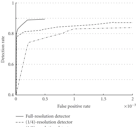
Figure16: Receiver operating characteristics for detectors at vary-ing integral image resolutions.

8. PEOPLE DETECTION RESULTS

Now we present the results of training the cascaded people detector using AdaBoost. We also give the results of evaluat-ing the accuracy of the trained detector on a test set.

8.1. Training the detector

We use 2252 people instances and the same number of non-people instances to train the first stage of the cascaded clas-sifier. Each subsequent stage is trained with the same 2252 people images and 2252 false positives of the previous stages collected from a set of 1500 frames. The number of cascade stages and the size of each stage (i.e., the number of local image features in each stage) are determined automatically with a validation set containing 1585 people instances and 2 901 421 nonpeople images. Because of on-chip memory re-strictions, we constrain the cascade construction to a maxi-mum of 5 stages with the maximaxi-mum sizes of (in layer order) 20, 50, 100, 250, and 500. These values are found empirically to be suﬃcient for constructing a reasonably accurate and fast classifier. The details of the cascade construction algo-rithm can be found in [2]. When using (1/4)-resolution level for approximating the integral image, the training algorithm generates a 5-stage cascade classifier with stage sizes 20, 50, 98, 205, and 310, for a total of 683 features.

8.2. Test results

To evaluate the accuracy of the trained detector, we test it on a set of frames containing 981 people instances and 1 246 644 nonpeople instances. (These instances are not used either for training or validation.) The receiver operating characteristic (ROC) of the detector on this test set is shown inFigure 16. For comparison, we also show the ROC for detectors trained on exact integral images and (1/8)-resolution approximate

3

2_.5

2

1.5

1

0.5

0

N

o

.o

f

sub

w

indo

w

s

seen

b

y

stage

×106

1 2 3 4 5

Cascade stage number

Full-resolution detector (1/4)-resolution detector (1/8)-resolution detector

Figure17: Number of subwindows seen by each stage of the cas-cade.

integral images. (Note that for each detector, the same res-olution is used in approximating the integral images during both training and testing.) Clearly, the ROC improves as the approximation error of the integral image decreases. So there is a tradeoﬀbetween the accuracy of the detector and the computational eﬀort needed for approximating the integral image.

It is also important to compare the average number of features computed per subwindow by each detector. This is because the computational savings obtained by approximat-ing the integral image may be lost if the approximation er-ror causes the detector to be computationally more expensive during detection. On the test set, the full-resolution detector computes 40.48 features per subwindow, the (1/4)-resolution detector computes 40.43 features per subwindow, while the (1/8)-resolution detector computes 47.94 features per sub-window. So the (1/4)-resolution and the full-resolution de-tectors require approximately the same amount of computa-tion during deteccomputa-tion. However, the (1/8)-resolucomputa-tion detec-tor needs more computations because the subwindows get past more of its cascade stages, as shown byFigure 17. There-fore, the savings provided by the (1/8)-resolution approxi-mate integral image are lost during the detection process.

(13)

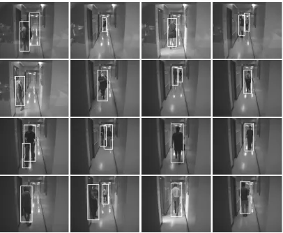
Figure18: Examples of frames scanned with the (1/4)-resolution detector.

subwindows can be classified easily, this strategy results in significantly more eﬃcient detection compared to using one large single-stage detector.

Figure 18shows examples of frames scanned using the (1/4)-resolution detector. Since the detector is insensitive to slight shifts and small size diﬀerences in a people instance, it almost always detects a single people instance multiple times during scanning. But many false positives tend to be isolated detections. So isolated detections are ignored and highly overlapping detections are averaged to obtain a single detection window.

9. FIRMWARE PERFORMANCE ANALYSIS

Given the primitive interfaces available for board-computer communications in the prototyping setup, extensive tests could not be performed on the physical implementation of this algorithm. However, a detailed analysis of the algorithms accuracy was extracted from the full software implementa-tion, as shown inSection 8. Given the functional equivalence between these two approaches, the analysis found therein should hold true for the hardware implementation as well. Exact timing numbers are equally diﬃcult to extract from the physical chip. However, synthesis tools are very proficient at estimating the internal delays with greater precision than

might even be achieved through direct measurement. Com-bining these estimates with functional models and extrapo-lating using the statistical distributions observed in the soft-ware implementation, it is possible to get an accurate mea-sure of what the system’s average performance should be un-der various circumstances.

(14)

estimate than using local measures. It is important to note that memory throughput could be further optimized by cus-tomizing the memory controller to take advantage of natural pauses in memory accesses to refresh or activate the memory banks in view of future accesses. This would have the eﬀect of lowering the average memory access time, thereby increasing the overall performance.

The creation and storage of the integral image to memory for a 352×288 image, cropped to 216×288 by the hardware, is approximately 30 milliseconds. This is governed by the number of points written to memory, which is fixed from one image to the next, and therefore should be relatively constant. Evaluation of the average frame rate of the detector is com-plicated by the fact that the number of points that need to be calculated varies according to the number of near-people windows in the image. Using a sample space of 981 frames containing people, it is found that on average, 40.43 features are required in each of the 3079 windows of an image. As-suming an average of 7 points per feature, this means that there are approximately 870 000 points evaluated in an av-erage frame. Given a memory access time hovering around 350 nanoseconds per point, it can be estimated that frames containing people can be treated at the rate of approximately 1 frame every 0.3 seconds. In comparison, treating an image that has very few false positives can take as little as 25 mil-liseconds once the integral image has been written to mem-ory.

Of course, this is assuming that the memory controller is able to run at 100 MHz. Although this should be possible, recent versions of the synthesis tools have unexpectedly been unable to meet the timing constraints at such speeds. This forces the use of the on-chip digital clock managers (DCM) to synthesize a slower clock. Although the DCMs allow syn-thesis of the most rational number multiples of the input clock, 75 MHz is sufficiently slow and reduces complications in crossing clock domains. With the design running at this speed, the frame rate with a subject in the image should drop from around 3 fps to slightly under 2.5 fps. This constraint makes running the design at full speed less of an issue. This turns out to be quite useful, as the synthesis tools were not quite able to meet the 10-nanoseconds period requirement, even by using the highest effort level for placement and rout-ing, due to some paths of excessive length in the MicroBlaze processor. While careful floorplanning should make it pos-sible to run the design at 100 MHz, the memory controller’s speed limitations make this not worth the effort, especially considering that it would be significantly more trouble.

Synthesizing the design without the MicroBlaze proces-sor (leaving only the framework’s ASFW) reveals that the 100 MHz constraint could be satisfied if the MicroBlaze were replaced by an oﬀ-chip processor. Given that the place and route tools abandon their search for greater performance once the requirements are met, it is possible that this design could run slightly faster still, but the trouble that the tools had in achieving even this level of performance hint that this would probably not be a significant gain. The fact that sys-tem performance is limited by memory bandwidth makes any possible speed optimizations unnecessary.

The place and route reports also show that the system has some space remaining for extra logic, with the design only taking up 3438, or 67%, of all slices in the Virtex-II 2V1000 chip. In fact, excluding the MicroBlaze, the full system only takes 2233, or 43%, of the available space. A more significant diﬀerence is in the usage of Block Select RAMs, and hard-ware multipliers. Although the ASFW only uses 7 blocks of memory and 9 multipliers, the MicroBlaze requires an extra 18 blocks of memory, and an extra 3 multipliers. This means that while the ASFW accounts for 65% of the logic used by the entire system, the MicroBlaze accounts for 72% of the memory used.

10. CONCLUSIONS AND FUTURE WORK

In this paper, we have designed an FPGA-based people detec-tion system based on the Viola-Jones object detecdetec-tion algo-rithm. We have introduced a novel algorithm for computing an approximate integral image from DCT coeﬃcients that is suitable for hardware implementation. Our work has ex-plored some of the hardware issues involved in implement-ing our system on FPGA. We have developed methods for adapting algorithms which make use of floating-point op-erations and which require access to large amounts of data. Dealing with such obstacles is a necessary step in adapting the more complex, and more interesting, computer vision algo-rithms to FPGAs. We have also shown that a relatively simple platform suitable for widespread, low-cost distribution into a network configuration can handle image processing tasks of moderate complexity with a low latency.

The current iteration of this project does not have a hard-ware training module. However, given that the FPGA-based detector will be operating on the same images as the soft-ware one, the training can be done in softsoft-ware and the results loaded into hardware. Since the training data is currently hardwired into the HDL code, it is necessary to resynthe-size the code whenever a new training set needs to be loaded. However, it is a relatively simple matter to isolate the parts of the bitstream that correspond to this data and modify them. This allows the creation of a partial reconfiguration bitstream which only modifies the memory locations containing train-ing data and leaves the rest of the FPGA untouched. In fact, it should be possible to use the MicroBlaze itself to reconfigure these sections using the Virtex-II’s internal configuration ac-cess port (ICAP). For memory segments that only ever need to be changed in their entirety, or that are seldom modified, partial reconfiguration of the memory segments permits the read/write capabilities of RAM without the added complex-ity of providing a datapath and control for writing to that memory.

(15)

data written by the trainer. The detector will then automati-cally be using the new training data, without the need to ex-plicitly load it. However, this requires a judicious use of hard macros in both modules, and may lead to suboptimal place-and-route in one or both modules. Since real-time training is not required, suboptimal performance in the trainer can be accepted, which suggests that the detector be optimized first, and the trainer be implemented according to the restrictions this imposes.

More immediate gains could be achieved through devel-opment of a caching module to reduce the need for external memory accesses, directly improving system performance. This is aided by the possibility of developing application cific cache architectures to take full advantage of a task’s spe-cific memory access patterns, thereby further taking advan-tage of the FPGA’s reconfigurability. However, whether or not individual nodes are working at peak eﬃciency, it is unfeasi-ble that large numbers of cameras in widely disparate envi-ronments could be hand trained. It would be preferable to have some method allowing unsupervised, automatic train-ing of the cameras; and so we come full circle to that which guided the design of the node’s architecture, which is the in-clusion of this module into a networked environment, work-ing hand in hand on more complex tasks that no module could tackle independently.

REFERENCES

[1] K. Nguyen, G. Yeung, S. Ghiasi, and M. Sarrafzadeh, “A gen-eral framework for tracking objects in a multi-camera envi-ronment,” inProc. 3rd International Workshop on Digital and Computational Video (DCV ’02), pp. 200–204, Clearwater, Fla, USA, November 2002.

[2] P. Viola and M. Jones, “Robust real-time object detection,” in2nd International Workshop on Statistical and Computa-tional Theories of Vision – Modeling, Learning, Computing, and Sampling, Vancouver, Canada, July 2001, www.stat.ucla.edu/ ∼sczhu/workshops/SCTV2001.html.

[3] E. Cerro-Prada, S. M. Charlwood, and P. B. James-Roxby, “Designing image processing applications using reconfig-urable computing,” in7th International Conference on Image Processing and Its Applications, vol. 1, pp. 450–454, Manch-ester, UK, July 1999.

[4] N. Srivastava, J. L. Trahan, R. Vaidyanathan, and S. Rai, “Adaptive image filtering using run-time reconfiguration,” in Proc. International Parallel and Distributed Processing Sympo-sium, pp. 180–186, Nice, France, April 2003.

[5] T. W. Fry and S. Hauck, “Hyperspectral image compres-sion on reconfigurable platforms,” in10th Annual IEEE Sym-posium on Field-Programmable Custom Computing Machines (FCCM ’02), pp. 251–260, Napa, Calif, USA, April 2002. [6] A. B. Abdelali, L. Boussaid, A. Mtibaa, and M. Abid,

“Run-time reconfiguration for real-“Run-time low-level image processing: architecture and algorithm architecture adequation (AAA),” inIEEE International Conference on Systems, Man and Cyber-netics, vol. 2, pp. 69–73, Hammamet, Tunisia, October 2002.

[7] M. R. Boschetti, A. M. S. Adario, I. S. Silva, and S. Bampi, “Techniques and mechanisms for dynamic reconfiguration in an image processor,” inProc. 15th Symposium on Integrated Circuits and Systems Design, pp. 177–182, Porto Alegre, Brazil, September 2002.

[8] Y. Freund and R. E. Schapire, “Experiments with a new boost-ing algorithm,” inProc. 13th International Conference on Ma-chine Learning, pp. 148–156, Bari, Italy, July 1996.

[9] J. Miano, Compressed Image File Formats: JPEG, PNG, GIF, XBM, BMP, ACM Press. Addison-Wesley Professional, Boston, Mass, USA, 1999.

[10] G. K. Wallace, “The JPEG still picture compression stan-dard,” IEEE Trans. Consumer Electron., vol. 38, no. 1, pp. 18– 34, 1992.

Vinod Nair received the B.Eng. degree in 2002 and the M.Eng. degree in electri-cal engineering in 2004, both from McGill University, Montreal, Canada. He is cur-rently pursuing his Ph.D. in computer sci-ence at the University of Toronto, Canada. His main research interests are in machine learning and computer vision.

Pierre-Olivier Laprisereceived the B.Eng. degree in computer engineering in 2001 and the M.Eng. degree in electrical engineering in 2004 from McGill University, Montreal, Qu´ebec, Canada. His Master’s research fo-cused on the application of reconfigurable-computing embedded systems to computer vision. He worked as a Research Assistant to Professor James J. Clark in the Motor Vi-sion Lab of the Centre for Intelligent

Ma-chines, McGill University, from September 2001 to June 2004. He was awarded a PRECARN Scholarship in 2002. He currently works as a Junior Product Design Engineer for PMC Sierra, Inc., Mon-treal, Qu´ebec, Canada.

James J. Clarkis a Professor in the Depart-ment of Electrical and Computer Engineer-ing, McGill University, Montreal, which he joined as an Associate Professor in 1996. He is currently an Associate Chairman (acting) of the department. From 1994 till 1996, he was a Visiting Researcher at Nissan Cam-bridge Basic Research, CamCam-bridge, Mas-sachusetts. From 1985 through 1994, he was a faculty member in the Division of Applied