Modified Clipped LMS Algorithm
Mojtaba Lotfizad
Department of Electrical Engineering, Tarbiat Modarres University, P.O. Box 14115-143, Tehran, Iran Email:[email protected]
Hadi Sadoghi Yazdi
Department of Electrical Engineering, Tarbiat Modarres University, P.O. Box 14115-143, Tehran, Iran Email:sadoghi [email protected]
Received 30 May 2004; Revised 22 January 2005; Recommended for Publication by Mark Kahrs
A new algorithm is proposed for updating the weights of an adaptive filter. The proposed algorithm is a modification of an existing method, namely, the clipped LMS, and uses a three-level quantization (+1, 0,−1) scheme that involves the threshold clipping of the input signals in the filter weight update formula. Mathematical analysis shows the convergence of the filter weights to the optimum Wiener filter weights. Also, it can be proved that the proposed modified clipped LMS (MCLMS) algorithm has better tracking than the LMS algorithm. In addition, this algorithm has reduced computational complexity relative to the unmodified one. By using a suitable threshold, it is possible to increase the tracking capability of the MCLMS algorithm compared to the LMS algorithm, but this causes slower convergence. Computer simulations confirm the mathematical analysis presented.
Keywords and phrases:adaptive filter, LMS algorithm, clipped LMS algorithm, modified clipped LMS algorithm.
1. INTRODUCTION
Adaptive signal processing has been one of the fastest grow-ing fields of research in recent years. It has attained its pop-ularity due to a broad range of useful applications in such diverse areas as communications, radar, sonar, seismology, navigation and control systems, and biomedical electronics. The LMS adaptive filter is very popular due to its simplic-ity, but even simpler approaches are required for many real-time applications, several different versions of the LMS algo-rithm have been proposed in the literature [1,2,3,4,5,6]. Reduction of the complexity of the LMS algorithm has re-ceived attention in the area of adaptive filters [5,7,8,9]. The sign algorithm and clipped data algorithm are in this cate-gory [2,5,8,9,10].
The tracking behavior of adaptive filtering algorithms is a fundamental issue in defining their performance in non-stationary operating environments. It has been established that adaptive algorithms that exhibit good convergence prop-erties in stationary environments do not necessarily provide good tracking performance in a nonstationary environment because the convergence behavior of an adaptive filter is a transient phenomenon, whereas the tracking behavior is a steady-state property [11,12]. Thus, much research is done for the measurement of tracking performance of variants of the LMS algorithm from different views [10,13,14,15].
For applications in which slow adaptation is acceptable, the clipped LMS (CLMS) algorithm has an edge over the
others in terms of speed of processing [16]. Also fast CLMS is proposed for increasing the speed of convergence [2].
Much effort from the viewpoint of reduction of the com-putations of the LMS algorithm is seen in the aforemen-tioned references. The present work concerns the presenta-tion of a modified version of the CLMS algorithm whose tracking is much better than the CLMS and LMS and has less computation as well.
The variants of LMS are discussed inSection 2. The pro-posed new algorithm, which is a modification of the afore-mentioned algorithm, appears inSection 3.Section 4deals with the computation of tracking performance of the pro-posed algorithm.Section 5is concerned with computer sim-ulation issues. Reduction of computational complexity of the proposed algorithm is investigated in Section 6. The final section presents conclusions for the present work and sum-marises the main findings.
2. VARIANTS OF THE LMS ALGORITHM
The purpose of this section is to briefly introduce the main existing variants of the LMS algorithm. In order to clarify the background of the new algorithm, it is necessary to show how they are interrelated and how they have evolved. The LMS algorithm has been studied in [17,18] as
sgn(x) 1
−1
x
Figure1: Quantization scheme for the clipped LMS algorithm.
where
en=dn−XnTWn, (2)
Wn=[wn(1),wn(2),. . .,wn(N)]T is the weight vector of the estimator,Xnis the vector of the input data sequence, which is assumed to be a stationary random process,Nis the num-ber of filter taps,enis the estimation error,dnis the desired response, andµis the step size.
A simple change can be made to the LMS algorithm to obtain the CLMS algorithm [2,16,19]:
Wn+1=Wn+µenXn, (3)
whereXis the clipped input signal vector, whoseith com-ponent is ˜x(i)=sgn[x(i)]. Other variations of the LMS algo-rithm that have been studied are the “sign” algoalgo-rithm [20,21]
Wn+1=Wn+µe˜nXn, (4)
where
˜
en=sgn
en
, (5)
and “the zero-forcing” algorithm [22,23]
Wn+1=Wn+µe˜nXn. (6)
The CLMS algorithm involves clipping the input signal vector in the weight update formula (3). This quantization scheme can best be illustrated byFigure 1.
3. THE PROPOSED MODIFIED CLIPPED LMS ALGORITHM
Here we propose a new modification to the clipped LMS al-gorithm to further simplify the implementation of the LMS algorithm. Rather than representing the input signal Xnby a two-level signal as shown earlier by (3), we quantize it into a three-level signal according to the quantization scheme shown in Figure 2. Thus, the adaptation equation can be written as
Wn+1=Wn+µenXn, (7)
msgn(x,δ) 1
−1
x δ
−δ
Figure2: Quantization scheme for the modified clipped LMS algo-rithm.
whereXnis the modified clipped input signal vector whose ith component isxn(i)= msgn[xn(i),δ], where msgn{·}is the modified sign function defined as
msgnxn(i),δ
=
+1, δ≤xn(i), 0, −δ < xn(i)< δ, −1, xn(i)≤ −δ.
(8)
It should be noted that the implementation of such an adaptive filter has potentially greater throughput because for those times when the tap input signal xn(i) is less than the specified threshold,δ, thenxn(i) will be equal to zero and no coefficient adaptation for the corresponding weight needs to be performed.
This means that some of the time-consuming operations in the weight update formula (7) can be omitted, thereby leading to a reduction of the computational load on the pro-cessor. Whether this potential can be realised depends on the architecture used in the processor and also the application. Convergence of the mean of the weight vector for MCLMS is proved in the next subsection. It is shown that the mean of the weight vector of the modified clipped LMS algorithm converges to the optimum weight vector of the Wiener filter.
3.1. Derivation of the convergence of the MCLMS algorithm
Now, we want to prove that the statistical average of the weight vector converges in the limit to the optimum Wiener weight vector. Taking expectations on both sides of (7) yields
EWn+1
=EWn
+µEenXn
. (9)
Substituting (2) in (10) gives
EWn+1
=EWn
+µEdnXn−XnXnTWn
. (10)
Assuming lack of correlation between the weights andXnXnT as in [17], (10) gives
EWn+1
=EWn
+µEdnXn
−E XnXnT
EWn
.
(11)
Now, with regard to (A.1) in the appendix, we have
EWn+1
=EWn
+µ
α σxP−
α σxRE
Wn
=
I−µα σxR
EWn
+µα
σxP ,
where α= 2 πexp
− δ2 2σ2
x
, (13)
andσxis the standard deviation of the input signal. We know that the optimum Wiener weight vector isW∗=R−1P.
Sub-stituting in (13) yields
EWn+1
=
I−µα σxR
EWn
+µα
σxRW
∗. (14)
IfVn=Wn−W∗, then
EVn+1
=
I−µα σxR
EVn
. (15)
Now, the principal axes are rotated according toV =QV, where the rows ofQare eigenvectors ofR=QΛQ−1andΛis
a diagonal matrix whose elements are eigenvalues ofR. Thus we have the following relation:
EQVn+1
=
I−µα
σxR
EQVn
, (16)
whereQandVkare uncorrelated becauseRandW are un-correlated. Thus,
EVn+1
=Q−1
I−µα
σxR
QEVn
=
Q−1IQ−µα σxQ
−1RQ
EVn
=
I−µα σxΛ
EVn
.
(17)
If (I−µ(α/σx)Λ)n in the limit converges to zero, then limn→∞E{Vn+1}=0. In this case, limn→∞E{Vn+1}=0 and
con-sequently limn→∞E{Wn+1} =W∗, that is, the MCLMS
algo-rithm will converge. In order that limn→∞(I−µ(α/σx)Λ)n= 0, it is necessary to find a condition for µin terms of the eigenvalues. We have
lim
n→∞
I−µα
σxΛ n = lim n→∞ 1−µα
σxλ0 n
· · · 0 ..
. . .. ...
0 lim
n→∞
1−µα
σxλN n
=0.
(18)
Therefore, the convergence condition is that for each eigen-value of matrix R,µsatisfies the following relation:
0< µ <α
σx 1
λi
, 1≤i≤N. (19)
Ifµsatisfies this relation for the largest eigenvalueλmax, then (19) is also satisfied for all other eigenvalues. Thus, the con-vergence condition for MCLMS is as follows:
0< µ <α σx
1
λmax. (20)
Also, the time constant for the exponential relaxation of the weight vector to its optimal value is
τMCLMS= 1
(α/σx)µλmax. (21)
4. EVALUATING THE TRACKING PERFORMANCE OF THE MCLMS ALGORITHM
Tracking is a steady-state phenomenon that is different from the convergence, which is a transient phenomenon. In gen-eral, convergence and tracking are two different properties. That is, if an algorithm has good convergence, its tracking ability is not necessarily fast and vice versa. In the tracking phase, a reasonable assumption is that the optimum weights vary according to a first-order Markov process [12], and the filter must track these weights. The following relation shows the variation of the filter’s optimum weights:
Wn∗+1=aWn∗+ωn, dn=Wn∗TXn+νn, (22)
wherea is a constant andωn is the process noise vector in thenth step, which has zero mean with correlation matrix
Φ, andνnis the measurement noise, which is assumed to be white Gaussian with zero mean and varianceσ2
ν.
4.1. The misadjustment criterion in MCLMS
According to [12], the algorithm misadjustment is usable as a criterion in tracking:
MMCLMS=E ωT
nXn
2
Eνn2
. (23)
The above relation shows that the weight misadjustment is related to the process noise power andXn. Now, we calcu-late the misadjustment (23) in which the numerator can be written as
EωT
nXn2
=EωT
nXnXkTωn
. (24)
With the assumption of independence ofXnandωnand us-ing relation (A.1) in the appendix,
EωTnXnXnTωn
=trEωnTXn
E XnTωn
=tr
α σxE
ωT
nXn
α
σxE
XT
nωn
= α σx 2
tr{RΦ}.
1000 900 800 700 600 500 400 300 200 100 0
Iteration number 10−20
10−15
10−10
10−5
100
105
W
eig
ht
er
ro
r
(dB)
LMS CLMS
MCLMS
Figure3: Weight estimation error, norm of the difference weight vector.
Also, the denominator of the fraction (23) is
Eνn2
=σ2
n. (26)
Hence, the MCLMS algorithm misadjustment can be written as
MMCLMS= 1 σ2
ν
α σx
2
trRΦ. (27)
Comparing this misadjustment value with that of the LMS algorithm, MLMS=(1/σν2) tr{RΦ}, the following relation can
be obtained:
MMCLMS=
α σx
2
MLMS. (28)
The above relation shows that increasing the thresholdδsuch thatαin less thanσxgives rise to a decrease in the misad-justment error relative to LMS in tracking, but with regard to (21), it causes the MCLMS to be slower in convergence. In the next section, this issue will be shown for identification of a filter and its tracking.
5. APPLICATION OF MCLMS IN THE IDENTIFICATION PROBLEM
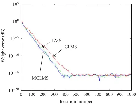
In order to demonstrate the convergence behavior of the LMS, CLMS, and the new MCLMS algorithm, 100 runs of simulation experiments have been performed (withµ=0.17 andδ =0.7 for MCLMS,µ=0.105 for LMS, andµ=0.13 for CLMS, which were the best parameters for maximum speed of convergence). In all experiments carried out for the system identification, a stationary white noise sequence was used and the system is a 7-tap FIR transversal filter having parameters that are arbitrarily chosen.
The input data were normalized to have unit variance. The norm of the difference between the plant FIR weights
0.9 0.85 0.8 0.75 0.7 0.6 0.5 0.4 0.3 0.2
Thresholdδ 0
5 10 15 20 25
R
el
at
iv
e
re
d
u
ct
io
ni
ne
rr
o
r
o
f
M
C
L
M
S
MCLMS/CLMS
MCLMS/LMS
Figure 4: Relative reduction in error of MCLMS compared with CLMS and LMS with step size of 0.1 for MCLMS and different thresholds with best step size for least tracking error for LMS and CLMS.
and adaptive filter weights generated by each algorithm was averaged over 100 independent simulation runs and plotted as a function of time, as depicted inFigure 3. The norm is calculated by
norm(h,W)= i
hi−Wi
21/2
. (29)
It can be seen that MCLMS has much better convergence than CLMS and it is also almost as good as LMS in terms of convergence speed.
Of course, the MCLMS speed of convergence is reduced by increasing the threshold δ. In the above case with a threshold of 0.7, the difference weight norm of CLMS is im-proved by 12%, whereas the CLMS in comparison to the LMS has both lower convergence speed and higher weight error.
Figure 4shows the ratio of tracking error norm for weights of the proposed MCLMS algorithm to optimum weights of LMS and CLMS. The existence of the second parameter in the MCLMS algorithm, that is,δ, in comparison with LMS and CLMS, has caused an increase in its performance.
6. REDUCTION OF COMPUTATIONAL COMPLEXITY OF THE MCLMS RELATIVE TO THE CLMS ALGORITHM
The proposed algorithm has less computational complexity relative to the CLMS algorithm. If we assume that the input signal has a Gaussian distribution with zero mean and stan-dard deviationσx, then the probability that the signal falls in the interval between [−δσx,δσx] is
P−δσx< x < δσx
= −δσx
−δσx
Nµx,σx
Table1: Rate of reduction of computational complexity in weight update for MCLMS in comparison to CLMS.
Thresholdδ 0.1 0.4 0.7 1.0
Percentage of computational reduction
7.97 31.09 51.61 68.27
whereN(µx,σx) is the input probability density function and P(−δσx < x < δσx) which, in addition to being the proba-bility of the occurrence of the signal in interval [−δσx,δσx], is also the computational reduction of MCLMS relative to CLMS. The reason is that the signal is falling between the two thresholds with a probability ofP(−δσx< x < δσx), and within this interval, the proposed algorithm has no weight update, since according to (8) msgn[xn(i),δσx] is equal to zero. The computational reduction of MCLMS compared to the CLMS is shown inTable 1for several different thresholds. It is interesting to note that regarding (30) andFigure 4
forδ=0.7, the computational complexity of the weight up-date formula can be reduced about 52% without any notice-able change in the convergence behavior.
7. CONCLUSIONS AND SUGGESTIONS FOR FURTHER WORK
A proposed modified clipped LMS algorithm for discrete-time adaptive FIR filtering has been studied. This new algo-rithm was analytically treated from a theoretical viewpoint and the convergence rate and tracking performance from a misadjustment viewpoint were derived. The advantages in-clude a simple weight update formula, better convergence capability, and better tracking performance. Further work could apply the three-level clipping idea to the error signal instead of the input signal.
APPENDIX
Theorem 1. If two random variables u and v both have a Gaussian distributionN(0,σu)andN(0,σv), respectively, and E{uv} =ρσuσv,v=msgn(v,δ), then
Euv= α
σvE{uv}
, (A.1)
whereα=√2/πexp(−δ2/2σ2
v).
Proof. We define the random variable
z= u
σu − ρ σvv.
(A.2)
Now we have
E{zv} =E
u σu−
ρ σvv
v
=E
u σuv
−E
ρ σvv
2
. (A.3)
With regard to the assumption of the theorem,
E{zv} = ρσuσv
σu − ρ σvσ
2
v=0. (A.4)
Therefore zandvare uncorrelated. Also, therefore, sincez
andvare uncorrelated, we haveEzv=E{z}Ev=E{z}× 0=0.
Ezv=E
u σu−
ρ σvv
v
=0=⇒ (A.5)
1
σuE
uv= ρ
σvE
vv=⇒Euv=ρσu σv E
vv. (A.6)
On the other hand,
vv=v×msgn(v,δ)= |v|
, |v|> δ,
0, |v| ≤δ. (A.7)
The density function ofvvis also Gaussian with distribution
N(0,σv) hence,
Evv= +∞
−∞|v| 1 √
2πexp
−v2 2σv
dv
=2 +∞
+δ |v| 1 √
2πexp
−v2 2σv
dv
(A.8)
=
2
πσvexp
−δ2 2σ2
v
. (A.9)
Now regarding (A.6) and (A.9) we have
Euv=ρσu
σv
2
πσvexp
−δ2 2σ2
v
= 1
σv
2
πexp
−δ2 2σ2
v
ρσuσv.
(A.10)
Finally, with regard to E{uv} = ρσuσv in (A.10), we have proved the theorem.
ACKNOWLEDGMENT
The authors wish to thanks an anonymous reviewer for his/her helpful comments.
REFERENCES
[1] E. Ferrara, “Fast implementations of LMS adaptive filters,” in
IEEE Transactions on Acoustics, Speech, and Signal Processing, vol. 28, pp. 474–475, 1980.
[2] L. Deivasigamani, “A fast clipped-data LMS algorithm,” in
IEEE Transactions on Acoustics, Speech, and Signal Processing, vol. 30, pp. 648–649, 1982.
[3] J. A. Chambers, O. Tanrinkulu, and A. G. Constantinides, “Least mean mixed-norm adaptive filtering,” Electronic Let-ter, vol. 30, no. 19, pp. 1574–1575, 1994.
[5] C. Kwong, “Dual sign algorithm for adaptive filtering,” IEEE Trans. Commun., vol. 34, no. 12, pp. 1272–1275, 1986. [6] A. Ahlen, L. Lindbom, and M. Sternad, “Analysis of
sta-bility and performance of adaptation algorithms with time-invariant gains,” IEEE Trans. Signal Processing, vol. 52, no. 1, pp. 103–116, 2004.
[7] E. Eweda, “Analysis and design of a signed regressor LMS algorithm for stationary and nonstationary adaptive filtering with correlated Gaussian data,”IEEE Transactions on Circuits and Systems, vol. 37, no. 11, pp. 1367–1374, 1990.
[8] W. A. Sethares, I. M. Y. Mareels, B. D. O. Anderson, C. R. John-son Jr., and R.R. Bitmead, “Excitation conditions for signed regressor least mean squares adaptation,” IEEE Transactions on Circuits and Systems, vol. 35, no. 6, pp. 613–624, 1988. [9] V. Mathews and S. Cho, “Improved convergence analysis of
stochastic gradient adaptive filters using the sign algorithm,” inIEEE Transactions on Acoustics, Speech, and Signal Process-ing, vol. 35, pp. 450–454, 1987.
[10] E. Eweda, “Comparison of RLS, LMS, and sign algorithms for tracking randomly time-varying channels,”IEEE Trans. Signal Processing, vol. 42, no. 11, pp. 2937–2944, 1994.
[11] P. C. Wei, J. Han, J. R. Zeidler, and W. H. Ku, “Compara-tive tracking performance of the LMS and RLS algorithms for chirped narrowband signal recovery,”IEEE Trans. Signal Pro-cessing, vol. 50, no. 7, pp. 1602–1609, 2002.
[12] S. Haykin, Adaptive Filter Theory, Prentice-Hall, Englewood Cliffs, NJ, USA, 3rd edition, 1996.
[13] M. Hajivandi and W. A. Gardner, “Measures of tracking per-formance for the LMS algorithm,” inIEEE Transactions on Acoustics, Speech, and Signal Processing, vol. 38, pp. 1953– 1958, 1990.
[14] B. Farhang-Boroujeny and S. Gazor, “Performance of LMS-based adaptive filters in tracking a time-varying plant,”IEEE Trans. Signal Processing, vol. 44, no. 11, pp. 2868–2871, 1996. [15] L. Lindbom, M. Sternad, and A. Ahlen, “Tracking of
time-varying mobile radio channels—part 1. The wiener LMS algo-rithm,”IEEE Trans. Commun., vol. 49, no. 12, pp. 2207–2217, 2001.
[16] M. White, I. Mack, G. Borsuk, D. Lampe, and F. Kub, “Charge-coupled device (CCD) adaptive discrete analog signal process-ing,”IEEE Trans. Commun., vol. 27, no. 2, pp. 390–405, 1979. [17] B. Widrow and S. Stearns, Adaptive Signal Processing,
Prentice-Hall, Englewood Cliffs, NJ, USA, 1985.
[18] B. Farhang-Boroujeny, Adaptive Filters, Theory and Applica-tions, John Wiley & Sons, West Sussex, England, 1999. [19] J. L. Moschner, Adaptive filtering with clipped input data,
Ph.d.thesis, Stanford University, Stanford, Calif, USA, June 1970.
[20] N. Verhoeckx, H. van den Elzen, F. Snijders, and P. van Ger-wen, “Digital echo cancellation for baseband data transmis-sion,” IEEE Trans. Signal Processing, vol. 27, no. 6, pp. 768– 781, 1979.
[21] T. Claasen and W. Mecklenbrauker, “Comparison of the con-vergence of two algorithms for adaptive FIR digital filters,”
IEEE Transactions on Circuits and Systems, vol. 28, no. 6, pp. 510–518, 1981.
[22] R. W. Lucky, “Automatic equalization for digital communica-tion,”Bell Syst. Tech. J., vol. 4, no. 4, pp. 547–588, April 1965. [23] B.-E. Jun, D.-J. Park, and Y.-W. Kim, “Convergence analysis of sign-sign LMS algorithm for adaptive filters with correlated Gaussian data,” inIEEE International Conference on Acoustics, Speech, and Signal Processing (ICASSP ’95), vol. 2, pp. 1380– 1383, Detroit, Mich, USA, May 1995.
Mojtaba Lotfizadwas born in Tehran, Iran, in 1955. He received the B.S. degree in elec-trical engineering from Amir Kabir Univer-sity, Iran, in 1980, and the M.S. and Ph.D. degrees from the University of Wales, UK, in 1985 and 1988, respectively. He then joined the Engineering Faculty Tarbiat Modarres University, Iran. He has also been a Con-sultant to several industrial and government organizations. His current research interests
are signal processing, adaptive filtering, speech processing, and spe-cialized processors.