R E S E A R C H
Open Access
Statistical covariance-matching based blind
channel estimation for zero-padding
MIMO–OFDM systems
Yi-Sheng Chen
1*and Jwo-Yuh Wu
2Abstract
We propose a statistical covariance-matching based blind channel estimation scheme for zero-padding (ZP) multiple-input multiple-output (MIMO)–orthogonal frequency division multiplexing (OFDM) systems. By exploiting the block Toeplitz channel matrix structure, it is shown that the linear equations relating the entries of the received covariance matrix and the outer product of the MIMO channel matrix taps can be rearranged into a set of decoupled groups. The decoupled nature reduces computations, and more importantly guarantees unique recovery of the channel matrix outer product under a quite mild condition. Then the channel impulse response matrix is identified, up to a Hermitian matrix ambiguity, through an eigen-decomposition of the outer product matrix. Simulation results are used to evidence the advantages of the proposed method over a recently reported subspace algorithm applicable to the ZP-based MIMO–OFDM scheme.
Keywords: Blind channel estimation, Zero padding, MIMO–OFDM
1 Introduction
Orthogonal frequency division multiplexing (OFDM) combined with guard intervals, in the form of cyclic pre-fix (CP) or zero-padding (ZP), is an effective transmission scheme through frequency selective fading channels [1]. By further leveraging the spatial resource, the multiple-input multiple-output (MIMO)–OFDM system has been the key technique for realizing high-rate transmission in modern wireless communications [2]. Toward reliable coherent symbol decoding in MIMO–OFDM systems, accurate channel state information is crucial. Blind chan-nel estimation is a technique that alleviates the need for training sequences to identify the unknown chan-nel impulse response from the received signal. Since the requirement of extra bandwidth for training overhead is reduced, this technique has received great research inter-est [3] and many blind inter-estimation algorithms have been developed for various transmission systems [3-21]. In this article, we will focus on blind estimation of ZP-based MIMO–OFDM systems.
*Correspondence: [email protected] 1Feng Chia University, Taichung, Taiwan
Full list of author information is available at the end of the article
For ZP-based single-input single-output (SISO) OFDM systems, a subspace algorithm is proposed to blindly iden-tify the channels in [20], and is then generalized to MIMO cases [21]. However, this approach is known to suffer a sever performance degradation when the signal-to-noise ratio (SNR) is low or moderate [5]. To solve this problem, a statistical covariance-matching (SCM) based method which exploits some priori knowledge of the signal struc-ture to improve channel estimation/equalization perfor-mances against harsh SNR conditions, is developed for SISO cases [6]. In this article we will propose an SCM based blind channel estimation for ZP-based MIMO– OFDM systems. By exploiting the block Toeplitz channel matrix structure, we show that the linear equations relat-ing the entries of the received covariance matrix and the products of the channel matrix taps can be rear-ranged into decoupled groups. The outer product of the MIMO channel matrices can be obtained by solving these decoupled linear equation groups. The channel impulse response is then identified, up to a Hermitian matrix ambiguity, through an eigen-decompostion of the com-puted outer product matrix. The proposed approach has the following distinctive features: (i) The identifiability condition is very simple and is more relaxed than the
irreducible or column reduced condition [8]; (ii) It can apply to the more transmit antennae case under a certain condition; (iii) Through numerical simulation, it yields improved BER performance in the low-to-moderate SNR region. The rest of this article is organized as follows. Section 2 is the system model and basic assumptions. In Section 3, we propose a blind channel estimation method for the ZP based MIMO–OFDM systems. Simulation results are given in Section 4. Section 5 concludes this article.
Notations used in this article are quite standard: Bold uppercase is used for matrices, and bold lowercase is used for vectors. AT represents transpose of the matrix A, and A∗ represents conjugate transpose of the matrix A. IM is the identity matrix of dimensionM×M, and A⊗B is the Kronecker product of matrices A and B. In addition, we define the following operations that will be used in the derivation of the main result. First, for any m×m matrixA =[ak,l]0≤k,l≤m−1, define j(A) = [a0,ja1,j+1. . .am−1−j,m−1]T for 0≤ j≤m−1, i.e.,j(A) is the vector formed from the jth super-diagonal of A. Second, for anyJn×JnmatrixB=[Bk,l]0≤k,l≤n−1, where Bk,lis a block matrix of dimensionJ×J, defineϒj(B) = [BT0,jBT1,j+1. . .BTn−1−j,n−1]Tfor 0≤j≤n−1, i.e.,ϒj(B)is the matrix formed from thejthblock super-diagonal ofB.
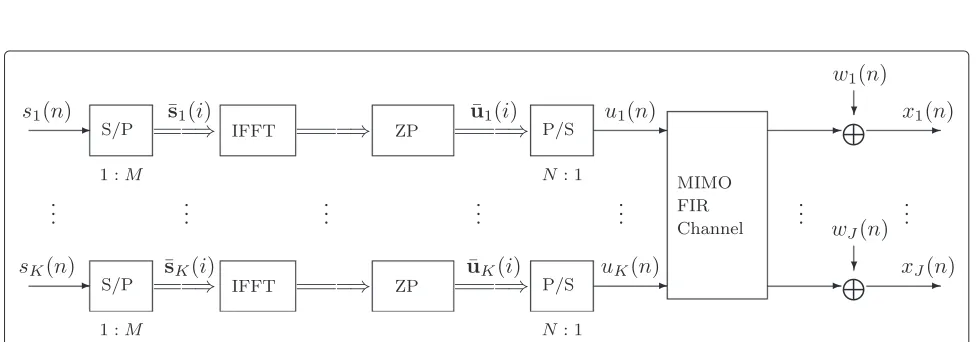
2 System model and basic assumptions
Consider the K-input J-output discrete time ZP-OFDM baseband model shown in Figure 1. At the transmitter, for k=1, 2,. . .,K, each input signal sk(n) is stacked as a block s¯k(i) = [sk(iM)sk(iM+1) . . .sk(iM+M−1)]T ∈ CM, which is multiplied by the inverse FFT matrixF∗, and then padded with P trailing zero entries to form the N=M + P
dimensional vector u¯k(i) =
⎡
⎣( F∗¯sk(i))T Mentries
0. . .0
Pentries
⎤ ⎦
T
=
⎡
⎣uk(iN) . . .uk(iN+M−1) Mentries
0. . .0
Pentries
⎤ ⎦
T
. The zero-padded
¯
uk(i)is parallel-to-serial converted to obtainuk(n), which is then transmitted through the MIMO finite-impulse-response (FIR) channel. At the receiver, thejth received signal isxj(n) = Kk=1
Ljk
l=0hjk(l)uk(n−l)+wj(n)for j=1, 2,. . .,J, wherewj(n)is the channel noise seen at the jth receiver, and {hjk(0)hjk(1) . . .hjk(Ljk)} is the impulse response from thekth transmitter to thejth receiver.
Let x(n) =[x1(n)x2(n) . . .xJ(n)]T∈ CJ, w(n) = [w1(n)w2(n) . . .wJ(n)]T∈CJ, andH(l) =[hjk(l)]∈CJ×K be the channel coefficient matrix for l = 0, 1,. . .,L, where L = maxj,k{Ljk}is the order of the MIMO chan-nel. Assume P ≥ L and group the sequence of x(n) as
¯
x(i) =[x(iN)Tx(iN +1)T. . .x(iN +N −1)T]T∈ CJN. Then due to zero padding, the input-output channel char-acteristics can be expressed in the following form [21]:
¯
x(i)=Hfuf(i)+ ¯w(i), (2.1)
where w¯(i) ∈ CJN is similarly defined as x¯(i), and Hf ∈ CJN×KM is a block Toeplitz matrix with [H(0)TH(1)T. . .H(L)T0. . .0]T∈ CJN×K being its first block column and [H(0)0. . .0]∈ CJ×KM being its first block row. uf(i) =[u(iN)Tu(iN + 1)T. . .u(iN + M− 1)T]T∈ CKMwithu(n) ∈ CK being similarly defined as x(n).
The problem we study in this article is blind estimation of the MIMO channel matrix tapsH(m), 0 ≤ m ≤ L, by using second-order statistics of the received data. The following assumptions hold throughout the article.
(A) The source signals(n)=[s1(n)s2(n) . . .sK(n)]T∈CK
is a zero mean white sequence withE[s(m)s(n)∗]=
δ(m−n)IK, whereδ(·)is the Kronecker delta function.
The noise is white zero mean withE[w(m)w(n)∗]=
δ(m − n)σw2IJ. In addition, the source signal is
uncorrelated with the noisew(n), i.e.,E[s(m)w(n)∗]= 0K×J,∀m,n.
(B) The concatenated channel impulse response matrix H =[H(0)TH(1)T. . .H(L)T]T∈ CJ(L+1)×K is full
column rank, i.e.,rank(H)=K.
3 Blind channel estimation
We first introduce the proposed method, assuming the noise is absent in Section 3.1; the case when noise is present and some distinctive features regarding the pro-posed method are discussed in Section 3.2.
3.1 Proposed approach: noiseless case
When noise is absent, (2.1) can be expressed asx¯(i) = Hfuf(i). By further defining the block source signal sf(i)=[s(iM)Ts(iM+1)T. . .s(iM+M−1)T]T∈CKM, we haveuf(i)=(F∗⊗IK)sf(i)[9], which is a zero mean vec-tor withE[uf(i)uf(i)∗]=(F∗⊗IK)(F∗⊗IK)∗=(F∗F)⊗ (IKIK) = IKMaccording to assumption(A). Then taking expectation ofx¯(i)x¯(i)∗, we get
Rf =E[x¯(i)x¯(i)∗]=HfH∗f. (3.1)
LetJ ∈ RN×N be a circulant matrix with the first row equal to [ 00. . .01]∈ R1×N andS =[IN−L0(N−L)×L]T∈ RN×(N−L). Then the block Toeplitz structure ofH
f allows us to writeHf =
L
k=0(JkS)⊗H(k), and hence
Rf =
L
k=0
(JkS)⊗H(k) L
l=0
(JlS)⊗H(l)
∗
= L k=0
L
l=0
(JkS)⊗H(k) (ST(JT)l)⊗H(l)∗
= L k=0
L
l=0
JkSST(JT)l⊗(H(k)H(l)∗).
(3.2)
The following proposition, whose proof is given in Appendix 1, shows that the matrixJkSST(JT)lhas special structures that allows for the decomposition of (3.2) into a group of decoupled equations.
Proposition 3.1: Let 0≤k,l ≤Lbe two non-negative integers. Forl=k+j, where 0≤j≤L−k, the upper tri-angular part ofJkSST(JT)lis zero with only thejth upper diagonal nonzero and is given by
j
JkSST(JT)l
=qk(1 :N−j, 1)∈RN−j, (3.3)
where qk = Jkq0, 0 ≤ k ≤ L − j, and q0 = [ 11 . . .1
(N−L)entries 00. . .0
L entries
]T∈RN.
Sinceϒj
JkSST(JT)l⊗(H(k)H(l)∗)=j
JkSST(JT)l ⊗H(k)H(l)∗, it follows from (3.2) and (3.3) that for 0≤j≤L,ϒj
Rf
can be described as follows:
ϒjRf
=ϒj
HfH∗f
= L
k=0 L
l=0 ϒj
JkSST(JT)l
⊗H(k)H(l)∗
= L
k=0 L
l=0 j
JkSST(JT)l
⊗H(k)H(l)∗
= L−j
k=0
qk(1 :N−j, 1)⊗H(k)H(k+j)∗
= L−j
k=0
qk(1 :N−j, 1)⊗IJ
H(k)H(k+j)∗
=MjFj,
(3.4)
whereFj =[(H(0)H(j)∗)T(H(1)H(j+1)∗)T. . . (H(L−j) H(L)∗)T]T∈ CJ(L−j+1)×J is formed from the products of channel matrix taps of the form H(k)H(k + j)∗, andMj =[q0(1 : N − j, 1)q1(1 : N −j, 1) . . .qL−j(1 : N−j, 1)]⊗IJ ∈RJ(N−j)×J(L−j+1).
SinceN > L+1, the (L+1) equations in (3.4) are overdetermined and consistent. Since it can be checked that Mj is full column rank for j = 0, 1,. . .,L (see Appendix 2), the solutionFjcan be obtained as
Fj=(MTj Mj)−1MTj ϒj
Rf
, j=0, 1,. . .,L. (3.5)
LetQbe the Hermitian matrix defined by Q = HH∗. Then we obtain Qfrom (3.5) since Qis Hermitian and ϒj(Q) = Fj forj = 0, 1,. . .,L. Since rank(H) = K by assumption(B),Qhas rankK. SinceQis Hermitian and positive semidefinite, QhasK positive eigenvalues, say, λ1,. . .,λK. We can expandQas
Q=
K
j=1
λjdj λjdj
∗
, (3.6)
wheredjis a unit norm eigenvector ofQassociated with λj>0. We can thus choose the channel impulse response matrix to be
H=[λ1d1
λ2d2 . . .
λKdK]∈CJ(L+1)×K. (3.7)
We note H can only be identified up to a unitary matrix ambiguity U ∈ CK×K [8], i.e., H = HU, since
3.2 Discussions
(1) The noisy case: When noise is present, the received
covariance matrix becomesRf =HfH∗f+σw2IJNbased
on (2.1). Since the matrixHf ∈CJN×KMis of full
col-umn rank, the rank ofHfH∗f isKM. This implies that
the assoicated smallest(JN−KM)eigenvalues ofRf
are equal to the noise variancesσw2. Hence, in
prac-tice we can obtain the estimated noise varianceσˆw2as
the average of the smallest(JN−KM)eigenvalues of
the sample covariance matrixRf. Then the proposed
channel estimation algorithm can directly apply by
substractingσˆw2IJNfromRf. Alternatively,σw2IJN can
also be estimated via the method given in [7]. (2) Channel identifiability: For the proposed method, the
channel identifiability condition is assumption (B),
i.e., rank(H) = K. Hence the channel needs not be
irreducible, column reduced [8], or full column rank
of H(0) required in the subspace method ([21], p.
1422). Thus the channel identifiability of the proposed method is more relaxed than that of the subspace method.
(3) Application to the more-input case: A necessary
con-dition for the concatenated channel matrixHto be of
full column rank (assumption(B)) is
J(L+1)≥K, (3.8)
i.e., the product of the number of receive antennae(J)
and the channel length(L+1)should be no less than
the number of transmit antennae(K). Hence, unlike
the subspace method [21], which is exclusive for the more-output case, the proposed method is also
capa-ble of identifying more-input channels (K > J), as
long as the condition (3.8) is fulfilled.
(4) Computational complexity: Compared with the sub-space method [21], the proposed method requires fewer computations. Detailed flop counts for these two methods are given in Appendix 3.
(5) Algorithm: We now summarize the proposed approach as the following algorithm:
(1) Collect the received data as x¯(i), and then
estimate the covariance matrixRf via the
fol-lowing time average
Rf = 1 S
S
i=1 ¯
x(i)x¯(i)∗, (3.9)
whereS is the number of symbol blocks.
(2) Use the method given in this subsection to
eliminate the noise componentσˆw2IJN
impos-ing onRf to getRc=Rf − ˆσw2IJN.
(3) Form the matrix Mj and compute Fj using
(3.5) for j = 0, 1,. . .,L. (Here we use Rc
instead ofRf in (3.5).)
(4) Form the matrixQusingF0,F1,. . .,FL, and
obtain the channel impulse response matrix
(3.7) by computing theK largest eigenvalues
and the associated eigenvectors ofQ.
4 Simulation
In this section, we use several numerical simulations to demonstrate the performance of the proposed method. We first consider two 2-input 2-output test channels, both withL=2. Channel A is shown as follows:
H(0)=
0.36+0.21j 0.48+0.29j
0.26+0.16j 0.5+0.17j
,
H(1)=
−0.49−0.36j 0.93+0.06j 0.88+1.30j 0.87+0.68j
,
H(2)=
0.73−0.14j −0.13−0.27j
0.29−0.4j −0.44−0.55j
,
and channel B is the same as channel A exceptH(0) =
0.48+0.24j 0.32+0.12j 0.24+0.13j 0.18+0.06j
. The length of symbol blocks
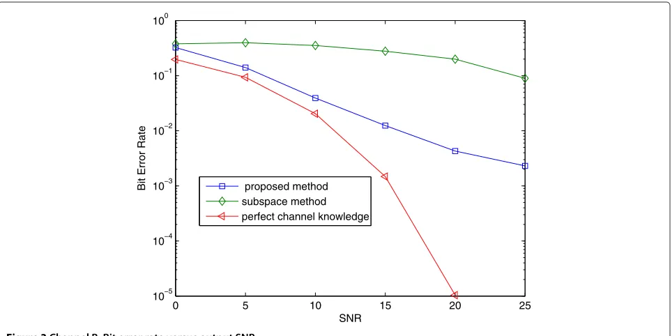
isM=18, which is zero padded to blocks of lengthM+ P =20. It meansP =2(=L)and transmission efficiency is 90%. The number of symbol blocks isS = 100. The channel normalized mean-square error (NMSE) is defined as NMSE = (1/I)Ii=1H(i)−H2F· H−F2, whereI = 200 is the number of Monte Carlo runs, and · Fdenotes the Frobenius norm. H(i) =[H(i)(0)TH(i)(1)TH(i)(2)T]T is theith estimate of the channel impulse response matrix H after removing the unitary matrix ambiguity by the least squares method [8]. The input source symbols are i.i.d. QPSK signals. The SNR at the output is defined as
SNR = E[x(n)−w(n)22] E[w(n)2
2]
. The channel noise is zero mean, temporally and spatially white Gaussian.
0 5 10 15 20 25 10−6
10−5 10−4 10−3 10−2 10−1 100
SNR
Bit Error Rate
proposed method subspace method perfect channel knowledge
Figure 2Channel A: Bit error rate versus output SNR.
channel A(=12.69), which means H(0) for channel B is closer to singularity (rank deficiency) and tends to violate the identifiability condition of the subspace method ([21], p. 1422).
In the second experiment, we generate 100 3-input 2-output random channels withL=2 to illustrate the esti-mation performance of the proposed method for channels with more transmitters than receivers. We useM = 18
andP=2. Each channel coefficient in the channel matrix is generated according to the independent complexed-valued Gaussian distribution with zero mean and unit variance. Figure 4 shows that for different numbers of symbol blocks, the proposed method is capable of iden-tifying the more-input channels. In addition, the NMSE decreases as SNR increases and is roughtly constant for high SNR. A possible explanation is that for sufficiently
0 5 10 15 20 25
10−5 10−4 10−3 10−2 10−1 100
SNR
Bit Error Rate proposed method subspace method perfect channel knowledge
0 5 10 15 20 25 30 −22
−20 −18 −16 −14 −12 −10 −8 −6
SNR
Channel NMSE(dB)
100 blocks 300 blocks 500 blocks
Figure 4Channel NMSE versus SNR (more-input channel case).
high SNR, the channel NMSE is contributed mainly due to numerical error than by channel noise. The existence of the error floor at high SNR due to numerical error is a well-known result, and this common phenomenon can also be observed in some previous works related to blind channel estimation [9-14].
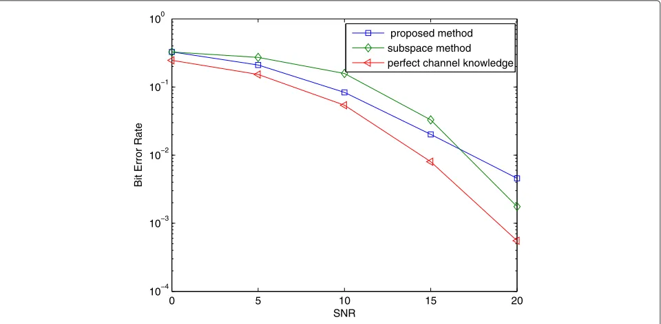
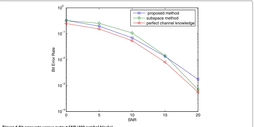
In the third experiment, we apply the proposed method to 200 2-input 4-out random channels with L = 4 to
demonstrate the performance. We useM = 36 andP = 4 to maintain the transmission efficiency at 90%. Each channel coefficient in the channel matrix is still generated according to the independent complexed-valued Gaussian distribution with zero mean and unit variance. Figures 5 and 6 show that as the number of symbol blocks (used to obtain the covariance matrixRf) increases from 200 to 400, the BER approaches to the ideal case. In addition,
0 5 10 15 20
10−4 10−3 10−2 10−1 100
SNR
Bit Error Rate
proposed method subspace method perfect channel knowledge
0 5 10 15 20 10−4
10−3 10−2 10−1 100
SNR
Bit Error Rate
proposed method subspace method perfect channel knowledge
Figure 6Bit error rate versus output SNR (400 symbol blocks).
these two figures also show that the proposed method out-performs the subspace method from low to medium SNR, and the subspace method performs better for high SNR.
In the literature of blind channel estimation, it is well-known that subspace methods, such as [18,21], enjoy the so-called “finite sample convergence” property [15-19,21], that is, in the noiseless case (or sufficicently high SNR), the channels can be almost exactly identified by using a finite number of samples for covariance estimation. This is the reason why the subspace-based solution can yield improved channel estimation accuracy and the resultant BER in the high SNR region. The proposed method, like most of other solution branches, e.g., [9-14], can be classified as the “SCM” approach, by which exact channel identification is achieved whenever the exact covariance matrix is available. Hence, it is not unexpected that our method is susceptible to finite-sample errors in covariance matrix estimation, which leads to an MSE floor in the high SNR region. Such a phenomenon is not uncommon in the literature, and has been seen in many studies, e.g., [9-14]. Despite this, the proposed method can outperform the subspace algorithm in the low SNR region, and hence could be a potential candidate in harsh communication environments.
5 Conclusion
We propose an SCM based blind channel estimation method for zero padding MIMO–OFDM systems. By exploiting the block Toeplitz channel matrix structure, we solve the channel product matrices from a series of
decoupled linear equations obtained from the covari-ance matrix of the received data. Then the channel impulse response matrix can be obtained by taking eigen-decomposition of a Hermitian matrix formed from the channel product matrices. The identifiability condi-tion is more relaxed than that of the subspace method [21]. Unlike most of existing solutions that are only applicable for the more-output channels, the proposed approach can also identify the more-input channels under a quite mild condition. Simulation results are used to demonstrate the performance of the proposed method. Compared with the subspace method [21], the pro-posed method is shown to have better performance form low to medium SNR or when H(0) tends to be singular.
Appendix 1: Proof of Proposition 3.1
Letenbe thenth column of the identity matrixIN. Then fork=0 case,
jJ0SS2(JT)j =j
[e1e2. . .eN−L0. . .0](JT)j
=
⎧ ⎪ ⎪ ⎪ ⎪ ⎨ ⎪ ⎪ ⎪ ⎪ ⎩
0([e1e2. . .eN−L0. . .0])=q0
j
⎛ ⎝ ⎡ ⎣0 . . .0
jcolumns
e1e2. . .eN−jeN−j+1. . .eN−L0. . .0
⎤ ⎦ ⎞ ⎠
=q0(1 :N−j, 1), 1≤j≤L.
Fork=1 case,
jJ1SST(JT)1+j =j
J[e1e2. . .eN−L0. . .0](JT)1+j
=j
[e2e3. . .eN−L+10. . .0](JT)1+j
= ⎧ ⎪ ⎪ ⎪ ⎪ ⎪ ⎨ ⎪ ⎪ ⎪ ⎪ ⎪ ⎩
0([0e2e3. . .eN−L+10. . .0])=Jq0=q1
j
⎛ ⎝ ⎡ ⎣0 . . .0
jcolumns
0e2e3. . .eN−L+10. . .0
⎤ ⎦ ⎞ ⎠
=q1(1 :N−j, 1), 1≤j≤L−1.
Hencej(J1G2(JT)1+j)=q1(1 :N−j, 1)for 0≤j≤L. Following the same process, we can obtain the cases j(JkG2(JT)k+j) = qk(1 : N −j, 1) fork = 2, 3,. . .,L, through some straightforward manipulation, and assert the result given in Proposition 3.1.
Appendix 2: Proof of full column rank ofMj
Let Pj =[q0(1 : N −j, 1)q1(1 : N − j, 1) . . .qL−j(1 : N−j, 1)]∈R(N−j)×(L−j+1)forj=0, 1,. . .,L. We note that P0is a Toeplitz matrix withq0being its first column and [ 100. . .0]∈R1×(L+1)being its first row. HenceP
0is full column rank.
Also we observe that forj = 1, 2,. . .,L,Pj is obtained fromP0by deleting its lastjrows and the lastjcolumns, i.e.,Pjis a Toeplitz matrix withq0(1 : N−j, 1)being its
first column and
⎡
⎣1 00 . . .0 L−j
⎤
⎦∈R1×(L−j+1)being its first row. Thus, forj=1, 2,. . .,L,Pjis full column rank.
SincePjis full column rank,Mj=Pj⊗IJ is full column rank forj=0, 1,. . .,L.
Appendix 3: Complexity evaluation
The proposed method is compared with the subspace method [21] in terms of flops, where a “flop” is defined to be a single complex multiplication or addition [22].
Proposed method: Estimate the (Hermitian) covariance matrixRf using (3.9); this requires(2S−1)JN(JN2+1) +1 flops. Estimate and eliminate the noise variance to obtain Rcneeds 3JNflops. Solving(L+1)least square problems using QR factorization ([22], p. 254) requires 2J3L
j=0(L− j+1)2[N −j− L−3j+1] flops. Eigen-decomposition of a J(L+1)×J(L+1)requires 12J3(L+1)3flops.
Subspace method: Estimate the covariance matrix
requires(2S−1)JN(JN2+1)+1 flops. Eigen-decomposition of a J(L + M) × J(L + M) matrix requires 12J3(L + M)3 flops. Singular value decomposition of a (JN − KM)N × J(L+ 1) matrix ([22], p. 240) requires 4J2(L+1)2[J(2L+2+N2)−KMN] flops.
According to the above flop computation, for the first experiment simulation in Section 4, the proposed method and the subspace method require about 1.7×10⁵ flops and 9.44×10⁵flops, respectively. For experiment 3 using 200 symbol blocks, the proposed method and the sub-space method require about 5.5×10⁶flops and 5.99×10⁷ flops, respectively.
Competing interests
The authors declare that they have no competing interests.
Acknowledgements
The research was sponsored by the National Science Council of Taiwan under grant NSC 99-2221-E-035-056-.
Author details
1Feng Chia University, Taichung, Taiwan.2National Chiao Tung University,
Hsinchu, Taiwan.
Received: 29 October 2011 Accepted: 6 June 2012 Published: 12 July 2012
References
1. Z Wang, GB Giannakis, Wireless multicarrier communications: where Fourier meets Shannon. IEEE Signal Process. Mag.17(3), 29–48 (2000) 2. GL St ¨uber, JR Barry, SW Mclaughlin, Y Li, MA Ingram, TG Pratt, Broadband
MIMO–OFDM wireless communications. Proc. IEEE.92(2), 271–294 (2004) 3. GB Giannakis, Y Hua, P Stoica, L Tong,Signal Processing, Advances in Wireless and Mobile Communications Volume I: Trends in Channel Identification and Equalization(Prentice Hall, PTR, Upper Saddle River, 2001)
4. YS Chen, CA Lin, Blind-channel identification for MIMO single-carrier zero-padding block-transmission systems. IEEE Trans. Circ. Syst.–I: Regular Papers.55(6), 1571–1579 (2008)
5. X Zhuang, Z Ding, AL Swindlehurst, A statistical subspace method for blind channel identification in OFDM communications. inProc. IEEE Int. Conf. Acoust. Speech Signal Process,5,(Philadelphia, Pennsylvania, USA, 2005), pp. 2493–2496
6. FD Backx, TTV Vinhozaand, R Sampaio-Neto, Blind channel estimation for zero-padded OFDM systems based on correlation matching. inProc. IEEE Vehicular Technology Conference – Fall,(Baltimore, Maryland, USA, 2007), pp. 1308–1311
7. YS Chen, CA Lin, Blind identification of MIMO channels in zero padding block transmission systems. IEEE Trans. Signal Process.55(2), 764–772 (2007)
8. Z Ding, Matrix outer-product decomposition method for blind multiple channel identification. IEEE Trans. Signal Process.45(12), 3053–3061 (1997) 9. C Shin, RW Heath Jr., EJ Powers, Non-redundant precoding-based blind
and semi-blind channel estimation for MIMO block transmission with a cyclic prefix. IEEE Trans. Signal Process.56(6), 2509–2523 (2008) 10. Z Ding, L Qiu, Blind MIMO channel identification from second order
statistics using rank deficient channel convolution matrix. IEEE Trans. Signal Process.51(2), 535–544 (2003)
11. F Gao, A Nallanathan, Blind channel estimation for MIMO OFDM systems via nonredundant linear precoding. IEEE Trans. Signal Process.55(2), 784–789 (2007)
12. F Gao, A Nallanathan, Blind channel estimation for OFDM systems via a generalized precoding. IEEE Trans. Veh. Technol.56(3), 1155–1164 (2007) 13. FJ Simois, JJ Murillo-Fuentes, R Boloix-Tortosa, L Salamanca, Near the
Cram´er-Rao bound precoding algorithms for OFDM blind channel estimation. IEEE Trans. Veh. Technol.61(2), 651–661 (2012)
14. V Khanagha, A Khanagha, VT Vakili, Modified particle swarm optimization for blind deconvolution and identification of multichannel FIR filters. EURASIP J. Avd. Signal Process.2010, 716862 (2010)
15. L Tong, Q Zhao, Joint order detection and blind channel estimation by least squares smoothing. IEEE Trans. Signal Process.47(9), 2345–2355 (1999)
16. Q Zhao, L Tong, Adaptive blind channel estimation by least squares smoothing. IEEE Trans. Signal Process.47(12), 3000–3012 (1999) 17. X Yu, L Tong, Joint channel and symbol estimation by oblique
18. E Moulines, P Duhamel, JF Cardoso, S Mayrargue, Subspace methods for the blind identification of multichannel FIR filters. IEEE Trans. Signal Process.43(2), 516–525 (1995)
19. G Xu, H Liu, L Tong, T Kailath, A least-squares approach to blind channel identification. IEEE Trans. Signal Process.43(12), 2982–2993 (1995) 20. A Scaglione, GB Giannakis, S Barbarossa, Redundant filter bank precoders
and equalizers—Part II: blind channel estimation, synchronization, and direct equalization. IEEE Trans. Signal Process.47(7), 2007–2022 (1999) 21. Y Zeng, T-Y Ng, A semi-blind channel estimation method for multiuser
multiantenna OFDM systems. IEEE Trans. Signal Process.52(5), 1419–1429 (2004)
22. GH Golub, CF Van Loan,Matrix Computions,3rd edn. (The Johns Hopkins University Press, Baltimore, 1996)
doi:10.1186/1687-6180-2012-139
Cite this article as:Chen and Wu:Statistical covariance-matching based
blind channel estimation for zero-padding MIMO–OFDM systems.EURASIP Journal on Advances in Signal Processing20122012:139.
Submit your manuscript to a
journal and benefi t from:
7 Convenient online submission
7 Rigorous peer review
7 Immediate publication on acceptance
7 Open access: articles freely available online
7 High visibility within the fi eld
7 Retaining the copyright to your article