Joint Multi-baseline SAR Interferometry
G. Fornaro
Istituto per il Rilevamento Elettromagnetico dell’Ambiente (IREA), Consiglio Nazionale delle Ricerche (CNR), via Diocleziano 38, 80124 Napoli, Italy
Email:[email protected]
A. Monti Guarnieri
Dipartimento di Elettronica e Informazione, Politecnico di Milano, Piazza Leonardo da Vinci 32, 20133 Milano, Italy Email:[email protected]
A. Pauciullo
Istituto per il Rilevamento Elettromagnetico dell’Ambiente (IREA), Consiglio Nazionale delle Ricerche (CNR), via Diocleziano 38, 80124 Napoli, Italy
Email:[email protected]
S. Tebaldini
Dipartimento di Elettronica e Informazione, Politecnico di Milano, Piazza Leonardo da Vinci 32, 20133 Milano, Italy Email:[email protected]
Received 5 August 2004; Revised 27 December 2005
We propose a technique to provide interferometry by combining multiple images of the same area. This technique differs from the multi-baseline approach in literature as (a) it exploits all the images simultaneously, (b) it performs a spectral shift prepro-cessing to remove most of the decorrelation, and (c) it exploits distributed targets. The technique is mainly intended for DEM generation at centimetric accuracy, as well as for differential interferometry. The problem is framed in the contest of single-input multiple-output (SIMO) channel estimation via the cross-relations (CR) technique and the resulting algorithm provides signif-icant improvements with respect to conventional approaches based either on independent analysis of single interferograms or multi-baselines phase analysis of single pixels of current literature, for those targets that are correlated in all the images, like for long-term coherent areas, or for acquisitions taken with a short revisit time (as those gathered with future satellite constellations).
Keywords and phrases:synthetic aperture radar, interferometry, radar data processing, terrain mapping.
1. INTRODUCTION
The present and future availability of cooperative space-borne, multipurpose SAR (synthetic aperture radar) sen-sors makes frequent coverage of the same scene possible. Both large ground coverage at coarse resolution and reduced ground coverage at fine resolution will require future SAR processing to deal with a large number of data sets, acquired from different viewing (looking) angles, of the same scene.
The potentialities intrinsic to cubes of data that will be available with future constellations have only been partially addressed in present and past literature. Most of the ef-forts have been addressed to the exploitation of permanent
This is an open access article distributed under the Creative Commons Attribution License, which permits unrestricted use, distribution, and reproduction in any medium, provided the original work is properly cited.
Slave
Master Bn
RS
Azimuth
RM
P
Range
Azimuth
Slant
range
(b) (a)
Figure1: Interferometric SAR geometry: a master and a slave sensor, at the same azimuth position, are shown. The travel path distance,
converted into phases, is shown in (b).
decorrelation sources (thermal, temporal, etc.) are not af-fected by the proposed algorithm.
We emphasize the fact that the proposed technique is aimed at establishing a framework wherein several acquisi-tions under different modes (STRIPMAP, SCANSAR, etc.) [7,8] can be optimally combined to exploit to the maximum information on the underlying topography. Also combina-tions with different carrier frequencies, like ERS-2 and EN-VISAT, may be considered.
The paper is organized as follows.Section 2introduces multichannel interferometry and recasts the topography es-timation as a SIMO blind eses-timation problem.Section 3 ad-dresses the use of CR, typically adopted in the contest of SIMO problems. In Section 4 we discuss the relevant case of single-pass (two-channel) interferometry and show that it can be viewed as a particular case of our more general mul-tichannel approach.Section 5addresses implementation is-sues; for easy implementation and to overcome problems re-lated to atmospheric phase aberration in real data, the esti-mation is casted in terrain slopes. Nevertheless easy slope in-tegrations can be carried out, for instance, via standard least square (LS) approaches [9].Section 6shows some results on simulated data to validate the theory.
2. PROBLEM FORMULATION
Let us consider the multi baseline geometry inFigure 1: this geometry is fairly conventional, and the reader is referred to for example [7,8,10] for a general view of SAR inter-ferometry. The interferogram is the Hermitian product of the two images:i= y0·y∗i , coregistered in the slant range,
azimuth reference of the master acquisition. Its phase, shown inFigure 1b is proportional to the travel phase difference be-tween the two acquisitions
∆ϕ= 4πλ Ri(P)−R0(P)
, (1)
whereR0(P) andRi(P) are respectively the slant range of the master and slave antennas to the target point P, and λ is the transmitted wavelength. A constant sloped terrain con-tributes to the interferogram as a linear phase:
φ= −ω0r Bni 0tan(θ−α)
t, (2)
tbeing slant range fast time,Bnithe normal baseline,r0the
closest approach,ω0/2πthe carrier frequency,θthe local
in-cidence angle, andαthe terrain slope. Note that the phase scales linearly with the baseline.
For the sake of simplicity and without loosing general-ity, let us assume a 1D model, where P varies in the slant range direction P = P(t), in order to approach the prob-lem of baseline decorrelation that mostly affects range (see [11]). Furthermore, the usual fine sampling in azimuth di-rection is exploited to perform a preliminary complex multi-look (average), to get a reasonable SNR in each acquisition. To account for channel differences in the azimuth direction (Doppler centroid variation, different operative modes, etc.), the theory can be extended to the 2D case, along the lines addressed in the following.
pairs. Its formulation is an extension of the optimal MMSE (minimum mean square error) estimate given in [5] for the case of multiple (≥2) acquisitions.
2.1. Forward model
Let us assume N acquisitions, including one master and (N−1) slave images, andMsamples (range bins) out of each acquisition. According to (1), and to the formulation in [5], we can express each single acquisition, coregistered in the ref-erence frame of the master, as a filtered version of the (large bandwidth) reflectivityγ:
yi(P)= fi(P)∗
exp
j4πλ Ri(P)−R0(P)
γ(P)+wi(P), (3) where ∗ is the convolution product symbol, P is a target on the ground, yi the focused signal of theith acquisition, Ri−R0the travel path difference between the master
(with-out loss of generality indexed by “0”) and the slave (indexed by “i,”i =0,. . .,N−1), and fithe post-focusing SAR im-pulse response function. The term wi is an additive noise contribution that accounts for all the decorrelation sources like thermal noise, volume scattering, and temporal decor-relation [7,8] (but not the baseline decorrelation, which is the one we are trying to remove): we assume this noise white within the system bandwidth.
We will make the assumption of homogenous indefinite scatterer, so that γ(P) can be modeled as a realization of a complex circular Normal process, uncorrelated in both time and spectral domains; note, however, that all the images are fed by the same realization of this process. We convert the model in (3) to a discrete one and, to avoid alias, we assume a sampling rate compatible with the bandwidth of all the ac-quisitions and the frequency shifts. As an example, for a typi-cal set of ERS-ENVISAT acquisitions, the baseline dispersion demands for an oversampling of a factor 4 (see discussions in [5]). The model (3) leads to the following matrix formu-lation:
yi=FiΦiγ+wi=Hiγ+wi, i=0,. . .,N−1, (4) where the matrixes and vectors are shown in bold notation. In particular, we assume that the impulse response on each channel extends forLsamples; then we requireD=M+L−1 samples of the sourceγ(P). The vectors and matrixes involved in (4) are
(i) yiis the column vector [M, 1] that corresponds to the complex SAR image,the data, coregistered in the ref-erence of the master:
yi=y0 · · · · yM−1T, (5)
where the superscriptT stands for matrix transposi-tion, and we assume row and column indices starting from 0;
(ii) γis the column vector [D, 1] that representsthe source reflectivity;
(iii) Φi is a diagonal modulation matrix [D,D] that ex-presses the topographic-dependent contributions:
Φi=
φi(0) 0 · · · 0 0 φi(1) · · · 0
..
. ... ... ... 0 0 · · · φi(D−1),
(6)
its element on the diagonal being
φi(k)=exp
j4πλ RiPk−R0
Pk; (7)
(iv) Fiis the filter matrix [M,D] that is Toeplitz and con-tains the impulse response of the equivalent SAR end-to-end channel (well approximated by an ideal band-pass),
Fi=
fi,L−1 fi,L−2 · · · fi,0 0 0
0 fi,L−1 · · · · fi,0 0
..
. ... ... ... ... ... 0 0 fi,L−1 . . . fi,0
; (8)
(v) Hiis a matrix [M,D],
Hi=FiΦi, (9)
that represents the channeldependent on the slopeαto be estimated. Note that the channel is now linear, but space-variant due to the modulation matrixΦi, hence
Hi isnot block Toeplitz as usually assumed in litera-ture;
(vi) wi is the additive noise contribution; it has the same size asyi.
The model (4) lies within the SIMO blind estimation, where a common unknown parameter of the channelsHiis to be retrieved from the outputs,yi, only some information on the inputs being available. In this paper, we will assume
γcoming from a homogenous, white target. The problem of channel estimation will not explicitly require the estimate of these sources.
The problem is patently unsolvable if only one channel is given, whereas solutions can be formulated for N ≥ 2 channels, as for the case of SAR interferometry. Indeed there is widespread literature on the topic, as similar models are found in many fields: estimate of direction of arrivals (DOA), wireless cellular networks, tomography, and so forth: the reader is referred to paper [12] for a summary on blind de-convolution techniques for SIMO problems.
Let us assume theSIMOmodel inFigure 2; each SAR ac-quisition is represented by a different channel as in (4). This same model is usually represented in the single block-matrix format:
γ
ΦN−1 Φi Φ0
. . . . . .
FN−1 Fi F0
yN−1 yi y0
Figure2: Multi-baseline interferometric SAR system, modeled as a
SIMO system corresponding to (4).
where the input and output vectors are obtained by stacking all theNinputs and outputs of each channel:
y=yT0 · · · yiT · · · yTN−1T,
w=wT0 · · · wiT · · · wTN−1T, (11)
y and w being then column vectors of size [NM, 1]. The
channel matrix H in (10) is also a block matrix of size [NM,D] made by stacking all the channelsHione upon an-other:
H=HT0 · · · HTi · · · HTN−1
T
=
φ0(0)fL−1 · · · · · · 0
0 · · · · · · 0 0 φ0(D−L)fL−1 · · · φ0(D−1)f0
· · ·
Hi
· · ·
HN−1
, (12)
where the dependence of the bandpass filter on index “i” is neglected for the sake of simplicity.
3. SIMO ESTIMATE BY CROSS-RELATION
The CR approach provides the optimal estimate of the pa-rameters describing the channels (in our case the terrain slope) for a large SNR, and closely follows the methodology proposed by the seminal paper of Xu et al. [13] and many others in almost the same period (see [12]). For a generic case of SIMO space invariant channel, the CR approach ex-ploits the commutative property of the convolution to write the following equation:
yi(n)∗hj(n)=yj(n)∗hi(n), (13) yi(n)∗hj(n)−yj(n)∗hi(n)=0, (14)
whereyiis the sequence at the output of the channel “i,” and hjis the impulse response of the channel “j,” linear and space
γ
HN−1 Hj Hi H0
. . .
yN−1 yj yi y0
Hi Hj
−
+ 0
Figure 3: Cross-relations: the signal blocking transformation
shown here is applied to all the channel pairs to span the null space of the channel matrix.
invariant, and n is the pixel. Note that (14) acts as a sort of “signal blocking transformation”: the signal is cancelled, hence the residual should be zero, or better still should attain minimal energy in the presence of noise. The signal block-ing transformation is exemplified inFigure 3for the case of a general multichannel system. The way CR achieves the esti-mate of all the channels is just by extending (13) to all the two channels combinations and then solving the resulting system equations, either in exact form, or as LS (least square) solu-tion.
These transformations cannot be directly extended to the interferometric SAR model formulated inSection 2.1as the model is nonstationary due to the modulation matrixes Φi(α) (αbeing the parameter to be estimated). However, in the noiseless case, the modulation of each channel intro-duced by the topographic-dependent term can be reversed, leading to the intermediate vector:
yi =Φ∗
i(x)yi=Φ∗i(x)FiΦi(α)γ, (15) wherexis the unknown parameter and the suffix∗stands for matrix transposition and conjugation. Now let us define the vector
Jij(x)=Φ∗j(x)FjΦj(x)yi−Φ∗i (x)FiΦi(x)yj
=Φ∗
j(x)FjΦji(x)−Φ∗i (x)FiΦij(x)
yi
yj
, (16)
where the definition
Φij(x)Φi(x)Φ∗j(x), (17)
A comment on the approximations implied in the presence of changing slopes, like for rolling topography, is included at the end ofSection 4.2.
The idea in the paper [13] was to solve all the relations of typeJij(x)=0simultaneouslyfor all the channel pairs; this leads to the equation system
DH(x)y=0, (18)
where the transformation D(·) and the channelH(x) are
defined as (3 channels have been assumed)
Hi(x)=Φ∗
i(x)FiΦi(x),
H(x)=H0(x) H1(x) H2(x)
,
DH(x)=
H1(x) −H0(x) 0(x)
H2(x) 0(x) −H0(x)
0 H2(x) −H1(x)
.
(19)
Note that the number of equations is
P= N 2 = N!
2!(N−2)!, (20) henceD[H(x)] will be a tall matrix [PD,ND].
In [13], it is shown thatD[H(x)] is close to full rank,
having only one singular value that corresponds to an un-known constant scaling applied to all the channels,provided that (a) the channels are coprime or, (b) they do not share common zeros. In the interferometric SAR case, where chan-nels are strongly upsampled and different spectral shifts [2] can be experienced, there may be many common zeros, and it may even happen that the set of (14) is undermined. We then search for the LS solution for (18), that is, a terrain slopeα that minimizes theL2 norm of the vectorD[H(x)]y. For
this purpose let us introduce the definition
R=D(H)∗D(H)
=
H1∗ H2∗ 0
−H0∗ 0 H2∗
0 −H0∗ −H1∗
H1 −H0 0
H2 0 −H0
0 H2 −H1
=
H1∗H1
+H2∗H2 −
H1∗H0 −H2∗H0
−H0∗H1
H0∗H0
+H2∗H2 −H2∗H1
−H0∗H2 −H1∗H2
H0∗H0
+H1∗H1
, (21)
where the dependence of the channels on the unknownxis neglected for the sake of simplicity. In a general case we ob-tain the expression
R=Ri,j
N−1 i,j=0,
Ri,j=
N−1
k=0;k=i
Hk∗Hk, i= j,
−Hj∗Hi, i= j.
(22)
The LS solution leads to the minimization
α=argmin x (y
∗Ry)
=argmin x
N−1
i=0 N−1
j=0
yi∗Ri,jyj =argmax x
N−1
j=0 N−1
i=0;i=j
yj∗Hi∗Hjyi
−
N−1
j=0 N−1
i=0;i=j
yj∗Hi∗Hiyj
. (23)
We end up, as for anyL2norm problem, in minimizing
the difference between the energy from all the channels after filtering (cochannel energy):
N−1
j=0 N−1
i=0;i=j
Hiyj∗Hiyj (24)
and the energy from the cross-channels:
N−1
j=0 N−1
i=0;i=j
Hiyj∗Hjyi. (25)
The cochannel terms in (24) are useless for estimating the channel phase (a common knowledge in SAR interferometry, where the single channel is never used alone), as the sources are normal distributed. Therefore the contributions in (24) are dropped.
The terms for multichannel interferometry are then the cross-channel ones, that is, those involving cross-channel data correlations in (25). The LS solution therefore leads to the following maximization:
α=argmax x
N−1
j=0 N−1
i=0;i=j
yj∗Hi∗Hjyi
=argmax x
N−1
j=0 N−1
i=j+1
2 Reyj∗Hi∗Hjyi
,
(26)
that is the summation of terms like
yj∗Hi∗Hjyi=y∗jΦji(x)F∗iΦij(x)FjΦji(x)yi. (27)
4. SINGLE-PASS SAR INTERFEROMETRY
Let us approach the conventional interferometric system as a special case of multipass interferometry with onlyN =2 channels, that is, the minimum number of channels to ensure a solution in the case of unknown input.
γ
Φ I
F1 F0
H1 H0
Slave Master
y1 y0
G1 G0
Master synthesis Slave synthesis
s1 s0
s0s∗1 Φ
Figure4: Forward model and linear estimate for 2-channel
conven-tional SAR interferometry.
master and slave acquisition needed to filter out noise con-tribution associated with spatial decorrelation phenomena. This estimate is given by the two vectors:
s0=G0y0,
s1=G1y1,
(28)
computed as linear, space variant filtering of the master and slave images respectively, where
G0=F1Φ,
G1=F0Φ∗.
(29)
Obviously a preliminary DEM estimate should be available. The two signals correspond to the synthesis of the master re-flectivity from the slave, and the slave rere-flectivity of the mas-ter, derived as an approximation of the optimal MMSE ap-proach in paper [5]. These estimates default to the optimal spectral shift filtering for the case of constant slope [2], also known as common band (CB) filter. Following the filtering in (28), the useful interferogram is estimated as
Φ=args0◦s1∗
=argI10, (30)
whereΦ is the vector collecting the phases to be estimated,◦
the element-by-element vector (matrix) product, andI10the
prefiltered, complex interferogram.
We now demonstrate that the above interferometric pro-cessing can be considered a particular case of the more gen-eral multichannel processing addressed in the previous sec-tion. For this purpose, let us assumeN = 2 and relax the hypothesis of constant slope topography (seeSection 4.2on the validity of such assumption). In this case our unknown is the whole interferometric phase matrixΦand, according to (26) and (27), we have
Φ=argmax
Ψ
Res∗1Ψ∗s0
=argmax ψ0,...,ψD−1
Re
D−1
k=0
exp−jψks∗1,ks0,k
, (31)
where Ψ = diag(exp(−jψ0),. . ., exp(−jψD−1)) is the
un-knownD×Ddiagonal matrix andsi,k is theith element of
vectorssi,i=0, 1, exactly defined as in (28). As for [5], the solution of (31) is obtained via (30).
In the case ofconstant slope, we should substitute (29) by the filter
G0=F1Φ( ¯α),
G1=F0Φ∗( ¯α),
(32)
where ¯αis a starting constant slope value, possibly derived from an initial DEM of the area of interest. Obviously in this case the solution benefits from averagingM samples along range:
α=argmax x
Re
D−1
k=0
exp(−j2πxk)s∗ 1,ks0,k
, (33)
whereαis obtained byxby inverting the following expres-sion (see (2)):
x= ff0
s Bni r0tan(θ−α)
, (34)
fsbeing the sampling frequency.
In conclusion the proposed algorithm represents an ex-tension of both classic interferometry and spectral shift fil-tering in a multipass system.
4.1. The noisy case
No considerations were given to the noisy case in CR, and the authors recognize this limit. However, in our case, we can exploit the MMSE approach in [5] to account for noise as an added weight in the MMSE estimates (28). This weight, as comes out from [5], is equal to (1+SNR−1)−1, as it is usual for Wiener problems. Note that the weight applied to the cross-correlations∗1Ψ∗s0in (31) becomes
g= 1
1 + SNR−11
1 1 + SNR−12
(35)
that corresponds to the absolute value of the coherence. Fur-thermore, the weights should cut out from the combination (28) those baselines that are completely decorrelated, for ex-ample, at least when|x|>1 in (34), but in practice we need a greater margin, in order to provide enough independent samples for the coherence estimate. We can assume, for ex-ample,g=0 for|x|>0.7.
4.2. Continuous-time domain interpretation
Let us approach the continuous time-domain interpretation of the cross-relations in the two-channel case. The forward model (4) translates in time/frequency as follows:
yi(t)=γ(t) exp−jφi(t) ∗fi(t) Yi(f)=Γ(f)∗Φi(f) Fi(f)
where capital letters denote the fourier transform and “∗” stands for convolution. The cross-relations (16) are now ex-pressed as follows:
y0(t) exp
−jφ(t) ∗f1(t)
exp−jφ(t)
y1(t) exp
jφ(t) ∗f0(t), (37)
where the equality holds in theL2norm. We further express
(37) in the frequency domain, by exploiting (36):
Γ(f)F0(f)∗Φ(f)
F1(f)
∗Φ∗(−f). (38)
If we assume constant slope,Φ(f)=δ(f+∆f)=Φ(f) (e.g., in correspondence of the optimum), the following relation holds:
Γ·F0∗Φ
·F1
∗Φ∗(−f)≡Γ·F 0·F1
f −∆f, (39)
where we dropped the obvious frequency dependence of the terms. We notice that the nonstationary sequence of opera-tors: modulation, filtering, and demodulation implied in the left-hand term of (39), becomes on the right-hand term a simple and stationary filtering. This filter is just the cascade of the master SAR channel and the modulated slave SAR channel. This property not only justifies the CR derivation (16), but also validates CR for all the cases in which (39) holds, at least as an approximation. We need the Fourier transform of the synthetic fringes to be close to impulsive,
Φ(f)δ(f +∆f), henceforth we require the bandwidth of
Φ(f) to be smaller than the inverse of the temporal support of the scene. In practice we accept “quasistationary slopes” that change smoothly in the estimation window, a fact al-ready assessed analytically in the appendix of [4].
5. IMPLEMENTATION: SLOPE ESTIMATE
The MB channel estimate derived from CR has, in accor-dance with (23) and (26), been applied to a constant ter-rain slope. In the implementation we simplified the retriev-ing phase problem, just by estimatretriev-ing the pixel-to-pixel phase difference (PD) instead of the absolute phase value. This means that the maximization in (23) is carried out with re-spect to the phase variations (α) for a chosen reference base-line.
Following the approach suggested in (26), (31), and [5], we first performed the filtering (defined as common band in [5]), and then estimated the local slope, as phase diff er-ence. Moreover, the CB filtering was carried out with respect to an apriori reference PD pattern ( ¯α) that corresponded to our starting point for PD retrieval. Note that, to improve the slope estimation, such a reference phase is also used for the demodulation of the cross-channel interference (zero base-line steering). This demodulation, although not strictly nec-essary, allows us to improve the performance of the PD es-timation process as for any phase retrieval algorithm. Let us
start from (26) which we rewrite explicitly as
α=argmax x
N−1
j=0 N−1
i=0;i=j
y∗jΦji( ¯α)F∗iΦji( ¯x)FjΦji( ¯α)yi .
(40)
Lettingri{·}be the operator that evaluates the interfer-ence between adjacent pixels along the range, we introduce the following two signals:
ylij( ¯α)=riΦ∗ij( ¯α)FiΦij( ¯α)yj , (41)
yrij( ¯α)=riFjΦji( ¯α)yi , (42) where, according to the position in (40), the suffixes l and r stand, respectively, for left and right. Equations (41) and (42) carry out the spectral shift filtering; the additional modula-tion matrixΦ∗ij( ¯α) in (41) centers the signal interference on the known PD. The resulting maximization formula is writ-ten as
α=α¯+e, (43)
e=argmax e
N−1
j=0 N−1
i=0;i=j
yl∗ij( ¯ff)Φji(e)yrij( ¯ff)
. (44)
In (43) we have explicitly highlighted the reference PD ( ¯α) and the wanted (unknown) PD (e) that, to distinguish from the (α), will be referred to as “excess PD.”
Numerical implementation of (43) is now quite simple. For each range line of the image (Mbins) and for each im-age pair, we build two 3D matrixes (N ×N×M−1)YL
andYR. For each fixed range bin, the resulting 2D matrixes
are Hermitian matrixes that correspond to the signals in (41) and (42), respectively. Element by element multiplication of
YLandYRagain leads, for each range pixel, to a Hermitian Matrix that describes the PD excess (with respect to the ref-erence PD) at all the interferometric pairs present in the data. We build a 3D phase matrix
Φ3=1M−1⊗ff∗, (45)
with
fT=exp−jaTe, (46)
where a is the baseline vector normalized to the reference baseline and e is the current testing PD excess,1M−1is a
uni-tary column vector [1,M−1], and⊗is the Kronecker prod-uct.
Multiplying the three matrixesYL,YR, andΦ3, we have
YY=Φ3◦YL∗◦YR. (47)
Table1: Baselines table.
Sensor Normal baseline
0 0
1 −470
2 −310
3 100
4 330
5 580
length. Moreover, an azimuth multilook (averaging) could be introduced on the result of the signal beat:YL∗◦YR.
These operations are repeated for each testing PD excess and a maximization of the result (which is real by definition) is carried out. Finally the operation is repeated for the avail-able range lines.
Note that within this implementation scheme the intro-duction of weights can be carried out by using
YY=YL∗◦Φ3◦W◦YR, (48)
whereWis a weighting 3D matrix (symmetric for each range line), accounting for interferometric weights, seeSection 4.1: it possibly varies throughout the range.
6. SIMULATION RESULTS
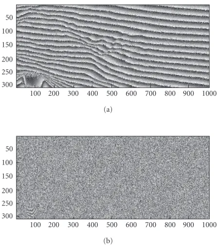
The MB-InSAR algorithm has been tested on simulated data relative to the Vesuvio area in Naples. Starting from an avail-able high-precision DEM, we simulated six acquisitions by an ERS-like system.Table 1shows the baselines. The inter-ferograms corresponding to the lowest (1–4 pair, 100 m) and highest (2–6 pair, 1050 m) baselines are shown in Figure 5 to help the reader appreciate the amount of decorrelation caused by imaging angular diversity.
The proposed algorithm, applied with respect to the pixel-to-pixel range phase differences (PD), tackles possible constant phase offset dependence in the available interfero-grams, allowing a more realistic scenario. The first baseline (−470 m) is taken as the reference, therefore the PD on the first baseline pair are the unknowns.Figure 6shows the PD evaluated from the noiseless, nonwrapped fringe pattern, as-sumed as a reference, and its histogram: note that PD asso-ciated to the flat Earth amounts to about −1.14 rads/pixel, whereas a large part of the PD is around −1.74 rads/pixel because the imaged area is located in a flank of the vol-cano.
The first experiment carried out was aimed at show-ing the reconstruction performance achievable by a sshow-ingle baseline measurement on the reference baseline PD. In par-ticular we chose the lowest baseline, that is, sensor 0–3 in Table 1. In this experiment we have also assumed no a pri-ori information about the topography, that is, we referred to the PD of a flat Earth. As a consequence we subtracted
100 200 300 400 500 600 700 800 900 1000 300
250 200 150 100 50
(a)
100 200 300 400 500 600 700 800 900 1000 300
250 200 150 100 50
(b)
Figure5: (a) Lowest and (b) highest baseline interferograms, 300
range pixels by 1000 azimuth pixels.
−10 −9 −8 −7 −6 −5 −4 −3 −2 −1 0
(b) Nr pixels
PD (rad/pixel) 101
103 105
−2 −1.8 −1.6 −1.4 −1.2 −1
PD (rad/pixel)
(a)
Figure6: (a) Wanted PD image scaled in the [−3 : 0] interval to
retain the dynamic and (b) the PD histogram.
−2 −1.8 −1.6 −1.4 −1.2 −1 PD (rad/pixel)
(a)
−11 −10 −9 −8 −7 −6 −5 −4 −3 −2 −1 0
(rad/pixel)
PD (rad/pixel) Error mean and std.
−10
−5 0
(b)
−10 −8 −6 −4 −2 0
True PD (rad/pixel)
−10
−5 0 5
Estimat
ed
P
D
(c)
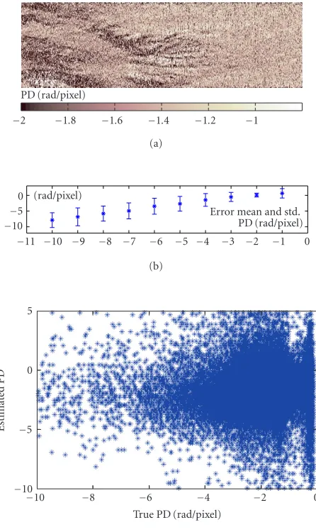
Figure7: (a) PD estimated with the lowest baseline interferograms,
(b) error plot (mean and standard deviation of the error), and (c) the scatter plot of the estimated PD versus the true PD.
the error bar plot (mean standard deviation of the error) is shown inFigure 7b. Here we see the poor quality of the re-construction due to the relatively large baseline, which is con-firmed by the appearance of a bias in the error plot for high slopes (ideally this should be horizontal) and by the presence of relatively high standard deviations, as well as high disper-sion of the scatter plot of the estimated PD versus the true PD inFigure 7c. The quality of the reconstruction improves when CB filtering was carried out: this is clearly shown in Figure 8which presents the images ofFigure 7after CB filter-ing with respect to flat Earth. Nevertheless, by lookfilter-ing at the error plot we again recognize that it is even more tilted than before, in particular, for the steepest slopes, that is, high PD, the estimates are strongly down-biased. The same con-siderations can be carried out by comparing the two scat-ter plots. Bias is eliminated when CB filscat-tering is carried out with respect to the true PD. This is clearly evident in
−2 −1.8 −1.6 −1.4 −1.2 −1
PD (rad/pixel)
(a)
−11 −10 −9 −8 −7 −6 −5 −4 −3 −2 −1 0
(rad/pixel)
PD (rad/pixel) Error mean and std.
−10
−5 0
(b)
−10 −8 −6 −4 −2 0
True PD (rad/pixel)
−10
−5 0 5
Estimat
ed
P
D
(c)
Figure8: The same asFigure 7, but with the application of the CB
with respect to the flat Earth.
Figure 9: the error bar plot is horizontal, although there is a marked dispersion. Figure 10 shows the results achieved by exploiting all the available acquisitionsandthe CB filter-ing with respect to the flat Earth. This figure, when com-pared Figure 8, shows that the introduction of large base-line interferograms has significantly deteriorated the estima-tion of high slopes (from−3 rad/pixel to−2 rad/pixel). How-ever, it also shows the effectiveness of the CB filtering; in fact, slopes close to that of the flat Earth (in bright areas) are better reconstructed when compared toFigure 8, see also Figure 6.
−2 −1.8 −1.6 −1.4 −1.2 −1 PD (rad/pixel)
(a)
−11 −10 −9 −8 −7 −6 −5 −4 −3 −2 −1 0
(rad/pixel)
PD (rad/pixel) Error mean and std.
−10
−5 0
(b)
−10 −8 −6 −4 −2 0
True PD (rad/pixel)
−10
−5 0 5
Estimat
ed
P
D
(c)
Figure9: The same asFigure 8, but with the application of the CB
with respect to the true DEM.
by the shuttle radar topography mission (SRTM) with 90 m posting and an accuracy of 15 m is a good reference for the es-timation procedure at hands.Figure 11shows the estimated PD, the mean and the standard deviation, and the scatter plot. Comparing this figure with9and10and the true one, that is,Figure 6, we appreciate the improvement in the esti-mation of both low and high slopes: the error plot bar in the middle image is thin and horizontal whereas the scatter plot is mostly concentrated around the diagonal.
7. CONCLUSIONS
A general framework that links the problem of multi-baseline SAR interferometry with the single-input multiple-output multichannel estimate has been established. We have shown that one of the most popular techniques to approach the problem, namely cross-relations, can be extended to the MB-InSAR case with slight modifications. The LS solution of
−2 −1.8 −1.6 −1.4 −1.2 −1
PD (rad/pixel)
(a)
−11 −10 −9 −8 −7 −6 −5 −4 −3 −2 −1 0
(rad/pixel)
PD (rad/pixel) Error mean and std.
−10
−5 0
(b)
−10 −8 −6 −4 −2 0
True PD (rad/pixel)
−10
−5 0 5
Estimat
ed
P
D
(c)
Figure10: The same asFigure 8, but with using all the
interfero-metric pairs.
the thus derived equation system leads to the maximization of the total energy that comes from taking all the possible in-terferograms. Not surprisingly, the outcome of this technique is that in forming each interferogram the two image pairs are prefiltered by a common band filter; such filtering cor-responds to the suboptimal spectral-shift approach already known in literature. An efficient implementation has been shown for the estimate of a constant terrain slope. The simu-lation of MB ERS-like acquisitions in rough topography has led to interesting results that reel the potential of the tech-nique.
ACKNOWLEDGMENTS
−2 −1.8 −1.6 −1.4 −1.2 −1 PD (rad/pixel)
(a)
−11 −10 −9 −8 −7 −6 −5 −4 −3 −2 −1 0
(rad/pixel)
PD (rad/pixel) Error mean and std.
−10
−5 0
(b)
−10 −8 −6 −4 −2 0
True PD (rad/pixel)
−10
−5 0 5
Estimat
ed
P
D
(c)
Figure11: (a) PD estimated with all interferograms pairs and the
application of the CB filtering with respect to the true topography. (b) The associated error plot (mean and standard deviation of the error). (c) The scatter plot of the estimated PD versus the true PD.
REFERENCES
[1] A. Ferretti, C. Prati, and F. Rocca, “Permanent scatterers in SAR interferometry,”IEEE Trans. Geosci. Remote Sensing, vol. 39, no. 1, pp. 8–20, 2001.
[2] F. Gatelli, A. Monti Guarnieri, F. Parizzi, P. Pasquali, C. Prati, and F. Rocca, “The wavenumber shift in SAR interferometry,”
IEEE Trans. Geosci. Remote Sensing, vol. 32, no. 4, pp. 855–865, 1994.
[3] G. W. Davidson and R. Bamler, “Multiresolution phase un-wrapping for SAR interferometry,”IEEE Trans. Geosci. Remote Sensing, vol. 37, no. 1, pp. 163–174, 1999.
[4] A. Monti Guarnieri and F. Rocca, “Combination of low- and high-resolution SAR images for differential interferometry,”
IEEE Trans. Geosci. Remote Sensing, vol. 37, no. 4, pp. 2035– 2049, 1999.
[5] G. Fornaro and A. Monti Guarnieri, “Minimum mean square error space-varying filtering of interferometric SAR data,”
IEEE Trans. Geosci. Remote Sensing, vol. 40, no. 1, pp. 11–21, 2002.
[6] A. Ferretti, A. Monti Guarnieri, C. Prati, and F. Rocca, “Multi baseline interferometric techniques and applications,” inProc. ESA Workshop on Applications of ERS SAR Interferom-etry (FRINGE ’96), Z¨urich, Switzerland, September–October 1996.
[7] R. Bamler and P. Hartl, “Synthetic aperture radar interferom-etry,”Inverse Problems, vol. 14, no. 4, pp. R1–R54, 1998. [8] P. A. Rosen, S. Hensley, I. R. Joughin, et al., “Synthetic
aper-ture radar interferometry,”Proc. IEEE, vol. 88, no. 3, pp. 333– 382, 2000.
[9] D. C. Ghiglia and M. D. Pritt,Two-Dimensional Phase Un-wrapping: Theory, Algorithms, and Software, John Wiley & Sons, New York, NY, USA, 1998.
[10] G. Franceschetti and G. Fornaro, “Synthetic aperture radar interferometry,” in Synthetic Aperture Radar Processing, G. Franceschetti and R. Lanari, Eds., chapter 4, pp. 167–223, CRC Press, Boca Raton, Fla, USA, 1999.
[11] H. A. Zebker and J. Villasenor, “Decorrelation in interfer-ometric radar echoes,”IEEE Trans. Geosci. Remote Sensing, vol. 30, no. 5, pp. 950–959, 1992.
[12] L. Tong and S. Perreau, “Multichannel blind identification: from subspace to maximum likelihood methods,”Proc. IEEE, vol. 86, no. 10, pp. 1951–1968, 1998.
[13] G. Xu, H. Liu, L. Tong, and T. Kailath, “A least-squares ap-proach to blind channel identification,”IEEE Trans. Signal Processing, vol. 43, no. 12, pp. 2982–2993, 1995.
G. Fornaro received the Laurea degree summa cum laude in electronic engineer-ing in 1992 and the Ph.D. degree in 1997 from the University “Federico II,” Napoli, Italy. Since 1996, he is with the “Institute for Electromagnetic Sensing of the Environ-ment” (IREA) of the Italian National Re-search Council (CNR), where he currently holds the position of Senior Researcher. In the past, he has been an Adjunct Professor
of signal theory and communication in several Italian universities: Napoli Federico II, Cassino, and Reggio Calabria. His main research interests are in the signal processing filed with applications to syn-thetic aperture radar (SAR) data processing from airborne and spaceborne systems, including motion compensation, multichan-nel SAR interferometry, differential SAR interferometry, and 3D SAR focusing. Dr. Fornaro has been a Visiting Scientist at the Ger-man Aerospace Establishment (DLR) and at the Politecnico of Mi-lano and he has been a Lecturer in several universities and interna-tional institutions such as the Istituto Tecnol ´ogico de Aeron´autica (ITA) in Sao Jos´e dos Campos (Brazil) and Remote Sensing Tech-nology Center (RESTEC), Tokyo. He is currently responsible for the Remote Sensing Unit of the Regional Center of Competence “Anal-ysis and Monitoring of the Environmental Risk” funded by the Eu-ropean Community on Provision 3.16. Dr. Fornaro was awarded (1997) the Mountbatten Premium by the Institution of Electrical Engineers (IEE).
Present and past courses included “signals and systems,” “signal theory,” “digital signal processing,” “algorithms and circuits for telecommunications,” and “radar theory and technique.” His re-search interests concern digital signal processing, mainly in the field of synthetic aperture radar signal processing. Since 1987, he has au-thored/coauthored about 100 scientific publications in the field of synthetic aperture radar. Professor Monti Guarnieri was awarded the “Symposium Paper Award” at the IGARSS’89 and the “Best Pa-per Award” at EUSAR 2004.
A. Pauciullowas born in Cercola, Italy, on October 10, 1969. He received the Dr. Eng. degree with honors in 1998 and the Ph.D. degree in information engineering in 2003, both from the University of Naples, Italy. Since 2001, he has been with the “Institute for Electromagnetic Sensing of the Environ-ment” (IREA) of the Italian National Re-search Council (CNR), where he holds a po-sition of Researcher, and since 2003, he has
been an Adjunct Professor of signal theory at the University of Cassino (Italy). His current research interests regard the field of sta-tistical signal processing with emphasis on synthetic aperture radar processing and CDMA systems.