R E S E A R C H
Open Access
Parameter estimation for SAR micromotion target
based on sparse signal representation
Sha Zhu
1,2*, Ali Mohammad-Djafari
2, Hongqiang Wang
1, Bin Deng
1, Xiang Li
1and Junjie Mao
1Abstract
In this article, we address the parameter estimation of micromotion targets in synthetic aperture radar (SAR), where scattering parameters and micromotion parameters of targets are coupled resulting in a nonlinear parameter estimation problem. The conventional methods address this nonlinear problem by matched filter, which are computationally expensive and of lower resolutions. In contrast, we address this problem by linearizing the forward model as a linear combination of elements of an over-complete dictionary. The essential idea of sparse signal representation models comes from the fact that SAR micromotion targets are sparsely distributed in the
observation scene. Accordingly, we propose to jointly estimate the target micromotion and scattering parameters via a Bayesian approach with sparsity-inducing priors. In addition, we present a variational approximation
framework for Bayesian computation. Numerical simulations demonstrate the proposed sparsity-inducing reconstruction method achieves higher resolution and better performance with smaller measures compared to conventional methods.
Keywords:synthetic aperture radar, micromotion, sparse priors, Bayesian approach, hyperpa-rameters estimation
1 Introduction
Target micromotion and micro-doppler are attracting an increasingly great interest from the synthetic aperture radar (SAR) community since they can provide addi-tional and favorable information for understanding SAR images. Micromotion is mainly embodied by rotation and vibration, and typical SAR micromotion targets include ground/ship-borne search antennas for air traffic control/surveillance [1], rotor blades of hovering heli-copters, and vibrating vehicles as well as their tires/ engines. Micromotion parameters, such as the rotating frequency and radius, record targets’attributed informa-tion. Thus their estimation is very important for micro-motion compensation and refocusing in SAR imagery, and the estimated results can also be directly used as signatures for target recognition. However, it’s a huge challenge for micromotion parameter estimation in SAR, since (1) micromotion target signals are hard to be separated from stationary-clutter ones, (2) they are also distributed over multiple range cells (especially for large
rotating radii), i.e., range cell migration (RCM) occurs, which is disadvantageous for target energy integration. Either, it’s not practical to estimate them in the SAR gray image domain because of defocusing, ghost images [2] and other energy-spread image characteristics induced by target micromotion [3].
A few algorithms have been proposed for the estima-tion of SAR micromoestima-tion targets [1,4-6]. All of them manipulate a single range cell and take micromotion target azimuthal echoes as sinusoidal frequency modu-lated (SFM) signals. The cyclic spectral density [4], a time-frequency method [6], and the adaptive optimal kernel one [5], have been used to estimate the vibrating frequency of simulated or real SAR targets. Then in [1], the wavelet or chirplet decomposition is used to sepa-rate the signal of a rotating radar dish from that of sta-tionary clutter and then auto correlation is utilized to get its rotating frequency. All these methods, however, haven’t addressed the aforementioned two key problems ever-present in SAR, i.e., clutter and RCM, which hin-ders their application in reality. In effect, unlike uni-formly moving targets, RCM correction is very difficult for micromotion ones due to their sinusoidal range his-tory [7].
* Correspondence: [email protected]
1Institute of Spatial Electronics Information, School of Electronic Science and
Engineering, National University of Defense Technology, Changsha 410073, P.R. China
Full list of author information is available at the end of the article
Matched filter is commonly used for motion or micro-motion target imaging [8,9]. It performs the reconstruc-tion at every pixel for every possible velocity of the motion, resulting in a huge space-velocity cube [8]. Worse still, for the fact that each slice of the velocity is estimated independently, it brings in ambiguous results. To improve this, an adaptive matched filtering method, called filtered back projection, was proposed by Cheney [9]. However, all these methods yield high computa-tional cost and ambiguity unavoidably caused by inde-pendent estimation. Recently, sparse signal representation and compressive sensing (CS) have become a standing interest for SAR imaging [10-13]. A joint spatial reflectivity signal inversion method based on an over-complete dictionary of target velocities was applied to SAR moving targets imaging [10]. However, large scaled matrix computation is still treated as an open problem.
Hence we propose to obtain micromotion parameters from the viewpoint of scattering center estimation, which circumvents the tough issues mentioned above via target model priors. The scattering center model, however, must herein consider target micromotion, and thus more parameters, besides target position, and higher dimensions are involved which create adverse effects on fast and global optimization. Fortunately we observe finer target s-parsity due to an increase of the parameter space dimension. Therefore we will exploit target priors and estimate the model based on sparse signal reconstruction. We recast the micro-motion tar-get imaging problem as a problem of signal representa-tion in an over-complete dicrepresenta-tionary. To enforce sparsity, we consider two Baysian prior models: generalized Gaussian andStudent-t. Then we examine the expres-sion of posterior laws, either the maximum A poseriori (MAP) estimator or the posterior means using the varia-tional Bayes approximation (VBA) [14]. Compared to conventional methods, besides overcoming two difficul-ties aforementioned, the advantages of our method include: (1) putting the micromotion target imaging and parameter estimation into a unified Bayesian parameter estimation framework, which could also handle the hyperparameter estimation; (2) breaking through the classic Relay resolution’s limit, providing the capability of super-resolution; (3) being capable of estimating micromotion parameters from limited observations; (4) being robust to noise.
The rest of the article is organized as follows. Section 2 presents the SAR signal model of micromotion targets. In Section 3 we review the different sparse modeling and optimization criteria. In particular,l1regularization
approach conducts us to the Bayesian approach which is developed in Section 4. We provide two priors as gener-alized Gaussian priors and Student-t priors, which
enforce the sparsity. Section 5 provides simulation results and performance analysis. Finally, Section 6 sum-marizes our conclusions.
2 Wavenumber-domain signal model of SAR micromotion targets
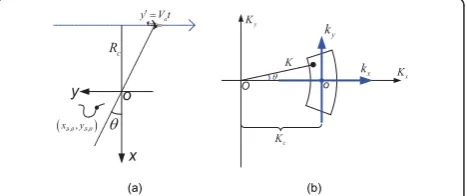
As illustrated in Figure 1, the radar moves at velocity
Va. Then for slowtimetit moves to
y=Vat=Rctanθ ≈Rcθ. (1)
We could see thatθhas the similar meaning as slow-time t. Considering an arbitrarily moving target, let vec-torϑrepresent the target micromotion parameters, such as the initial position (x, y), velocity, rotation frequency etc. Suppose the target moves to (xϑ,θ, yϑ,θ) when radar
is located at y’. f(ϑ) is the scattering coefficient. Thus the distance model of the target is
Rϑ(θ) =
(Rc+xϑ,θ)2+ (y+yϑ,θ)2
≈R2
c +y2+xϑ,θcosθ+yϑ,θsinθ.
(2)
Spotlight SAR echo of the target could be represented in the wavenumber domain as
s(K,θ;ϑ) =P(K) exp
−jK
R2
c +y2
·exp[−jK(xϑ,θcosθ+yϑ,θsinθ)],
(3)
whereP(K) is the Fourier transform (FT) of the trans-mitted signal. Then the total echoes of all targets are
Stotal(K,θ) =
f(ϑ)s(K,θ;ϑ)dϑ. (4)
After range compression and motion compensation, the first two terms of s (⋅) in Equation (3) disappear, and then the target signal model becomes
G(K,θ) =
f(ϑ) exp[−jK(xϑ,θcosθ+yϑ,θsinθ)]dϑ. (5)
x y
T
c
R a yc V t
x- T,,y- T,
o
x K y
K
K
c K
x
k
y k
T o O
(a) (b)
Figure 1Micromotion target imaging geometry. (a) The SAR
imaging geometry in slant plane and (b) the corresponding
When the target experiences micromotion, e.g., rota-tion or vibrarota-tion, we have
xϑ,θ =x+rcos(2πfmt+ϕ0), (6)
yϑ,θ =y+rsin(2πfmt+ϕ0), (7)
where micromotion parameters compose a parameter vector
ϑ(x,y,r,fm,ϕ0) (8)
and (x,y) is the position of the micromotion center,r
is the micromotion amplitude, i.e., rotating radius or vibrating amplitude, fmis the micromotion frequency, and 0 is the initial micromotion phase. Substituting Equations (6) and (7) into (5) leads to
G(K,θ)≈
f(ϑ)·h(K,θ;ϑ)dϑ, (9)
where
h(K,θ;ϑ)exp(−jK xcosθ−jK ysinθ)
·exp
−jK rcos
2πfmRc
Va
tanθ+ϕ0
.(10)
We can clearly see that, Equation (10) has an addi-tional exponential component representing target micro-motion, compared with the stationary scattering center model [5].
We now try to discretize Equation (10). Without loss of generality, suppose there areIrotated targets. Then for the ith one, let fi denotes the scatter coefficient,ϑi denotes the micromotion parameter, both of which are unknown. The model of Equation (9) could be discre-tized as
G(K,θ) =
I
i=1
fi.h(K,θ;ϑi) +εi(K,θ), (11)
where noise has been added viai(K,θ). NoteKand θ can also be discretized intoM andNvalues respectively, and therefore Equation (11) can be expressed in a matrix form as
g=Hf +ε, (12)
where
g= [G(K1,θ1),. . .,G(K1,θN),G(K2,θ1),. . .,G(K2,θN),. . .,G(KM,θ1),. . .,G(KM,θN)]T (13)
is a vector of sizeM Nrepresenting the data,
ε= [ε(K1,θ1),. . .,ε(K1,θN),ε(K2,θ1),. . .,ε(K2,θN),. . .,ε(KM,θ1),. . .,ε(KM,θN)]T (14)
is a vector of sizeM Nrepresenting the errors (model-ing and measurement),
H=
⎡ ⎢ ⎢ ⎢ ⎣
h(K1,θ1;x1,y1,r1,fm1,ϕ01)h(K1,θ1;x1,y1,r1,fm1,ϕ02. . .h(K1,θ1;xN x,yN y,rP,fQ,ϕ0J h(K1,θ2;x1,y1,r1,fm1,ϕ01 h(K1,θ2;x1,y1,r1,fm1,ϕ02. . .h(K1,θ2;xN x,yN y,rP,fQ,ϕ0J
..
. ... . .. ...
h(KM,θN;x1,y1,r1,fm1,ϕ10h(KM,θN;x1,y1,r1,fm1,ϕ20. . .h(KM,θN;xN x,yN y,rP,fQ,ϕJ0
⎤ ⎥ ⎥ ⎥ ⎦ (15)
is a matrix of dimensionsM N×NxNyPQJ represent-ing the forward modelrepresent-ing matrix system and
f={[A(xnx,xny,rp,fq,ϕ0
j)],nx= 1,. . .,Nx,ny= 1,. . .,Ny,p= 1,. . .,P,q= 1,. . .,Q,j= 1,. . .,J} (16)
is a vector of sizeNxNyPQJof parameters representing targets in the scene. In this expression A(xnx,yny,rp,fq,ϕ
0
j)is the coefficient at position(xnx,yny) with micromotion frequency fq, micromotion rangerp and initial micromotion phaseϕ0j
To this end, the problem of scattering and micromo-tion parameter estimamicromo-tion can be reformulated as a lin-ear inversion problem subject to sparsity constraints.
3 Sparse signal representation and deterministic optimization
The main idea behind sparse signal representation is, to find the most compact representation of a signal as a linear combination of a few elements (or atoms), in an over-complete dictionary [15-18]. Compared with the conventional orthogonal transform representation, this most parsimonious representation of a signal over a redundant collection of generated basis offers efficient capability of signal modeling. Finding such a sparse representation of a signal involves solving an optimiza-tion problem. Mathematically, it can be formulated as follows. For Equation (2), assumeg = H f in absence of noise whereg ÎℂM× 1is a vector of data, HÎℂM× N a matrix whose elements can be considered as an over-complete dictionary as its columns and f ÎℂN× 1 the corresponding linear coefficients. In particular,M ≪N
leads the null space of F to be non-empty such that there are many different possibilities to representgwith the elements inH. The problem of sparse representation is then to find the coefficientsf with the most few non-zero elements, i.e., ||f||0 is minimized while g =H f.
Formally,
min
f f0 s.t g=Hf (17)
where ||f||0is thel0norm which is the cardinality off. However, the combinatorial optimization problem Equa-tion (17) is NP-hard and intractable. A large body of approximation methods are proposed to address this optimization problem, such as greedy pursuit [19] based methods like matching pursuit [20], or convex-relaxa-tion [21] based methods that replace thel0 with thel1 norm,
min
Candes et al. [22] show that forK-sparsity signal that only hasKnon-zero element inf, the reconstruction of
f with M ≥ O(K log (N/K)) [15] measures can be achieved with high probability byl1 norm minimization. Moreover, to efficiently reconstruct f, the mapping matrixH should satisfy the restricted isometry property
(RIP) [23] which requires that
(1−δs)f22≤Hf 22≤(1 +δs)f 22 (19)
This RIP ofH is connected to the mutual coherence between the atoms of the dictionary which is defined as
μ(H) = max
i=j
|<ai,aj>|
aiaj (20)
where the ai is the ith column of H. Large mutual coherence indicates that there are two atoms that are closely related will degrade the reconstruction algorithm. Hence, the dictionary is required to have low coherence so that the submatrixHwithKatoms is nearly orthogo-nal [18].
If the observationgis noisy, the problem of the sparse representation for a noisy signal can be formulated as
min
f f1 s.t g−Hf
2
2≤δ, (21)
whereδis a noise allowance. Equivalently, the Equa-tion (21) can be reformulated to minimize the following objective function
L(f;λ) =g−Hf 22+λf1, (22)
wherel> 0 is the regularization parameter that bal-ances the trade-off between the reconstruction error and the sparsity off. The formulation Equation (22) can also be interpreted as the MAP estimation in the Baye-sian philosophy as we will see in the next section.
To this end, the micromotion parameter estimation is now cast as the sparse reconstruction of f associated with the parameter hypothesis at the position of non-zero elements off. There are a large number of methods to solve the Equations (21) or (22), such as the method of compressive sampling matching pursuit (CoSaMP) presented in [24] which has been widely used for its simplification and effectiveness. Here, we will compare our proposed method with this method.
4 Bayesian approach to sparse reconstruction
Even if the sparse representation has originally been introduced as an optimization problem such as Equa-tions (17), (18), (21), or (22), it can also be presented as a Bayesian MAP estimation problem [25,26]:
ˆ
f = arg max
f {p(f|g)}, (23)
where
p(f|g) = p(g|f)p(f)
p(g) ∝p(g|f)p(f), (24)
To understand this, firstly let us assume the errorin Equation (12) is centered, Gaussian and white: ε∼N(ε|0,vεI). It brings us to the expression of the likelihood:
p(g|f) =N(Hf,vεI)∝exp
− 1
2vε g−Hf
2
(25)
Secondly, choose the separable double exponential probability density [27] as the prior off:
p(f)∝exp
−α
j |
fj|
, (26)
it is then easy to see that the MAP estimation with this prior becomes
ˆ
f= arg max
f {p(f|g)}= arg minf {−lnp(f|g)}= arg minf {J(f)} (27)
with
J(f) =g−Hf 22+λf1, (28)
which can be compared to Equation (22).
The prior information that the targets are sparsely dis-tributed in the observation scene can be modeled by the two following probability density functions (PDF) [14]:
•Generalized Gaussian priors:
p(f)∝exp
⎧ ⎨
⎩−α
j
|fj|β
⎫ ⎬
⎭, (29)
which give the double exponential forb= 1 and Gaussian forb= 2 and are also more useful for sparse representation with 0 <b< 1. With these priors, the MAP estimate can be computed by optimizing the following criterion:
J(f) = 1
2vε2 g−Hf
2+α
j
|fj|β, (30)
•Student-tpriors:
p(f|ν) =
j
St(fj|ν)∝exp ⎧ ⎨
⎩−
ν+ 1 2
j
log (1 +fj2/ν) ⎫ ⎬
⎭(31)
where
St(fj|ν) =
1
√πν((ν+ 1)/2)
(ν/2) (1 +f
2
j/ν)−(ν+1)/2. (32)
These priors are interesting due to its link tol1 regu-larization and secondly due to the mixture of Gaussian representation of theStudent-t probability density:
St(fj|ν) =
∞
0
N(fj|0, 1/τj)G(τj|ν/2,ν/2)dτj (33)
which gives the possibility of proposing a hierarchical model via the positive hidden variablesτj:
⎧ ⎪ ⎪ ⎪ ⎪ ⎪ ⎪ ⎪ ⎨ ⎪ ⎪ ⎪ ⎪ ⎪ ⎪ ⎪ ⎩
p(f|τ) =
j
p(fj|τj) = j
N(fj|0, 1)τj
∝exp
−1
2
j
τjfj2
p(τj|a,b) =G(τj|a,b)∝τ
(α−1)
j exp{−βτj}
withα=β=ν/2
(34)
Using this hierarchical model, we can write the joint prior offandτ
p(f,τ) =
j
p(fj|τj)p(τj) =
j
N(fj|0, 1/τj)p(τj)
∝exp
⎧ ⎨
⎩−
1 2
j
τjfj2+ (α−1) lnτj−βτj
⎫ ⎬ ⎭
(35)
we obtain:
p(f,τ|g)∝p(g|f)p(f,τ)∝exp{−J(f,τ)} (36)
where
J(f,τ) = 1
2vε g−Hf
2
+
j
1 2τjf
2
j −(α−1) lnτj+βτj (37)
which is summarized as follows:
Joint optimization of this criterion, alternatively with respect tof (with fixedτ)
ˆ
f = arg minf{J(f,τ)}
= arg minf ⎧ ⎨ ⎩
1
2vε g−Hf
2+
j
1 2τjf
2
j
⎫ ⎬ ⎭
(38)
and with respect toτ (with fixedf)
ˆ
τ = arg minτ{J(f,τ)}
= arg minτ
⎧ ⎨ ⎩
j
1 2τjf
2
j −(α−1) lnτj+βτj
⎫ ⎬ ⎭
(39)
results in the following iterative algorithm: ⎧
⎪ ⎪ ⎨ ⎪ ⎪ ⎩
ˆ
f = [HH+vεD(τˆ)]−1Hg=D(τˆ)H(HD(τˆ)H+vεI)−1g
ˆ
τj=φ(fˆj) = a ˆ
f2
j +b
D(τˆ) = diag [1/τˆj, j= 1,. . .,n]
(40)
Note that τj is inverse of a variance and we have 1/τj=fj2+β/α. We can interpret this as an iterative
quadratic regularization inversion followed by the esti-mates of variancesτjwhich are used in the next itera-tion to define the variance matrix D(τ). This algorithm is simple to implement. However, we are not sure about its convergency. To obtain a better solution and at the same time to be able to estimate the variance of the noise, we propose to use the VBA [28-30] which con-sists in approximating the joint posterior by a separable one and then using it to do the inference.
Here we summarize this approach:
•Model for the noise:
p(g|f,vε) =N(g|Hf,vεI), τε= 1/vε
p(τε) =G(τε|αε0,βε0) (41)
•Model for the sparse signal:
⎧ ⎪ ⎪ ⎪ ⎨ ⎪ ⎪ ⎪ ⎩
p(f|v) =
j
p(fj|vj) = j
N(fj|0,vj) =N(f|0,V)
V = diag [v], τj= 1/vj, τ = diag [τ] =V−1
p(τ) =
j
G(τj|α0,β0)
(42)
•Joint posterior:
•VBA:p(f,τ,τ|g)is approximated by
q(f,τ,τε) =q(f)
j
q(τj)q(τε) (44)
where ⎧ ⎪ ⎨ ⎪ ⎩
q(f) =N(f| ˜μ,˜)
˜
μ=˜Hg=VH˜ HVH˜ +τ˜εI−1g
˜
= (τ˜εHH+V˜)−1=V˜− ˜VHHVH˜ +τ˜εI−1HV˜, with V˜= diag[˜v], (45)
⎧ ⎪ ⎪ ⎨ ⎪ ⎪ ⎩
q(τε) =G(τε| ˜αε,β˜ε)
˜
αε=αε0+ (n+ 1)/2 ˜
βε=βε0+ 1/2 ˜
τε=α˜ε/β˜ε,
(46)
⎧ ⎪ ⎪ ⎨ ⎪ ⎪ ⎩
q(τj) =G(τj| ˜αj,β˜j)
˜
αj=α00+ 1/2 ˜
βj=β00+<fj2>/2
˜
vj=β˜j/α˜j
(47)
and the expressions of the needed expectations are:
⎧ ⎪ ⎪ ⎪ ⎪ ⎨ ⎪ ⎪ ⎪ ⎪ ⎩
<f >=μ˜
<ff>=+μμ
<f2
j >= []jj+μ2j
< τ >=τ˜=α˜τ/β˜τ
<aj>=α˜j=α˜j/β˜j
(48)
This algorithm can be summarized as follows:
•Initialization:τ˜ε= 0.1, V˜ = diag[τ˜j/τ˜ε]withτ˜j= 1
•Iterations:
compute ˜ =τεH’H+V˜ −1andμ˜ =H’g
compute <fj2>=˜jj+μ˜2j
compute α˜ε,β˜εand soτ˜ε=α˜ε/β˜ε
compute α˜j,β˜jand soτ˜j=α˜j/β˜j
The only difficult and costly part is the estimation of
˜
and μ˜ . Due to the fact that we only need μ˜ and˜jj,
we propose the following approximation:
˜
μ is computed through the optimization of
J(f) =τεg−Hf2+1
2jτjfj2with respect to f and˜jj
which is the variance of fj is approximated by the empirical variance offjduring the iterations of the opti-mization algorithm.
This is the method we implemented, tested and com-pared to other classical methods.
5 Numerical experiments
In this section, we conduct several numerical experi-ments to demonstrate our method based on the sparse signal representation. The imaging geometry is shown in Figure 1. The range R0 from the original to the center of the target is 10 km, and the velocity of the platform
Vais 200 m/s. The central frequency fcis 10 GHz with bandwidth B = 400 MHz associated with the Rayleigh resolution along the range direction 0.375 m, and the angular extent of azimuth is 10° with cross-range resolu-tion 0.0861 m.
Based on the compressive sensing principle, the tar-gets can be recovered with a smaller randomly sampled measures. Figure 2 shows that sampling pattern in the wavenumber domain, the uniform sampling in Figure 2a and the randomly sampling in Figure 2b. Two targets are located at (0,0), (5,1), respectively. With the ran-domly sampled measures, Figure 3 compares the recon-struction results between the traditional method of fast FT (FFT), the CoSaMP and the Bayesian sparse method when no micromotion is present. It is shown that the CoSaMP and the proposed Bayesian method come out with clearer images and are capable to recover the true position of scatters, compared with the traditional method of FFT, even with smaller randomly measures.
When targets experience micromotion, the initial phases are assumed to be both zeros. The micromotion frequencies are 0.5, 1Hz, respectively, and the micromo-tion range is 1 and 0.5, respectively. In Figure 4b, the range profile appears clearly in the micromotion pattern compared with Figure 3b. The presentation of micromo-tion blurs the reconstrucmicromo-tion images without momicromo-tion compensation as shown in Figure 4a, while our joint parameter estimation method gains a well-focused
204 206 208 210 212 214 −20
−15 −10 −5 0 5 10 15 20
Kx
Ky
204 206 208 210 212 214 −20
−15 −10 −5 0 5 10 15 20
Kx
Ky
(a) (b)
image in Figure 4d recovering the true parameters (x,ˆ y,ˆ ˆr,fˆm,φˆ0) = (0, 0, 1, 0.5, 0), and (5,1,0.5,1,0) for the
two scatter points, respectively. Figure 4c illustrates the reconstruction result via the CoSaMP method.
We then set the micromotion range 0.5 and initial phase 0 for both targets but the micromotion frequen-cies are 0.5 and 1 Hz, respectively. We adopt the matched filtering in the 3D range-Azimuth-micromotion
frequency space by scanning a large number of possible scatterer positions and micromotion frequencies, result-ing in a large space-micromotion frequency cube. Figure 5a shows the 3D data cube. Figure 5b,c illustrate the two slices after matched filtering at micromotion fre-quencies fm= 1 Hz and fm=0.5 Hz, respectively. It is computationally expensive and not well focused being of low resolution. In addition, it is rather difficult to per-form RCM such that the position cannot be estimated accurately. In contrast, our method can overcome these drawbacks of traditional methods and yield a more pre-cise estimate.
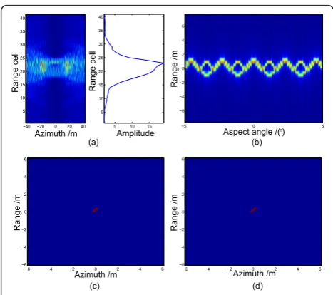
Figure 6 shows that our proposed method resolves the two very closely spaced micromo-tion targets localized at positions of (0, 0) and (0.25, 0.25), respectively. The reconstruction image by FFT is illustrated in Figure 6a and the corresponding range profile in Figure 6b. It shows that the range profiles of the two targets are overlapped so that the two targets cannot be discerned. Figure 6c,d present the imaging result of CoSaMP and our proposed Bayesian method. In contrast to the fail of conventional method as FFT, the results in Figure 6d Azimuth /m
Range /m
−6 −4 −2 0 2 4 6 −6
−4 −2 0 2 4 6
Aspect angle /(°)
Range /m
−5 0 5
−6 −4 −2 0 2 4 6
Azimuth /m
Range /m
−6 −4 −2 0 2 4 6 −6
−4 −2 0 2 4 6
Azimuth /m
Range /m
−6 −4 −2 0 2 4 6 −6
−4 −2 0 2 4 6
(a) (b)
(c) (d)
Figure 3 Reconstruction results when no micromotion is present. (a) The reconstruction image by traditional FFT in absence
of micromotion and (b) is the range profile. (c,d) The results by the
CoSaMP method and the proposed Bayesian method, respectively.
(a) (b)
Azimuth /m
Range /m
−6 −4 −2 0 2 4 6 −6
−4 −2 0 2 4 6
Target 2
Target 1
Aspect angle /(°)
Range /m
−5 0 5
−6 −4 −2 0 2 4 6
Azimuth /m
Range /m
−6 −4 −2 0 2 4 6 −6
−4 −2 0 2 4 6
Azimuth /m
Range /m
−6 −4 −2 0 2 4 6 −6
−4 −2 0 2 4 6
(c) (d)
Figure 4Reconstruction results when micromotion is present. When micromotion is present, the reconstruction image by FFT is
illustrated in (a) and the corresponding range profile is illustrated in
(b). The reconstruction results by the CoSaMP method and the
proposed Bayesian method are illustrated in (c) and (d), respectively.
Azimuth /m
Range /m
−6 −4 −2 0 2 4 6 −6
−4 −2 0 2 4 6
Target 1
Azimuth /m
Range /m
−6 −4 −2 0 2 4 6 −6
−4 −2 0 2 4 6
Target 2
Azimuth /m
Range /m
−6 −4 −2 0 2 4 6 −6
−4 −2 0 2 4 6
Azimuth /m
Range /m
−6 −4 −2 0 2 4 6 −6
−4 −2 0 2 4 6 (a)
(b) (c)
(d) (e)
Figure 5 Reconstruction results with matched filtering, CoSaMP, and the proposed Bayesian method when
micromotion is present. (a) The 3D space-micromotion frequency
data volume. (b,c) The slices atfm= 1Hz andfm= 0.5 Hz,
respectively after matched filtering. (d,e) The results by the CoSaMP
prove the super-resolution capability of the proposed method.
Figure 7 depicts the estimation root mean square (RMS) error varies with SNR which demonstrates our method can recover the targets signature parameters accurately. It can be observed that the RMS decreases sharply as the SNR increases and arrives at high
precision estimations after 0dB, indicating the robust-ness of our method to loss and noise of measurement.
6 Conclusions
In this article, we proposed a sparsity-inducing method to estimate the scattering and mi-cromotion parameters of SAR targets jointly and further formatted it in the Bayesian framework. It was done by formulating the ori-ginal nonlinear problem as a sparse representation pro-blem over an over-complete dictionary. In addition, an efficient computation algorithm as VBA estimator was applied to the hierarchical Bayesian models. The pro-posed method can exactly recover the scattering and micromotion parameters of targets, even for near spa-cing targets, achieving good performance, as demon-strated by the simulation experiments.
Acknowledgements
This work was supported by the China National Science Fund for Distinguished Young Scholars (No. 61025006) and China Scholarship Council (No. 2008611016).
Appendix CoSaMP algorithm
The basic idea of CoSaMP [24] algorithm is that: for
S-sparse signalf with S non zero elements, thez=H⋆H f can serve as a proxy for the signal whereH⋆is the Her-mitian transpose of H, since the energy in each set of S
components ofzapproximates the energy in the corre-sponding components of f. In particular, the largest S
entries of the proxyzpoint toward the largestSentries of the signalf.aThe basic steps are (appendix table):
(1)Identification:Computez¬H⋆yto find a proxy of the residual from the current samples and locate the largest componentsΩ =supp(z2S) of the proxy
z; Azimuth /m
Range cell
−40 −20 0 20 40 5
10 15 20 25 30 35 40
5 10 15 20 25 30 35 40
5 10 15
Range cell
Amplitude Aspect angle /(°)
Range /m
−5 0 5
−6 −4 −2 0 2 4 6
Azimuth /m
Range /m
−6 −4 −2 0 2 4 6 −6
−4 −2 0 2 4 6
Azimuth /m
Range /m
−6 −4 −2 0 2 4 6 −6
−4 −2 0 2 4 6
(a) (b)
(c) (d)
Figure 6 Reconstruction of two close targets when micromotion is present. For two closely localized micromotion
targets, the reconstruction image by FFT is illustrated in (a) and the
corresponding range profile in (b). The reconstruction results by the
CoSaMP method and the proposed Bayesian method are illustrated
in (c) and (d), respectively.
−015 −10 −5 0 5 10 15 20 25 30 0.5
1 1.5 2 2.5
SoCaMP Bayesian Method
−015 −10 −5 0 5 10 15 20 25 30 0.2
0.4 0.6 0.8 1 1.2 1.4 1.6 1.8 2
SoCaMP Bayesian Method
−015 −10 −5 0 5 10 15 20 25 30 0.2
0.4 0.6 0.8 1 1.2 1.4 1.6 1.8 2
SoCaMP Bayesian Method
−015 −10 −5 0 5 10 15 20 25 30 0.05
0.1 0.15 0.2 0.25 0.3 0.35 0.4
SoCaMP Bayesian Method
−015 −10 −5 0 5 10 15 20 25 30 0.05
0.1 0.15 0.2 0.25 0.3
SoCaMP Bayesian Method (a)
(b) (c)
(d) (e)
RMS
RMS
RMS RMS
RMS
SNR
SNR SNR
SNR SNR
Figure 7Reconstruction RMS. (a-e) The root mean square error versus SNR by the CoSaMP method and the proposed Bayesian method for scattering coefficient, position in range direction, position in azimuth direction, micromotion frequency and micromotion amplitude, respectively.
Appendix table The flow of CoSaMP algorithm
Input: H,g, K
Output: fˆ
f0=0
y = g k = 0
Repeat k¬k +1
z¬H⋆y Ω¬supp(z2S) T¬Ω∪supp(fk-1)
b|T←H†Tg b|Tc←0
fk¬b S y¬g-Hfk
(2)Support merger:The set of newly identified com-ponents Ωis united with the set of the components that appear in the previous approximation supp(fk-1), i.e.,T =Ω∪supp(fk-1);
(3) Estimation: Solve a least-square problem to approximate the target signal on the merged set Tof component, b|T ←H†Tg
(4) Pruning:Obtain a new approximation by retain-ing only the largest entries in this least-square signal approximation, fk¬bS;
(5)Sample update: Finally, update the residualg- H
fk .
Endnote
a
supp(z2S) represents the index set of the largest 2S ele-ments in z. H†is the Moore-Penrose pseudo-inverse of
H.
Abbreviations
SAR: synthetic aperture radar; RCM: range cell migration; SFM: sinusoidal frequency modulated; FFT: fast Fourier transform; PDF: probability density function; CS: compressive sensing; CoSaMP: compressive sampling matching pursuit; MAP: maximum A posteriori; VBA: variational Bayes approximation; RMS: root mean square.
Author details
1Institute of Spatial Electronics Information, School of Electronic Science and
Engineering, National University of Defense Technology, Changsha 410073,
P.R. China2Laboratoire des Signaux et Systèmes, UMR 8506
CNRS-SUPELEC-UNIV PARIS SUD, Supélec, 3 rue Joliot-Curie, 91192 Gif-sur-Yvette, France
Competing interests
The authors declare that they have no competing interests.
Received: 15 September 2011 Accepted: 18 January 2012 Published: 18 January 2012
References
1. T Thayaparan, K Suresh, S Qian, K Venkataramaniah, S SivaSankaraSai, KS
Sridha-ran, Micro-doppler analysis of a rotating target in synthetic aperture
radar. IET Signal Process.4, 245–255 (2010). doi:10.1049/iet-spr.2009.0094
2. BC Barber, Imaging the rotor blades of hovering helicopters with SAR, in
Proceedings of IEEE Radar Conference, Rome, Italy, pp. 652–657 (26-30 May 2008)
3. X Li, B Deng, YL Qin, YP Li, The influence of target micromotion on SAR
and GMTI. IEEE Trans Geosci Remote Sens.49, 2738–2751 (2011)
4. NS Subotic, BJ Thelen, DA Carrara, Cyclostationary signal models for the
detection and characterization of vibrating objects in SAR data, in
Proceedings of the IEEE Thirty-Second Asilomar Conference on Signals, Systems & Computers, Pacific Grove, CA, USA, pp. 1304–1308 (1-4 Nov 1998)
5. T Sparr, B Krane, Micro-doppler analysis of vibrating targets in SAR. IEE Proc
Radar Sonar Navig.150(4), 277–283 (2003). doi:10.1049/ip-rsn:20030697
6. T Sparr, Moving target motion estimation and focusing in SAR images, in
Proceedings of IEEE International Radar Conference, 2005, Crystal Gateway
Marriott, Arlington, Virginia, USA, pp. 290–294 (9-12 May 2005)
7. B Deng, GZ Wu, YL Qin, HQ Wang, X Li, SAR/MMTI: an extension to
conventional SAR/GMTI and a combination of SAR and micro-motion
techniques, inProceedings of IET International Radar Conference, Guilin,
China, pp. 1–4 (20-22 April 2009)
8. MC Wicks, B Himed, H Bascom, Tomography of moving targets (TMT) for
security and surveillance. Adv Sens Secur Appl.2, 323–339 (2006).
doi:10.1007/1-4020-4295-7_14
9. M Cheney, B Bodern, Imaging moving targets from scattered waves. Inverse
Probl.24(035005), 22 (2008)
10. I Stojanovic, WC Karl, Imaging of moving targets with multi-static SAR using
an over-complete dictionary. IEEE J Sel Top Signal Process.4, 164–176
(2010)
11. J Wang, G li, H Zhang, XQ Wang, SAR imaging of moving targets via
compressive sensing, inProccedings of IEEE International Conference on
Electrical and Control Engineering, 2010, Wuhan, China, pp. 1855–1858 (25-27 June 2010)
12. LC Potter, P Schniter, J Ziniel, Sparse reconstruction for radar. IEEE Trans Inf
Theory.52, 1030–1051 (2006)
13. S Zhu, HQ Wang, X Li, A new method for parameter estimation of
multicomponent LFM signal based on sparse signal representation, in
Proceedings of IEEE International Conference on Information and Automation,
Zhangjiajie, China, pp. 15–19 (20-23 June 2008)
14. A Mohammad-Djafari, Probabilistic models which enforce sparsity, in
Proceedings of 4th Workshop on Signal Processing with Adaptive Sparse Structured Representations 2011, ed. by C Cartis University of Edinburgh, Edinburgh, Scotland, UK, p. 107 (27-30 June 2007)
15. D Donoho, Compressed sensing. IEEE Trans Inf Theory.52, 1289–1396
(2006)
16. RG Baraniuk, V Cevher, MF Duarte, C Hegde, Model-based compressive
sensing. IEEE Trans Inf Theory.56, 1982–2001 (2010)
17. D Donoho, M Elad, V Temlyakov, Stable recovery of sparse overcomplete
representations in the presence of noise. IEEE Trans Inf Theory.52, 6–18
(2006)
18. D Donoho, X Huo, Uncertainty principles and ideal atomic decomposition.
IEEE Trans Inf Theory.47, 2845–2862 (2001). doi:10.1109/18.959265
19. JA Tropp, AC Gilbert, MJ Strauss, Algorithms for simultaneous sparse
approximation. Part I: Greedy pursuit. Signal Process.86(3), 572–588 http://
www.sciencedirect.com/science/article/pii/S0165168405002227 (2006). doi:10.1016/j.sigpro.2005.05.030
20. D Needell, R Vershynin, Signal recovery from incomplete and inaccurate
measurements via regularized orthogonal matching pursuit. IEEE J Sel Top
Signal Process.4(2), 310–316 (2010)
21. J Tropp, Just relax: convex programming methods for identifying sparse
signals in noise. IEEE Trans Inf Theory.52, 1030–1051 (2006)
22. E Candés, J Romberg, T Tao, Robust uncertainty principles: exact signal
reconstruction from highly incomplete frequency information. IEEE Trans Inf
Theory.52, 489–509 (2006)
23. J Emmanuel, E Candés, The restricted isometry property and its implications
for compressed sensing. Comptes Rendus Mathematique.346(9-10),
589–592 http://www.sciencedirect.com/science/article/pii/
S1631073X08000964 (2008). doi:10.1016/j.crma.2008.03.014
24. D Needell, JA Tropp, CoSaMP: iterative signal recovery from incomplete and
inaccurate samples. Appl Comput Harmon Anal.26(3), 301–321 (2008)
25. A Mohammad-Djafari, Bayesian inference for inverse problems in signal and
image processing and applications. Int J Imaging Syst Technol Spec Issue
Comput Vis.16(5), 209–214 (2006)
26. J Tropp, Sparse Bayesian learning and the relevance vector machine. J
Mach Learn Res.1, 211–244 (2001)
27. PM Williams, Bayesian regularization and pruning using a Laplace prior.
Neural Comput.7, 117–143 (1995). doi:10.1162/neco.1995.7.1.117
28. VŠmidl, A QuinnP,The Variational Bayes Method in Signal Processing,
(Springer, Berlin, 2005)
29. CM Bishop,Pattern Recognition and Machine Learning, (Springer, New York,
2006)
30. C Chaux, PL Combettes, JC Pesquet, RW Valérie, A variational formulation
for frame-based inverse problems. Inverse Probl.23(4), 1–28 (2007)
doi:10.1186/1687-6180-2012-13