Volume 2006, Article ID 35352, Pages1–16 DOI 10.1155/ASP/2006/35352
Spectrally Efficient Communication over Time-Varying
Frequency-Selective Mobile Channels: Variable-Size
Burst Construction and Adaptive Modulation
Francis Minhthang Bui and Dimitrios Hatzinakos
The Edward S. Rogers Sr. Department of Electrical and Computer Engineering, University of Toronto, 10 King’s College Road, Toronto, ON, Canada M5S 3G4
Received 1 June 2005; Revised 10 March 2006; Accepted 15 March 2006
Methods for providing good spectral efficiency, without disadvantaging the delivered quality of service (QoS), in time-varying fading channels are presented. The key idea is to allocate system resources according to the encountered channel. Two approaches are examined: variable-size burst construction, and adaptive modulation. The first approach adapts the burst size according to the channel rate of change. In doing so, the available training symbols are efficiently utilized. The second adaptation approach tracks the operating channel quality, so that the most efficient modulation mode can be invoked while guaranteeing a target QoS. It is shown that these two methods can be effectively combined in a common framework for improving system efficiency, while guaranteeing good QoS. The proposed framework is especially applicable to multistate channels, in which at least one state can be considered sufficiently slowly varying. For such environments, the obtained simulation results demonstrate improved system performance and spectral efficiency.
Copyright © 2006 Hindawi Publishing Corporation. All rights reserved.
1. INTRODUCTION
Achieving high spectral efficiency is an important goal in communication. However, it is equally important that the quality of service (QoS), quantified by the bit error rate (BER), will not deteriorate as a result of this goal. We propose strategies that allocate resources for improving the spectral efficiency, while maintaining good QoS, for burst-by-burst communication systems. In these systems, data are transmit-ted in bursts or blocks, possibly with training and other types of symbols to aid data recovery at the receiver. Over any such burst, the channel is assumed to be sufficiently constant or stationary, that is, a single channel environment is approxi-mately experienced by the entire data burst (also known as a quasi-static or block-fading channel). The rationale for em-ploying burst transmission is that since the channel is ap-proximately the same over the entire received burst, it can be estimated, and a single time-invariant equalizer can be used to mitigate interferences for all data symbols within a single burst. In other words, the various data bursts can be indepen-dently processed at the receiver, on a burst-by-burst basis.
Unfortunately, with the advent of the systems employ-ing high-frequency carriers and used in high-speed envi-ronments, the quasi-static channel assumption is becoming more questionable. Essentially, the channel can be regarded
as constant over a burst if the burst duration is less than the channel coherence timeTC. However, the channel coherence
time is itself actually a statistical measure, whose precise for-mula depends on the definition criterion. Loosely speaking, [1,2],
TC≈
1
fm (1)
or alternatively, defined as the time over which the time cor-relation function is above 0.5 [1,2],
TC≈
9 16π fm
, (2)
where fmis the maximum Doppler shift given by
fm=vm
λ = vmfc
c (3)
withvmbeing the mobile speed,λthe wavelength,fcthe
car-rier frequency, andcthe speed of light. The relationship with the burst duration can also be viewed using the normalized Doppler shift fmTS, whereTSis the symbol duration. Then,
using (1), a burst is within a coherence time if the number of symbols in the burst, that is, the burst sizeBS, is
BS<
1 fmTS.
20 10 0 −10 −20 −30 −40
Re
ce
iv
ed
en
ve
lo
p
e
(d
B
)
0 1 2 3 4 5 6 7 8
×104
Data symbol (a) 20
0 −20
−40
−60
Re
ce
iv
ed
en
ve
lo
p
e
(d
B
)
0 1 2 3 4 5 6 7 8
×104
Data symbol (b)
Figure1: Received envelopes over fading channels at carrier frequency fc = 3.5 GHz: (a) mobile speedvm =100 km/h, or normalized maximum Doppler shiftfmTS=5.55×10⁻⁴; (b)vm=10 km/h, or fmTS=5.55×10⁻⁵.
Regardless of which definition, (1) or (2), is used, the co-herence time TC is inversely proportional to the both
car-rier frequency fc and the mobile speedvm. Hence, with an
increase of the carrier frequency fc in modern systems, TC
tends to become shorter. In practice, the burst duration is chosen to be significantly less than TC in order to justify
the quasi-static assumption. For example, in GSM [1,2], a burst duration is 0.577 ms, whileTC≈11 ms (using (1) with
fc=960 MHz,v=100 km/h).
With an increased carrier frequency, for example,fc<3.5
GHz in the developing IEEE802.20 standard, the coherence time reduces toTC≈3.6 ms, and with target bitrates on the
order of 1 Mbps, the symbol durationTS ≈ 2μs(assuming
2 bits/symbol, e.g., using 4-QAM [2,3]). Hence, the normal-ized Doppler shift is fmTS ≈ 5.55×10⁻⁴, and a coherence
time contains at a maximum 1/(fmTS)=1800 symbols.
For visualization purposes,Figure 1shows typical fading envelopes versus the symbol index for the above calculated normalized Doppler shift fmTs ≈5.55×10⁻⁴, and also for
fmTs≈5.55×10⁻⁵. Here, the time variations are described
by the Jakes power spectral density (see (7)). The smaller nor-malized Doppler shift corresponds to a more slowly varying channel.
In coping with the reduced coherence timeTC, a
num-ber of approaches can be considered. First, the channel in-variance assumption can be eliminated, and new receiver structures can be designed. However, suppose that such changes are not permissible, for example, due to existing infrastructure or hardware constraints. Then, the question is whether basic burst-by-burst techniques can still be used in rapidly time-varying channels. We examine techniques for achieving reliable communications in such channels, while
still using the same basic burst-by-burst receiver methodol-ogy.
Ultimately the goal is to shorten the burst duration in some manner, so that it remains within the coherence dura-tion. Following are example methods that can be considered. (S1) Reduce the number of data symbols per burst
To reduce the overall burst duration, the symbol duration TSmust not be increased. With this solution, the
transmis-sion efficiency, that is, the ratio of useful data symbols over all symbols in a burst, can be severely affected, especially in rapidly varying channels.
(S2) Reduce the burst duration
Alternatively, the same number of symbols in a burst can be maintained, but the symbol duration TS is reduced. While
the transmission efficiency is maintained, if the symbol du-ration is too short relatively to the channel delay spread, the channel becomes highly frequency selective, with severe in-tersymbol interference (ISI). The use of a high-complexity equalizer would be needed for acceptable QoS.
(S3) Use a variable-size burst approach
over which the channel is slowly changing will be exploited to use a larger burst. As will be seen inSection 3, this enables a better use of the available training symbols for improved transmission efficiency and QoS. Moreover this construction can be achieved entirely at the receiver.
If the channel quality is further known for each burst, it is also possible to adapt the modulation mode for the data symbols on a burst-by-burst basis. When the channel is be-nign or of good quality, a higher-order modulation constel-lation, for example, 16-QAM, can be used for efficiency while still maintaining a good QoS, defined by a target BER. How-ever, when the channel is hostile or of poor quality, a lower-order modulation mode, for example, BPSK, is selected to maintain an acceptable QoS. Known as adaptive modula-tion [3,5], this methodology permits an overall improve-ment in spectral efficiency. Thus, adaptive modulation plays a key role in balancing the system’s integrity and efficiency in a time-varying environment.
As will become evident in the remainder of the paper, the overall conclusion of this work is the following: if the underlying time-varying channel can be modeled as multi-state, where at least one state is slowly varying, then reliable communication is still possible using conventional burst-by-burst techniques when coupled with a variable-size burst-by-burst ap-proach. Furthermore, the spectral efficiency can be enhanced with the use of adaptive modulation. When combined to-gether, these two strategies deliver an attractive framework, with minimal modifications of existing systems, for reliable and efficient communication over time-varying channels.
When there is no slow state in the underlying channel, the transmission efficiency is poor since the burst size needs to be very small. By combining variable-size burst construc-tion with basis-expansion modeling (BEM) of the channel [6,7], the transmission efficiency can be improved. However, in this case, the system complexity is increased due to more complicated estimation and equalization procedures. With some performance loss, the complexity can be reduced sig-nificantly using time-varying FIR equalization [8]. But more importantly, even with the addition of basis-expansion mod-eling, the variable-size burst methodology remains applica-ble [6]. This is because, under certain conditions, BEM es-sentially allows a rapidly varying channel to be treated as an equivalent slow fading channel. In fact, at the cost of system complexity, the BEM modification only improves the flexi-bility of variable-size burst construction, making it applica-ble to a wider range of time-varying channels [6]. In the in-terest of brevity and clarity, this work will thus focus on burst construction, and the integration with adaptive modulation, all using conventional channel modeling.
The rest of this paper is organized as follows. After de-scribing a mobile channel model with multistate consider-ations in Section 2, a variable-size burst structure is pre-sented inSection 3. Channel equalization technique and es-timation techniques are then outlined in Section 4. These techniques are subsequently incorporated into a channel-tracking framework for constructing variable-size bursts in Section 5. And to further improve the spectral efficiency, an adaptive modulation method coupled with variable-size
burst construction is discussed inSection 6. Next, to demon-strate the performance of the proposed methods, simulation results are obtained inSection 7. Lastly, conclusions are made inSection 8.
2. CHANNEL MODEL
2.1. Mobile fading channels
In this paper, time-varying frequency-selective mobile fading channels are assumed. Under the well-known wide-sense sta-tionary uncorrelated scatterers, (WSSUS) assumptions [2,9], such channels can be viewed as equivalent time-varying FIR filters, with impulse response
h(t,τ)=
P−1
p=0 αp(t)δ
τ−τp
, (5)
wherePis the number of observable paths, as will asτpand
αp(t), respectively, the delay and gain of thepth path.
The time variations, due to the Doppler effect as men-tioned inSection 1, are described for each of thePpaths by the autocorrelation function [9]:
rp(τ)=σp2J0
2π fmτ
(6) or, equivalently, in the frequency domain, by the Jakes power spectral density:
Sp(f)=
⎧ ⎪ ⎪ ⎪ ⎨ ⎪ ⎪ ⎪ ⎩
σ2 p
π fm 1−
f / fm
2, |f|< fm, 0, |f|> fm,
(7)
whereσ2
pis the average power of thepth path,J0(·) the zero-order Bessel function of the first kind, and fmthe maximum
Doppler shift. Note that the coherence timeTC from (2) is
defined based on (6).
The channel frequency selectivity is described by specify-ing the average power for each of the path coefficientsαp(t),
resulting in the power-delay profile. For example, a typical urban (TU) COST207-type [3,9] channel power-delay pro-file with four observable paths is shown inFigure 2, with pa-rameters summarized inTable 1.
2.2. Multistate extension
While the above mobile channel model is both time and fre-quency selective, it essentially describes one single channel stateor environment, where a state is characterized by a par-ticular fm. FromSection 1, fm is dependent on the mobile
velocityvmfor a fixed carrier frequency fc. Hence, as a user
changes his or her mobile activities, the perceived operating environment is also effectively modified. In the context of a variable-size burst, it is beneficial to model such activities explicitly, since the goal is to exploit low-mobility activities for efficiency. To this end, we consider a multistate channel model, where each state is defined by an associated Doppler shift fmor mobile speedvm. Evidently, the more states
0.8 0.7 0.6 0.5 0.4 0.3 0.2 0.1 0
N
o
rm
aliz
ed
path
po
w
er
0 0.5 1 1.5 2 2.5 3 3.5 4 Path delay (μs)
Figure2: Normalized power-delay profile for a 4-path typical ur-ban (TU) COST207-type channel, with parameters summarized in
Table 1.
Table1: Normalized power-delay profile for a typical urban (TU) COST207-type channel, as depicted inFigure 2.
Delay position (μs) Path power
0 0.7236
1.54 0.1554
2.31 0.0720
2.69 0.0490
Suppose the user’s mobile activities are such that there areκdistinguishable states:{k1,k2,. . .,kκ}. Denote the
prob-ability of the user being in thekistate asp(ki), so that κ
i=1
p(ki)=1. (8)
To fully describe the user’s mobile behavior as a function of time, the joint probability mass function (pmf) needs to be specified as a function of the current state, and the past state(s), that is, memory consideration. However, for sim-plicity, we assume in this paper a memoryless model. Then, the channel states for various time instants can be considered discrete i.i.d random variables, with the pmf specified by
p(ki), i=1,. . .,κ. (9)
Note that when considering a quasi-static channel approxi-mation, the probability of the channel for any burst being in a certain state is specified by (9), that is, on a burst-by-burst basis.
2.3. A Two-state channel example
As an example of a channel with two states, when using a Gauss-Markov approximation to the Jakes model, consider the following composite Gauss-Markov channel, used previ-ously in [4]. Denote the channel taps for thenth time instant
20 10 0 −10 −20 −30 −40
Re
ce
iv
ed
en
ve
lo
p
e
(d
B
)
0 400 800 1200 1600 2000 2400
Data symbol (a) 10
0 −10 −20 −30 −40
Re
ce
iv
ed
en
ve
lo
p
e
(d
B
)
0 400 800 1200 1600 2000 2400
Data symbol (b)
Figure3: Quasi-static channel approximation forfmTS=1×10⁻³ using: (a) fixed-size bursts of 100 symbols; (b) fixed-size bursts of 400 symbols.
ashn. Let the two states bes-state andf-state. Then the
chan-nel changes between time instants as
hn=νηshn−1+us
+1−νηfhn−1+uf
, (10)
whereνis a Bernoulli random variable,ηs,ηf the correlation
coefficients for each state, andus,uf the noise terms. Hence,
by appropriately assigning values toηsandηf, the channel
can be considered as composing of a slow and a fast state, with state probabilities specified by the Bernoulli rvν.
For the above composite Gauss-Markov model, each state is specified by parameters relating to the associated Doppler shift fm, for example,s-state byηs. In this paper, each channel
state is described more generally using (6) and (7). 3. VARIABLE-SIZE BURST STRUCTURE
A variable-size burst structure, based on a conventional fixed-size burst, is described in this section.
3.1. Motivation
As mentioned inSection 1, the idea of using a burst trans-mission system originates from approximating the channel as constant or quasi-static over some interval, which should be less than the coherence time. In the context of a time-varying mobile channel, Figure 3illustrates this approximation on a channel with normalized Doppler shift fmTS = 1×10⁻³
Training Data Guard interval
G1 G2 = G3 G4 = G5 = G6 G7 = G8
H1 H2 H3 H4
(a) Transmitted
burst
Received burst
(b)
Received burst
Received burst
Received burst
Received burst (c)
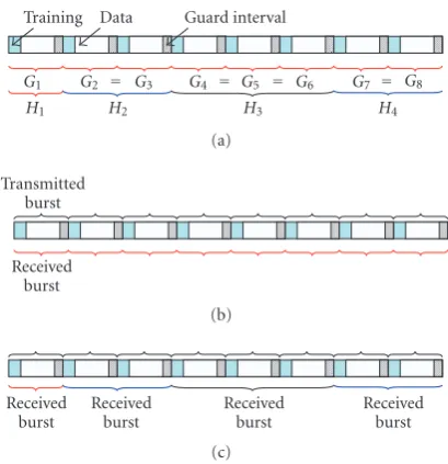
Figure4: Variable-size burst structure with preamble training sym-bols: (a) quasi-static channel approximations for each burst, where some channels may be the same, for example,G2 = G3 ≡ H2;
(b) fixed-size burst system, assuming all channels are different; (c) variable-size (received) burst system, exploiting knowledge of chan-nel similarities.
the channel using a total of 24 fixed data bursts. The larger burst approximates the same channel using fewer data bursts, a total of 6 in this case. With a fixed overhead of train-ing symbols per burst, it is more desirable to use the larger burst, since the transmission efficiency (which is propor-tional to the spectral efficiency) would be higher. However, as illustrated byFigure 3(b), the larger-burst approximation is quite inaccurate at certain times, for example, the deep fade around symbol 1000 is missed entirely. On the other hand, the smaller burst is rather redundant at certain times, for ex-ample, over the symbol range 1200–1500, a single-burst ap-proximation suffices. Hence, a compromise between the two different burst sizes, using a variable-size burst, is advanta-geous in terms of efficiency.
3.2. Accumulated received burst structure
Figure 4shows a potential variable-size burst structure. The key idea here is to realize the distinction between a transmit-ted and a received burst: regardless of what the transmitter sends, the receiver ultimately can make a choice on what it considers a received burst (used for further processing, such as channel estimation). Then, the transmitter simply trans-mits fixed-sizefundamentalbursts. At the receiver, a variable-size burst is constructed by combining consecutive trans-mitted fundamental bursts appropriately. For this scheme to function, as in a fixed-size burst system, the fundamental bursts need to satisfy the quasi-static channel conditions. The difference is that, by tracking the channel, the receiver can de-tect a slowly changing duration, and accordingly adapts the burst size by combining the consecutive fundamental bursts
within this duration. The result is a largeraccumulatedburst, composed of fundamental bursts, with an enlarged set of training symbols delivering a more accurate channel estima-tion.
3.3. Example construction
To illustrate the described procedure,Figure 4(a) shows an example scenario, where the channels for eight consecutive fundamental bursts are designated: G1,G2,. . .,G8. A fixed-size burst receiver simply assumes that these channels are all different and constructs received bursts of the same size as the transmitted bursts as shown inFigure 4(b). However, if the underlying channels are not all different, then a variable-size burst can combine appropriate consecutive fundamental bursts to form larger accumulated bursts, while still satisfying the quasi-static assumption. For example, ifG2 =G3,G4 = G5=G6,G7=G8 (seeFigure 3, e.g., of how this may arise), then the unique channels can be re-designated asH1,H2,H3, H4, from which there would be four enlarged variable-size accumulated bursts as inFigure 4(c).
3.4. Comparisons to a fixed-size burst
From a transmitter perspective, there is essentially no diff er-ence in terms of the burst structure. The fundamental burst size is still specified by the highest-speed fm. However, in
rapidly time-varying channels, the variable-size burst struc-ture is more attractive, because it has the potential to main-tain good spectral efficiency.
Indeed, consider using solution (S1), fromSection 1, to reduce the number of data symbols per burst. Then, to main-tain the same transmission efficiency, the number of train-ing symbols must also be reduced. However, estimation and equalization depend on the raw number of training sym-bols (and not the transmission efficiency). Hence, a fixed-size burst, which in general has insufficient training symbols in rapidly time-varying channels, will suffer from significant performance degradation due to unsuccessful channel esti-mation and equalization. By contrast, a variable-size burst has the potential to regain the performance loss by making the best use of the available training symbols.
The effect of training-symbol assignment or placement is not investigated here. While optimal training placement can have a significant impact on the overall performance [10], the present paper has a different perspective: given a train-ing regime (e.g., preamble, midamble, or superimposed), the problem is how to combine the available training symbols from different bursts in an advantageous manner, notably by tracking the channel. This is based on the assumption that more training symbols would yield better overall per-formance.
4. CHANNEL EQUALIZATION AND ESTIMATION
First, we will describe the ideal minimum mean-square (MMSE) equalizer, assuming knowledge of the channel. Then, using training symbols, a maximum-likelihood (ML) estimator provides an estimate of the channel. Through-out this section, it is assumed that the accumulated burst is already received under quasi-static channel conditions. InSection 5, the channel estimation and equalization tech-niques described here will be incorporated in a framework for constructing a quasi-static accumulated burst.
4.1. MMSE equalization
Consider the typical equivalent baseband signal representa-tion
y[n]=
L−1
l=0
h[n;l]x[n−l] +v[n], (11)
where x[n] is the transmitted symbol at instant n, y[n] the received symbol,h[n;l] the channel impulse response,L the channel length (assumed known), andv[n] the additive white Gaussian noise (AWGN) with varianceσ2
v. When the
channel is time invariant as in a burst-by-burst system, the dependence ofh[n;l] onnis suppressed:
y[n]=
L−1
l=0
h[l]x[n−l] +v[n]=h[n]x[n] +v[n], (12)
wheredenotes convolution. In this case, a matrix formula-tion can be obtained. At the instantn, for the potential recov-ery of thenth symbolx[n],Nconsecutive received symbols are collected as
y(n)=Hx(n) +v(n) (13) withy[n]=[y[n],. . .,y[n−N+1]]T,v[n]=[v[n],. . .,v[n−
N+ 1]]T,x[n]=[x[n],. . .,x[n−N−L+ 2]]T,
H= ⎡ ⎢ ⎢ ⎢ ⎢ ⎣
h[0] · · · h[L−1] · · · 0 . ..
0 · · · h[0] · · · h[L−1] ⎤ ⎥ ⎥ ⎥ ⎥
⎦, (14)
where (·)Tdenotes matrix transpose, andHhas dimensions
N×(N+L−1).
Using the minimum mean-squared error (MMSE) cri-terion, a linear equalizerf =[f[0],f[1],. . .,f[N−1]]T is
found by minimizing the cost function JMSE(f)=EfHy(n)−x[n−δ]
2
, (15)
whereE(·) denotes the expectation operator, (·)H the
Her-mitian transpose, andδ is a delay, with permissible values δ =0,. . .,N+L−1 (see (18) and (19) for the effect ofδ). The solution to (15) is [11]
f=R−1p, (16)
whereR=E(y(n)yH(n)),p=E(x∗[n−δ]y(n)) are known,
respectively, as the autocorrelation and cross-correlation. Making the independence assumption of data symbols at dif-ferent instants, then
R=σx2HHH+σv2IN, p=σx2H1δ+1, (17) where σ2
x = E(|x[n]|2) is the symbol energy,σv2 the noise
variance,IN theN×N identity matrix, and1δ an all-zero vector except for theδelement, which is equal to 1 (hence, in (17),1δ+1extracts the (δ+ 1)th column ofH).
Given a fixed channel matrixH[11], MMSE(δ−1)=σ2
x
1−1H
δHHΔ−1H1δ
, (18)
where Δ = HHH +σ2
v/σx2IN. Hence, the optimalδ can be
found by evaluating Ξ=diagσ2
x
IN−HHΔ−1H (19) from which (δ−1) corresponds to the row number ofΞwith the minimum value (e.g., if the first row element is the min-imum, the delay isδ=0).
4.2. ML channel estimation
The channelh[n] can be estimated using an ML estimator, with training symbols. This is ultimately where the variable-size burst advantage is realized: a larger accumulated burst provides more training and thus better channel estimate.
Consider the first fundamental burst in an accumulated burst, withM consecutive training symbols located by the index setI1= {k,. . .,k+M−1}, that is,x[k],. . .,x[k+M−1] are known symbols. The received signal is
yI1=xI1h+vI1, (20) whereyI1=[y[k+L−1],. . .,y[k+M−1]]T,vI1 =[v[k+
L−1],. . .,v[k+M−1]]T,h=[h[0],. . .,h[L−1]]T,
xI1=
⎡ ⎢ ⎢ ⎢ ⎢ ⎣
x[k+L−1] · · · x[k] ..
. ...
x[k+M−1] · · · x[k+M−L+ 1] ⎤ ⎥ ⎥ ⎥ ⎥
⎦. (21)
Note that when preamble training and zero-padding guard intervals are used (seeFigure 4), then the dimensions of the above quantities can be enlarged for better estimation. If x[k−L+1],. . .,x[k−1] correspond to the guard symbols and are thus known to be all equal to zero, then the received signal can be formed asyI1 =[y[k],. . .,y[k+M−1]]T, with
burst,
⎡ ⎢ ⎢ ⎢ ⎢ ⎣
yI1
. ..
yIμ ⎤ ⎥ ⎥ ⎥ ⎥ ⎦=
⎡ ⎢ ⎢ ⎢ ⎢ ⎣
xI1
. ..
xIμ ⎤ ⎥ ⎥ ⎥ ⎥ ⎦h+
⎡ ⎢ ⎢ ⎢ ⎢ ⎣
vI1
. ..
vIμ ⎤ ⎥ ⎥ ⎥ ⎥
⎦ (22)
or
yΣ=xΣh+vΣ. (23) The ML channel estimate is
hML=x†ΣyΣ, (24)
where (·)†denotes the Moore-Penrose pseudoinverse [11].
5. CHANNEL TRACKING FOR VARIABLE-SIZE BURST
In this section, the described quasi-static estimation and equalization methods will be incorporated into a threshold-based scheme for detecting channel changes. A receiver pro-cedure for processing variable-size bursts is also presented. 5.1. Threshold-based change detection
The variable-size burst construction problem can be stated iteratively. Suppose that, at the current iteration, the accu-mulated burstBcurrent is composed ofμconsecutive funda-mental bursts,Bcurrent= {bk,. . .,bk+μ−1}, and that the chan-nel is the same over the entireBcurrent. Then, upon the recep-tion of the candidate fundamental burstbk+μ, the choices are
the following.
(H1) Addbk+μ to the current accumulated burst, forming Bpotential = {bk,. . .,bk+μ}. Continue withbk+μ+1 as the next candidate.
(H2) Rejectbk+μ, terminateBcurrent, and accept it as the best choice. Reinitialize withbk+μas the start of a new
ac-cumulated burst.
To decide whether to accept (H1) or (H2), the following pro-cedure is performed.
(1) In (24), estimate the channel usingBcurrent, returning an estimatehC.
(2) Similarly, estimate the channel usingBpotential, return-ing an estimatehP.
(3) Compute the squared norm of the estimation diff er-ence:
ρed=hC−hP 2
. (25)
(4) Compare to a thresholdρthfor detection decision:
ρed−ρth H2 H1
0. (26)
In the above,ρed is a second-order measure of the channel change in the following sense. Suppose that the underlying channel of Bcurrent is h, and that hC is a close estimate of the true channel. Then ifbk+μ experiences the sameh, the
resulting estimation difference
hed=hC−hP (27) is small (in some norm). But if the channel has changed for the candidatebk+μ, the estimation differencehedis large. In (25), a squared norm is used to quantify this difference. The utility of this choice is made evident by examining (29) and (30), as explained next.
5.2. Threshold function selection
Let the true channel beh, then depending on the detection decision (i) or (ii), the channel estimation errorhceis either hce,C = h−hCorhce,P = h−hP. The channel estimation
error is unknown, since the truehis not available. However, an upperbound for its squared norm can be approximated as follows. Noting that|hed|2= |hce,C−hce,P|2and assuming
independence of the estimation errors, so thatE(h∗ce,Chce,P)=
E(hce,Ch∗ce,P)=0,
Ehed 2
≈Ehce,C 2
+Ehce,P 2
≥Ehce 2
(28) which means that by keeping the estimation differencehed small as in (26), the resulting channel estimation errorhce should also be statistically small.
Next, consider the effect of a channel estimation error, with impulse responsehce[n], at the equalizer input. From (12),
y[n]=h[n]x[n] +v[n]
=h[n]−hce[n]
x[n] +
v[n]
hce[n]x[n] +v[n] =h[n]x[n] +v[n] +v[n],
(29)
whereh[n] is the estimated channel impulse response (i.e., corresponds to eitherhC orhP depending on the detection decision). Hence for an equalizer using the estimated chan-nelh[n], the second term v[n], due to the channel estima-tion error, can be viewed as an addiestima-tional noise source. For a particular channel realization, this estimation noise error has variance:
Ehce[n]x[n]2
=σx2 L−1
l=0
hce[l]2
=σx2ρce, (30)
where σ2
x is the average symbol energy. From (29), when
noise is significant (low SNR), a small estimation error does not necessarily deliver significant performance gain. How-ever, at high SNR, the channel estimation error becomes the bottleneck. In fact, it is well known that channel estimation error can result in an error floor at high SNR [11]. Hence, with a fixed average symbol energyσ2
x, the channel
estima-tion error variance (30) should be proporestima-tional to the chan-nel noise varianceσ2
v for optimal performance tradeoff.
ρth: threshold for decision.
Ntotal: total number of fundamental bursts to be processed.
bsizemax: max. number of fundamental bursts in the
accumulated burst.
s: fundamental burst defining start of the current accumulated burst.
(I)Initialization (1) Sets=1 (II)Iteration
fori=2, 3,. . .,Ntotal
if (i−s+ 1≥bsizemax) or (i=Ntotal),
(1) Set current accumulated burst= all fundamental bursts fromstoi, (2) Equalize the current accumulated burst, (3) Resets=i+ 1,
else if (ρed> ρth),
(1) Set current accumulated burst=
all fundamental bursts fromstoi−1, (2) Equalize the current accumulated burst (3) Resets=i,
end end
Algorithm1: Variable-size burst receiver with channel tracking.
improvement compared to a fixed-size burst in time-varying environments, the effect of threshold optimization will not be explored. Instead, inSection 7, a sensibly predetermined threshold function ρth, weighted against the noise variance σ2
v, will be used to assess potential improvement.
5.3. Receiver processing with a variable-size burst
Implicit in the tracking procedure is the requirement of a buffer for computing the intermediateh1andh2, which in-troduces additional complexity and also latency. To allevi-ate the incurred penalties, a maximum burst size can be im-posed. Fortunately, as evidenced inSection 7, a modest burst size can yield significant performance gain. In fact, when the receiver already has sufficient training to equalize the chan-nel accurately, that is, approaching the MMSE lower-bound, enlarging the accumulated burst does not produce further appreciable improvement. Also, constraining the burst size minimizes the propagation of estimation errors. At low SNR, with inaccurate channel estimates, tracking can erroneously accumulate more fundamental bursts than possible, thus vi-olating the quasi-static requirement.
Accounting for the above factors,Algorithm 1shows a conceptual receiver procedure for processing variable-size bursts. Essentially, while the accumulated burst has not ex-ceeded the maximum size, the receiver iteratively considers consecutive candidate fundamental bursts for inclusion, us-ing a threshold-based change detection scheme.
5.4. Constrained optimization interpretation
Let the objectiveF(μ)=Mμbe the total number of training symbols as a function ofM, the number of training symbols
in a fundamental burst (see (20)), andμ, the number of fun-damental bursts in the accumulated burst (see (22)). Note thatMis typically a fixed constant, defined by the training density. Also, lethibe the channel associated with theith fun-damental burst in the accumulated burst. Then variable-size burst construction is equivalent to a mixed-integer optimiza-tion problem: [12].
Lemma 1. There exists a unique solution to the following burst construction problem:
maximizeF(μ)=Mμ
subject toμ∈Z(an integer); μ≤bsizemax, h1=h2= · · · =hμ(channel invariance).
(31)
Proof. The result follows trivially by noting that F(μ) is a strict monotonic increasing function of μ. Hence, con-strained to a bounded domain, there exists a unique maxi-mum.
Remarks
If, instead, the objective function is the training density, where the number of training symbols can be adapted per burst, then the optimization problem is not necessarily mixed integer (andM represents essentially a step-size pa-rameter). However, in this case the transceiver design would be more complicated, with some form of feedback required.
Since the existence of a unique solution is guaranteed by Lemma 1, an iterative search for the solution can be imple-mented. Here, the main difficulty is ensuring that the chan-nel invariance constraint in (31) is maintained. The chanchan-nels
hiare not known, and estimateshi must be used. Then in the presence of noise and estimation error, with probabil-ity one,h1 =h2 = · · · = hμ, for allμ. Hence, consider in-stead the equivalent form of the constraint|hi+1−hi|2=0, i=1,. . .,μ−1 yielding the squared norm relaxation [12]
hi+1−hi2
< ρth, i=1,. . .,μ−1, (32) where ρth is a small constant, allowing for some flexibility in accommodating channel estimation error. Essentially, this entails choosingρthas inSection 5.2.
Also, at thekth iteration, instead of simply checking|hk−
hk−1|2against the threshold,|hC−hP|2as defined by (25) is used to guarantee the constraint. This allows for improved estimation consistency since more training symbols are used for estimation with more iterations.
Algorithm 1implements the described strategy to itera-tively search forμ, which approaches the optimal solution in the squared norm sense.
6. ADAPTIVE MODULATION
(1) At the receiver, perform a channel-quality measure-ment, returning a channel metric.
(2) Relate this channel metric to a suitable modulation mode, which yields the highest throughput while maintaining the required level of QoS.
(3) Signal the selected modulation mode to the transmit-ter to be used in the next transmission burst.
Note that the average transmitted symbol energyσ2 x can
be kept the same, regardless of the modulation mode in use. This alleviates the need of power control, which is typical for alternative systems operating in fading channels. The QoS is nonetheless guaranteed, by using the suitable modulation mode for an operating channel quality. In addition, the sym-bol rate is maintained constant so that the required band-width is unchanged, regardless of the selected modulation mode.
6.1. Channel metric
The most accurate metric for quantifying the channel qual-ity is the BER. However, since the BER is often difficult to estimate directly, alternatives are often used instead. For a frequency-non selective or flat-fading channel, the short-term signal-to-noise ratio (SNR) is an appropriate metric [3, 13]. For a frequency-selective channel, the short-term SNR is inadequate, since the influence of ISI must be taken into account. Moreover the BER performance for frequency-selective channel is a complicated function of many factors, including channel length, power-delay profile, and even the form of equalizer used, for example, the number-taps in a linear equalizer, and the value of the equalizer delay. In the following, we outline three possible approaches for comput-ing a channel metric, which can be used to guarantee a target QoS by selecting the appropriate modulation mode. (1) Exact residual ISI
Given enough side information, the exact probability of er-ror can be computed. Consider the overall equalized channel impulse response:
g[n]=f∗[n]h[n], (33) where f[n] andh[n] are the impulse responses of the equal-izer and the channel, respectively. Following [14], consider the equalizer output at instantn
z[n]= f∗[n]y[n] =g[δ]x[n−δ] +
k =δ
g[k]x[n−k] +
N−1
k=0
f∗[k]v[n−k], (34) where the first term is the desired signal component, the second term the residual ISI, and the last term the equal-ized noise. Note thatg[n] is effectively an FIR filter of length N+L−1. Hence, for a particular input sequencexJofN+L−1
symbols, the corresponding residual ISI term is DJ=
k =δ
g[k]xJ[n−k]. (35)
When usingM-PAM, the resulting probability of error is [14]
PM
DJ
=2(M−1)
M Q
⎛ ⎜ ⎝
g[δ]−DJ2 σ2
n
⎞ ⎟
⎠, (36)
whereσ2
nis the variance of the equalized noise
σ2 n=σv2
N−1
n=0
f[n]2
. (37)
Hence, for a particular channel, input sequence andM, the exact probability of error can be found. A channel metric can then be defined as
ΓISI=DJ, (38)
and the appropriate modulation mode, that is, the value of M, can be determined from (35) for a desired QoS. Unfortu-nately, this exact metric is not practical, since knowledge of N+L−1 data symbols surrounding the desired symbolx[δ] is required (which implies knowledge of the entire sequence of data).
Alternatively, an average and an upper-bound probability of error can be found, respectively, as [14]
PM=
xJ PM
DJ
PxJ, (39)
PM
DJ∗
, D∗J =(M−1)
k =δ
g[k], (40)
where (39) is an average over all possiblexJ, and (40) is due to the worst-case residual ISI. Unfortunately, the former is computationally expensive, while the latter tends to be rather loose. In addition, for a fading environment, averaging over all fading-channel realizations is required. Thus the exact residual ISI metric is only appropriate for channels with very short length.
(2) Pseudo-SNR
The pseudo-SNR is basically the SNR at the equalizer output: pseudo-SNR= wanted signal power
residual ISI + noise power, (41) and is defined in terms of the coefficients of a decision-feedback equalizer in [3]. Using a linear MMSE equalizer with delayδ,
ΓpSNR= σ 2 xg[δ]
2
σ2 x
$
k=δg[k] 2
+σ2 n
(42)
for a particular channel realization, whereσ2
(37). Note that as in [3], a Gaussian approximation of the residual ISI term is made, and independence of the residual ISI and noise is assumed. Then the BER formula in an AWGN channel can be used. For example, the BER for a particular channel realization with 4-QAM:
PΓpSNR
=P4-QAM(awgn)
ΓpSNR
=Q ΓpSNR
, (43)
and more importantly the BER over a mobile fading channel can be found, for a specificm-QAM mode, as
P(mf)m-QAM( ¯γ)= %∞
0 P (awgn) m-QAM
ΓpSNR
pΓpSNR, ¯γ
dΓpSNR, (44) where ¯γis the average channel SNR:
¯
γ=Eh[n]x[n] 2
Ev[n]2 , (45)
Pm(awgn)-QAM(·) the AWGN BER expressions for the m-QAM mode (e.g., can be found in [3,14]); andp(ΓpSNR, ¯γ) the pdf of the pseudo-SNRΓpSNRover all fading channel realizations, at a certain average channel SNR ¯γ. In general, the closed-form pdf is not available, and the (discretized) pdf needs to be computed numerically, at each ¯γof interest [3]. With ΓpSNRas a channel metric, the appropriatem-QAM mode is selected from (44) for a target QoS.
(3) MSE-based metric
The pseudo-SNR metric requires knowledge of the channel h[n]. For methods that find the equalizerfdirectly without estimatingh[n], a channel metric can be defined based on the MSE computed at the equalizer output [5]. In the sequel, the relationship between the MSE-based metric and the pseudo-SNR is established.
At the equalizer output (34),
z[n]= f∗[n]y[n]=x[n−δ] +e[n], (46)
wherex[n−δ] is the desired component, ande[n] the over-all residual equalization error, which, combines residual ISI, equalized noise, and also scaling. Then, the MSE is the equal-ization error variance,
σ2
e =Ee[n] 2
=Ex[n−δ]−z[n]2, (47)
and can be estimated using training symbols [5]. A corre-sponding channel metric is
ΓMSE= σ 2 x
σ2 e
. (48)
Table2: Threshold-based switching rules for adaptive modulation.
Switching criterion Modulation mode
0≤ΓC< t1 V1
t1≤ΓC< t2 V2
..
. ...
tQ−1≤ΓC<∞ VQ
Making the assumption of independence between data symbols, residual ISI, and noise,
ΓpSNR= σ2
xg[δ] 2
σ2
e −σx2g[δ]−1
2. (49) Comparing (48) and (49), the two metrics are identical when g[δ]=1, which occurs when the ISI is completely suppressed by the equalizer (at high SNR).
In general, the relationship between the probability of er-ror and MSE is not expressible in a simple closed form. But an upperbound can be obtained [15],
Pe
σ2
e
≤exp
&
−1−σe2/σx2
σ2 e
'
. (50)
Then, the same approach as (44) applies, using the pdf of ΓMSE, which is close to the pdfΓpSNRat high SNR.
6.2. Threshold-based mode adaptation
Consider a general channel metric ΓC, for example,ΓC =
ΓpSNR, which quantifies in some manner the operating chan-nel quality. A threshold-based scheme can be constructed as follows [3, 5]. Designate the choice of available mod-ulation modes by Vq, q = 1,. . .,Q, where Q is the total
number of available modulation modes;V1is the constella-tion with the least number of points (most robust); andVQ
the highest (most efficient). ThenTable 2shows the switch-ing rules, based on a set of thresholds (t1,. . .,tQ−1), where t1< t2 <· · · < tQ−1are chosen to guarantee some required level of QoS [3].
6.3. Thresholds selection
For a set of thresholds (t1,. . .,tQ−1), the mean throughput (number of bits per symbol) [3,16]
B( ¯γ)=BV1
%t1
0 p
ΓC, ¯γ
dΓC
+
Q−1
q=2 BVq
%tq
tq−1
pΓC, ¯γ
dΓC
+BVQ %∞
tQ−1
pΓC, ¯γ
dΓC,
(51)
Ntotal: total number of fundamental bursts to be processed.
s: starting fundamental burst of current accumulated burst.
γC: a channel quality metric (e.g.,ΓpSNR).
(I)Initialization (1) Sets=1,
(2) Measure channel metricγCusingsth fundamental burst,
(3) Request QAM-mode(γC) to transmitter for the rest of current accumulated bursts.
(II)Iteration
fori=2, 3,. . .,Ntotal
Track channel starting fromsth fundamental burst (using tracking strategy fromSection 5,
Algorithm 1) ..
.
if (channel change detected atith fundamental burst) (1) Set current accumulated burst=
all fundamental bursts fromstoi−1, (2) Decode the current accumulated burst,
(3) Resets=i(i.e., start of new accumulated, burst) (4) Measure channel metricγCusingsth
fundamental burst,
(5) Request QAM-mode(γC) to Tx for the rest of the new accumulated burst. end
end
Algorithm2: Adaptive modulation with variable-size burst.
(e.g., throughput of 16-QAM is 4 bps). In a fading channel, the average BER for adaptive modulation
PAM(mf )( ¯γ)= 1 B( ¯γ)
( BV1
%t1
0 P (awgn) V1
ΓC
pΓC, ¯γ
dΓC
+
Q−1
q=2 BVq
%tq
tq−1
P(awgn)Vq
ΓC
pΓC, ¯γ
dΓC
+BVQ %∞
tQ−1
P(awgn)VQ
ΓC
pΓC, ¯γ
dΓC
) .
(52)
Hence, with (52), the thresholds can be optimized to produce a desired QoS, for example, using a cost function based on desired BER and average throughput [3,16].
6.4. Integration with variable-size burst construction
A two-layer strategy is used for adaptation: variable-size burst construction in the first layer, and adaptive modula-tion method in the second. Feedback is required only in the second layer. A conceptual algorithm for this strategy is sum-marized inAlgorithm 2.
Note that the channel quality is measured once per accu-mulated burst, that is, the metric obtained with the starting fundamental burst selects the modulation mode for the en-tire accumulated burst. This is valid because, with channel tracking, the same channel condition, that is, same channel quality, applies to the entire burst.
6.5. Proof of optimality
Let the objective G(q) = log2q be the throughput (num-ber of transmitted bits per symbol) as a function of the modulation modeq. For simplicity, let us assume that there are four modulation modes, that is, q = 0 (no transmis-sion), 2 (BPSK), 4 (4-QAM), 16 (16-QAM). Then adaptive modulation with variable-size burst is equivalent to
maximizeG(q)=log2q,
subject toμ∈Z(an integer), μ≤bsizemax, h1=h2= · · · =hμ(channel invariance),
BER(μ,q),≤BERmax, q∈ {0, 2, 4, 16}, σ2
x=constant,
(53)
where BERmax specifies the maximum acceptable bit-error rate for a desired QoS, andσ2
x = E(|x[n]|2) is the symbol
energy.
Proposition 1. Under the constraints in(53), the given joint optimization problem of burst construction and adaptive mod-ulation has a unique solution. Moreover, the joint optimization is actually separable, that is, burst construction and adaptive modulation can be performed separately in a two-layer strat-egy.
Proof. (i) The objectiveG(q) is a strict monotonic increasing function ofq.
(ii) When channel estimation is performed using train-ing symbols, BER is also a function of μ. Under the first three constraints, essentially those from (31), the accumu-lated burst constructed has more training symbols and also satisfies quasi-static channel requirements. Then, BER is a strict monotonicdecreasingfunction ofμ.
(iii) Under the last constraint of constant symbol energy, BER is a strict monotonicincreasingfunction ofqsince in-creasingqdecreases the minimum distance between constel-lation points.
(iv) From (i), (ii), and (iii), a unique solution exists on a bounded domain.
(v) Moreover, to optimally satisfy the fourth BER con-straint, μneeds to be as large as possible (for anyq). This means that optimization of burst size (which depends on the underlying channel, not on the modulation-mode) can be performed first, followed by the modulation mode search (recall that burst construction deals with channel rate of change, while adaptive modulation addresses the channel quality).
optimalqcan then be searched from the given mode choices, producing the largestqthat satisfies the BER constraint. Remarks
The channel invariance constraint is crucial. Otherwise, if the channel changes between bursts, then increasing the num-ber of training symbols or the modulation mode may or may not improve estimation, depending on the operating channel SNR. In other words, without this constraint, the monotonicity of BER(μ,q) may no longer hold. As such, nonunique local maxima may exist on the BER surface over the bounded domain, and the problem would no longer be separable.
Proposition 2. For each modulation mode q, there is a bi-jection (one-to-one and onto mapping) between the (pseudo-SNR) channel metric and the BER.
Proof. This should be quite obvious by construction of any channel metric, because otherwise the constructed metric is not a good metric at all. For the specific case ofΓpSNR, the pseudo-SNR metric, the key is to realize that bothΓpSNRand BER are continuous and strict monotonic decreasing func-tions of the average channel SNR ¯γ, evident from (42), (44), and (45).
In other words, there existφ,ψ : BER =φ( ¯γ),ΓpSNR = ψ( ¯γ), whereφ,ψ are both bijective (forφ, see (44)). Being bijections,φ,ψ have bijective inverses: ¯γ = φ−1(BER), ¯γ = ψ−1(Γ
pSNR). Then,ΓpSNR=ψ(φ−1(BER)).
Theoretically,Proposition 2implies that, when using the channel metricΓpSNRto maintain the BER constraint in (53), the equivalent condition isΓpSNR(μ,q)≤tq(BERmax), where tq(·)=ψ(φ−1(·)), for eachq. However, note that the above is
a purely existential construction, since it is usually difficult to compute the inverses in closed form, for example, comput-ing ¯γfrom BER using (44). Therefore, in practice, the opti-mal thresholds are usually determined empirically for adap-tive modulation [3,16], as discussed inSection 6.3.
With the above considerations,Algorithm 2implements a two-layer strategy that iteratively searches for the opti-mal (μ,q). The switching thresholds (with guaranteed op-timal existence by Proposition 2) are empirically approxi-mated and used according toTable 2 for adaptive modula-tion.
Remarks
Due to the particular forms of the objective and constraints considered here, the optimization can be decoupled as two separate layers. However, this is not always possible. Chang-ing the objective function, for example, addition of delay cost, may necessitate cross-layer optimization. In addition, with more extensive solution spaces (larger bsizemax and more mode choices), an exhaustive search quickly becomes prohibitively complex due to the combinatorial nature of the
mixed-integer problem. For all these cases, suboptimal tech-niques, such as convexification and relaxation [12], may be applied to reduce complexity.
6.6. Metric errors
It is important to realize that optimality of the above tech-niques is only guaranteed under ideal situations. In practice, estimation errors lead to constraint violations and therefore suboptimal solutions. In particular, with respect to adaptive modulation, not only can metric errors occur due to insuffi -cient training, delays in transceiver feedback also mean that transmitter mode switching may be too slow.
Algorithm 2 implements closed-loop metric signalling [3], and thus has a minimum latency of one fundamental burst. In other words, even without feedback delay, the met-ric estimated using the current burst is not used to update the modulation mode until the next transmitted burst, during which time, depending on the Doppler frequency, the chan-nel quality may have changed significantly. In real applica-tions, with feedback delay, the actual latency is even higher. Especially when the channel is changing rapidly, this latency can cause incorrect modes to be invoked by the transmitter receiving outdated metrics.
Under certain conditions, it may be possible to predict the upcoming metrics, thus mitigating the latency effect. Var-ious important considerations in practical implementations of adaptive modulation are surveyed in [3]. InSection 7.5, the effect of latency in the metric estimation will be evalu-ated by simulation.
7. SIMULATION EXAMPLES
Simulation parameters used are: carrier frequency fc =
3 GHz, symbol durationTS = 2μs, fundamental burst size
= 80 symbols, training density =10% (i.e., 8 symbols per fundamental burst), normalized data symbols withσ2
x = 1,
4-QAM for fixed-modulation simulations, number of equal-izer taps N = 50. The power-delay profile is exponential (same shape asTable 1), with delay positions [0, 4, 6, 7]×TS,
so that the channel lengthL=8.
The maximum accumulated burst size bsizemaxequals 4 fundamental bursts. The threshold function ρth is defined piece-wise over the SNR-rangeη∈[0, 40] dB:
ρth(η)= ⎧ ⎪ ⎪ ⎪ ⎪ ⎪ ⎨ ⎪ ⎪ ⎪ ⎪ ⎪ ⎩
4σ2
v, η≤20,
2σ2
v, 20< η≤30,
σ2
v, 30< η≤40,
(54)
whereσ2
v is the channel noise variance. This threshold
100
10−1
10−2
10−3
10−4
10−5
10−6
BER
0 5 10 15 20 25 30 35 40
Average channel SNR MMSE
Variable-size burst Fixed small burst
Fixed big burst Quasi-static burst
Figure5: BER performance over fading channel with fmTs =1× 10⁻⁴or mobile speedv
m=18 km/h.
7.1. Variable-size burst in a slow-fading channel
Here, the channel is characterized by one Doppler state, with fmTs = 1×10⁻⁴ or mobile speed vm = 18 km/h.Figure
5 shows the resulting BER performances for the following schemes.
(1) MMSE
Obtained using a fixed-size burst equal to the fundamental burst, and witha prioriknowledge of the channel. This is the lower-bound for other cases.
(2) Quasi-static burst
Also obtained using a fixed-size fundamental burst, but with an estimated channel. There is insufficient training for accu-rate estimation, manifested by a large performance gap from the lower bound.
(3) Fixed small burst
Obtained using a fixed-size burst equal to two fundamental bursts. More training symbols are available compared to the quasi-static burst, resulting in performance improvement. (4) Fixed big burst
Obtained using a fixed-size burst equal to four fundamental bursts. This scheme approaches the MMSE performance at low SNR, but suffers from an error floor at high SNR due to quasi-static violation being a bottleneck in the absence of noise.
100
10−1
10−2
10−3
10−4
10−5
10−6
BER
0 5 10 15 20 25 30 35 40
Average channel SNR MMSE
Variable-size burst Fixed small burst
Fixed big burst Quasi-static burst
Figure6: BER performance over fading channel with fmTs =9× 10⁻⁴or mobile speedv
m=162 km/h.
(5) Variable-size burst
Inherits the best characteristics of the previous two fixed-size burst schemes, with good performance at low SNR and no error floor at high SNR.
7.2. Variable-size burst in a fast-fading channel
Here, fmTs = 9×10⁻⁴, corresponding tovm = 162 km/h.
Figure 6shows the resulting performances. Due to construc-tion, the MMSE and quasi-static burst have identical perfor-mances as before. In this more rapidly varying scenario, both fixed-size burst schemes suffer from error floors. By contrast, the variable-size burst is able to compensate for the faster channel changes, without being affected by an error floor due to quasi-static violations. Although not as significant as in a slow fading scenario, the variable-size burst still delivers bet-ter performance compared to a quasi-static burst.
7.3. Variable-size burst in a two-state fading channel
As described in Section 2.2, the channel here has two Doppler states: a slow statek1 with fmTs = 1×10⁻⁴, and
a fast state k2 with fmTs = 9×10⁻⁴. In other words, this
channel is a combination of the previous two scenarios. The state probabilities are p(k1) = 0.8 and p(k2) = 0.2. This channel is characteristic of a user who spends most of the time in a low-mobility environment, for example, around the vm=18 km/h range.Figure 7shows the results.
100
10−1
10−2
10−3
10−4
10−5
10−6
BER
0 5 10 15 20 25 30 35 40
Average channel SNR MMSE
Variable-size burst Fixed small burst
Fixed big burst Quasi-static burst
Figure7: BER performance over fading channel with 2 Doppler states:k1with fmTs =1×10⁻⁴andk2with fmTs =9×10⁻⁴; the state probabilities arep(k1)=0.8 andp(k2)=0.2.
performance gain by exploiting the slower channel state, without being affected by an error floor due to the fast state. 7.4. Average burst length of the variable-size burst
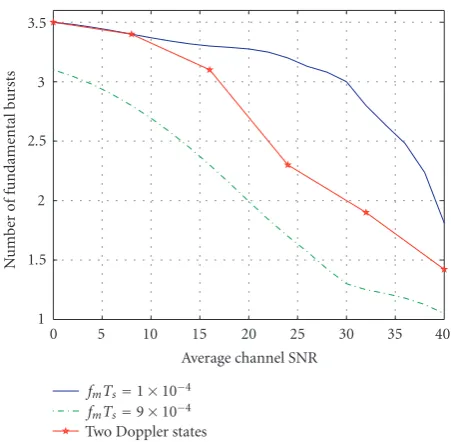
Figure 8shows the average burst length in the previous chan-nel settings. In a slow fading chanchan-nel, the burst is closer to the maximum admissible length (bsizemax=4). But in a fast fading channel, the burst length tends to be shorter in order to satisfy the quasi-static assumption. In a two-state channel, the average burst length is somewhere in between, regulated essentially by the threshold functionρth.
7.5. Adaptive modulation: BER performance
The previous simulations show that the two fixed-size burst schemes severely fail in a two-state channel, even with fixed modulation. Hence, we will focus on the MMSE, quasi-static and variable-size bursts for adaptive modulation.
The pseudo-SNR metricΓpSNR is used with thresholds and associated modulation modes summarized inTable 3.
Transmission blocking (no transmission) is invoked for very poor conditions. The highest-throughput mode is 16-QAM, transmitting 4 bits/symbol. To illustrate the effect of metric errors as discussed inSection 6.6, two cases are con-sidered: (i) no feedback delay, resulting in (minimum) la-tency of 1 burst; (ii) feedback delay of 2 bursts, causing over-all latency of 3 bursts.Figure 9shows the resulting BER per-formances.
Without feedback delay, the MMSE scheme is able to limit the maximum BER to 10−4, for the SNR range greater than 15 dB. By modifying the thresholds, this range can be changed accordingly, but at the loss of throughput efficiency
3.5
3
2.5
2
1.5
1
N
u
mber
of
fundamental
bursts
0 5 10 15 20 25 30 35 40
Average channel SNR
fmTs=1×10⁻⁴
fmTs=9×10⁻⁴ Two Doppler states
Figure8: Average burst length (in terms of number of fundamental bursts) of a variable-size burst.
Table3: Switching thresholds for adaptive modulation.
Channel metric (dB) Modulation mode 0≤ΓpSNR<8 No transmission
8≤ΓpSNR<12 BPSK
12≤ΓpSNR<20 4-QAM
20≤ΓpSNR<∞ 16-QAM
(Figure 10). The obtained results reveal variable-size burst as superior to the fixed-size scheme, guaranteeing a better QoS quantified by the BER.
With delay, the overall QoS is lowered for all cases. This reduction is more noticeable at low SNR since an erroneous metric here implies incorrect invocation of a higher-order mode. By contrast, at high SNR where a higher-order mod-ulation mode is usually already appropriate, an incorrect invocation causes less degradation. And as mentioned in Section 6.6, in certain cases, it may be possible to perform metric prediction to mitigate latency [3].
7.6. Adaptive modulation: throughput performance
A complete comparison of various burst schemes, when us-ing adaptive modulation, also requires examinus-ing the corre-sponding throughputs (number of bits per symbol), depicted inFigure 10.
10−1
10−2
10−3
10−4
10−5
BER
0 5 10 15 20 25 30 35 40
Average channel SNR MMSE
MMSE (delayed) Variable size
Variable size (delayed) Quasi-static Quasi-static (delayed) Figure9: Adaptive modulation BER performance over fading chan-nel with 2 Doppler states:k1 with fmTs = 1×10⁻⁴ andk2 with
fmTs = 9×10⁻⁴; the state probabilities are p(k1) = 0.8 and
p(k2)=0.2.
4 3.5 3 2.5 2 1.5 1 0.5 0
Thr
o
ug
hput
(bps)
0 5 10 15 20 25 30 35 40
Average channel SNR MMSE
MMSE (delayed) Variable size
Variable size (delayed) Quasi-static Quasi-static (delayed) Figure10: Adaptive modulation throughput performance corre-sponding toFigure 9.
transmission blocking are observed for the variable-size and quasi-static bursts. The reason is that, at low SNR, an accu-rate channel metric is not available for optimal modulation mode selection. At high SNR, all schemes have nearly iden-tical throughputs, since the estimation of channel metric is more accurate without noise.
The combined BER and throughput performances dem-onstrate the superiority of a variable-size burst compared
to its fixed-size counterpart. It maintains almost identical throughput, but supports much improved QoS.
8. CONCLUDING REMARKS
In this work, two approaches for efficient and reliable com-munications in time-varying mobile environments are pre-sented: variable-size burst construction and adaptive mod-ulation. It has been shown that, when the underlying time-varying channel is dominated by a slower state, reliable and efficient communication is still possible using a conventional burst-by-burst receiver methodology.
If the channel is dominated by a fast channel state, the variable-size burst performance approaches that of the quasi-static burst, with poor QoS and efficiency. For these sce-narios, as mentioned in Section 1, the variable-size burst methodology can be combined with basis-expansion chan-nel models to deliver improved performance at the cost of complexity [6].
ACKNOWLEDGMENTS
The authors thank the anonymous referees whose insight-ful reviews were instrumental in improving the paper. We are also grateful to the Editor Professor Geert Leus for sug-gesting important modifications. This work was supported by the Natural Sciences and Engineering Research Council of Canada. Some of the material in this paper was presented at IEEE Globecom 2004, Dallas, Tex.
REFERENCES
[1] T. S. Rappaport,Wireless Communications: Principles and Prac-tice, Prentice Hall, Englewood Cliffs, NJ, USA, 1996.
[2] R. Steele and L. Hanzo,Mobile Radio Communications: Second and Third Generation Cellular and WATM Systems, John Wiley & Sons, New York, NY, USA, 1999.
[3] L. Hanzo, C. Wong, and M. Yee,Adaptive Wireless Transceivers: Turbo- Coded, Turbo-Equalized and Space-Time Coded TDMA, CDMA, and OFDM Systems, John Wiley & Sons, New York, NY, USA, 2002.
[4] F. M. Bui and D. Hatzinakos, “A receiver-based variable-size-burst equalization strategy for spectrally efficient wire-less communications,”IEEE Transactions on Signal Processing, vol. 53, no. 11, pp. 4304–4314, 2005.
[5] F. M. Bui and D. Hatzinakos, “Adaptive modulation using variable-size burst for spectrally efficient interference sup-pression in wireless communications,” inProceedings of IEEE Global Telecommunications Conference (GLOBECOM ’04), vol. 2, pp. 898–902, Dallas, Tex, USA, November-December 2004.
[6] F. M. Bui and D. Hatzinakos, “Identification and tracking of rapidly time-varying mobile channels for improved equaliza-tion: a basis-expansion model approach,” to appear inThe 5th International Symposium on Communication Systems, Network and Digital Signal Processing (CSNDSP ’06), Patras, Greece. [7] G. B. Giannakis and C. Tepedelenlioglu, “Basis expansion