Volume 2011, Article ID 425203,9pages doi:10.1155/2011/425203
Research Article
ISAR Imaging of Ship Target with Complex Motion Based on New
Approach of Parameters Estimation for Polynomial Phase Signal
Yong Wang and Yi-Cheng Jiang
Research Institute of Electronic Engineering Technology, Harbin Institute of Technology, Harbin 150001, China
Correspondence should be addressed to Yong Wang,[email protected]
Received 25 September 2010; Revised 20 January 2011; Accepted 9 March 2011
Academic Editor: M. Greco
Copyright © 2011 Y. Wang and Y.-C. Jiang. This is an open access article distributed under the Creative Commons Attribution License, which permits unrestricted use, distribution, and reproduction in any medium, provided the original work is properly cited.
ISAR imaging of ships at sea with significant motion results in the Doppler frequency shift for the received signal is time-varying, which will deteriorate the ISAR image quality for the Range-Doppler (RD) algorithm. In this paper, the received signal is modeled as a multicomponent cubic phase signal (CPS), and a new method for estimating the parameters of CPS based on the integrated high-order matched phase transform (IHMPT) is proposed. This algorithm is simpler and more computational efficient than some of other parameters estimation algorithms proposed previously. Then, combined with the Range-Instantaneous-Doppler (RID) technique, the high quality instantaneous ISAR images can be obtained. The results of simulated and measured data are provided to demonstrate the effectiveness of the new method proposed.
1. Introduction
The Inverse Synthetic Aperture Radar (ISAR) technique has attracted the attention of many scholars all around the world, and many useful results have been obtained in the past
two decades [1–4], especially for the ISAR imaging of plane
target. The ISAR imaging of ship target is also very important in the national defense, such as the target recognition and
battlefield awareness [5, 6]. The imaging condition for
ship target is more complicated than the plane due to the extreme sea environment. This sea-induced motion results in chaotic, complex, three-dimensional (3D) motion and does not conform to the ISAR imaging assumptions of planar, constant rate rotation. In this case, the Doppler frequency shift for the received signal is time-varying, which will deteriorate the ISAR image quality for the Range-Doppler (RD) algorithm.
The Range-Instantaneous-Doppler (RID) algorithm was
presented for ISAR imaging of maneuvering target in [7–
10], where the Doppler analysis for RD algorithm is replaced
by the time frequency analysis, such as the DechirpClean
method [11], the Radon-Wigner transform [12], and the
adaptive Chirplet decomposition algorithm [13]. These
algorithms are based on the assumption that the received
signal in a range bin is a multicomponent linear-frequency-modulated (LFM) signal, and the instantaneous ISAR images can be obtained by estimating the parameters of it. Hence, these algorithms are suitable in situations where the maneu-verability is not too severe. For the ship target with high
maneuverability, the algorithms presented in [11–13] will
not be appropriate for the sake of high-order phase term
in the received signal. In [14, 15], the received signal is
modeled as multicomponent cubic phase signal for the ship target, and a TC-DechirpClean algorithm was presented to estimate the parameters of it. But this algorithm requires a two-dimensional maximization to estimate the parameters
of the cubic phase signal, and it therefore suffers from a
high computational load. In [16], the product high-order
matched-phase transform (PHMT) is proposed for ISAR imaging of ship target by the authors. By the multiplication of high-order matched-phase transform slices for the cubic
phase signal at different time positions, the parameters of
the multicomponent cubic phase signal can be estimated. But the selection and total number of time positions will
influence the parameters estimation accuracy. In [17,18], the
x
y z
R(x1,y1,z1)
P β Ω
Figure1: Geometry of ISAR image for ship target.
In this paper, the received signal is modeled as mul-ticomponent cubic phase signal (CPS), and the integrated high-order matched phase transform (IHMPT) is presented to estimate the parameters of it. This method requires only one-dimensional maximization, and the parameters
of each component can be estimated efficiently. Then, the
high-quality instantaneous ISAR images can be obtained combined with the RID technique.
This paper is organized as follows. InSection 2, the cubic
phase signal model for the received signal of ship target in
ISAR imaging is established; in Section 3, the principle of
IHMPT is presented, and the ISAR imaging algorithm of
ship target based on the IHMPT is discussed in Section 4;
the results for simulated and measured data are given in Section 5;Section 6is the conclusion for the paper.
2. Cubic Phase Signal Model for the
Received Signal
In this section, we assume that the motion compensation (including the range alignment and phase adjustment) has been completed, and the ISAR imaging geometry for ship
target is shown inFigure 1.
In Figure 1, the coordinate of the radar line-of-sight
(LOS) isxyzand the synthetic vectorΩdenotes the angular
velocity of the target. Thexaxis is located on thez−Ωplane,
and the unit vector of LOS isr, which overlaps thezaxis. The
pointOis the rotating centre of the ship target, and we use
the vectorR(x1,y1,z1) to denote the position of a scatterer
Pon the target. The Doppler frequency shift of the scatterer
induced by the rotation can be written as [8]
ω=4π
λ [(Ω×R)•r], (1)
whereλis the wavelength of the radar,×denotes the outer
product, and•denotes the inner product.
For ship target with high maneuverability, the synthetic
vectorΩcan be approximated as follows:
Ω≈Ω0+α0t+γ0t2, (2)
whereΩ0,α0, andγ0are the constant term, first-order term,
and second-order term coefficients ofΩ, respectively.tis the
azimuth time. Then, we can rewrite (1) as follows:
ω=4π
λ [(Ω×R)•r]=
4π
λ [Ω•(R×r)]
=4π
λ
Ω0•μ+α0•μt+γ0•μt2
,
(3)
whereμ = R×r. Then, for the Doppler frequencyω, the
received signal for scattererPcan be written as
s0(t)=A0exp
jωt
=A0exp
j4π
λ
Ω0•μt+α0•μt2+γ0•μt3 , (4)
whereA0is the amplitude. From (4), we can see that for a
scatterer on the ship target, the received signal has the form of cubic phase signal (CPS). Hence, for multiple scatterers in a certain range bin, the received signal can be characterized as
s(t)= K
k=1
Akexp
j4π
λ
Ω0k•μkt+α0k•μkt2+γ0k•μkt3
= K
k=1
Akexp
jak,1t+ak,2t2+ak,3t3
,
(5)
where
ak,1=
4π
λ
Ω0k•μk,
ak,2=
4π
λ
α0k•μk,
ak,3=
4π
λ
γ0k•μk,
(6)
andK is the number of scatterers in a range bin,Ak (k =
1, 2,. . . K) is the amplitude of each scatterer, andak,l|3l=1are
the phase coefficients to be determined.
It can be seen from (5) that the received signal in a
0 2000 4000 6000 8000
0 100 200 300 400 500 Relative third-phase derivative
R
elati
ve
amplitude
(a) HMPT slice atn= −55
0 100 200 300 400 500 Relative third-phase derivative
R
elati
ve
amplitude
12
10
8
6 ×10⁵
(b) IHMPT for the signal Figure2: Results of the numerical example.
3. Principle of IHMPT
3.1. The High-Order Matched Phase Transform (HMPT).
Consider the discrete form of monocomponent CPS with the following structure:
s(n)=A0exp
ja1n+a2n2+a3n3
,
−(N−1)
2 ≤n≤
(N−1)
2 ,
(7)
whereNis the length of the signal, and it is assumed to be
an odd integer, A0 is the amplitude, and a1,a2,a3 are the
coefficients to be determined.
The high-order matched phase transform (HMPT) for
s(n) was proposed in [16] as follows:
HMPT(n,σ)
=
(N−1)/2
m=0
[s∗(n+m)s(n−m)]2[s(n+ 2m)s∗(n−2m)]
×exp−jσm3.
(8)
Substitute (7) into (8), we obtain
HMPT(n,σ)=A60
(N−1)/2
m=0
expj(12a3−σ)m3
. (9)
It is obvious that HMPT is independent onnwithout the
consideration of noise. This means that in the (n,σ) plane,
HMPT(n,σ) is a line parallels to thenaxis.
We can see from (9) that|HMPT(n,σ)|peaks along the
curve
σ=12a3. (10)
Hence, thea3 can be estimated by the maximum value of
|HMPT(n,σ)|as
a3=arg max
σ
|HMPT(n,σ)|
12 . (11)
Then, the other parameters can be estimated by the dechirp technique and the Fourier transform.
3.2. The Definition of IHMPT. From (8), we can see that
the HMPT has the nonlinearity character. Hence, for mul-ticomponent CPS, the cross-terms will appear. In this paper, the IHMPT is proposed to reduce the cross-terms between
different components. The definition of IHMPT is
IHMPT(σ)=
n
|HMPT(n,σ)|. (12)
For the IHMPT, the cross-terms can be reduced due to
the dispersion in the HMPT(n,σ) domain, and the
auto-terms can be amplified due to the integration operation. Hence, the IHMPT is appropriate for the parameters esti-mation of multicomponent CPS. Furthermore, from the analysis above, we can see that the IHMPT requires only
one-dimensional maximization, and it is computational efficient,
which is quite suitable in ISAR imaging.
3.3. Numerical Example. In this section, we use the
numer-ical example to demonstrate the effectiveness of IHMPT in
the suppression of cross-terms for multicomponent CPS. For convenience, we assume that the simulated signal consists of two components with the following structure:
s(n)=
2
k=1
Akexp
jak,1n+ak,2n2+ak,3n3
. (13)
The sampling rate is assumed to be unity and n ∈
Raw data
Motion compensation
ξ=1
Data ofξth range cell
Approximated as KCPS,k=1
FFT
Dechirp
Estimate^αk,2
Dechirp
Estimate^αk,3
Estimateα^k,1,A^k
Subtract the estimated component
k≥K?
Output the parameters of all CPSs
ξ≥M?
Instantaneous ISAR images based on IHMPT
ξ=ξ+ 1 Yes
Yes
No
No
k=k+ 1
Figure3: Flow chart of ISAR imaging based on IHMPT algorithm.
Table1: Parameters of the simulated signal.
Components (k) Ak ak,1 ak,2 ak,3
1 2 π/8 5×10⁻³ 1×10⁻⁵
2 1.5 π/4 −1×10⁻³ −6×10⁻⁵
to avoid ambiguities arising from the cyclic nature of spectral
transforms of sampled signals [19], it is assumed that|ak,i| ≤
π/(i!(N/2)(i−1)), i=1, 2, 3. Nis the length of the signal.)
Figure 2(a)is the HMPT slice atn = −55. We can see that the cross-terms appear for the nonlinearity of HMPT,
and the auto-terms cannot be detected correctly.Figure 2(b)
is the IHMPT for the signal. It is obvious that the cross-terms have been suppressed greatly. At the same time, the auto-terms have been amplified greatly, which is appropriate for the parameters estimation of multicomponent CPS.
The reason for Figure 2(b) showing one peak is that the
amplitudes for the two components are different: one is 2 and
the other is 1.5, which is shown inTable 1. This peak denotes
thea3parameter for the component with amplitude 2, and
after this component is subtracted from the original signal,
the other peak for thea3parameter for the component with
amplitude 1.5 will appear.
The results for the example have demonstrated the validity of the IHMPT.
4. ISAR Imaging of Ship Target
Based on IHMPT
The ISAR imaging algorithm of ship target with high maneuverability can be illustrated as follows.
Step 1. Suppose the received signal in a range bin is K
components CPS of the discrete form
s(n)= K
k=1
Akexp
jak,1n+ak,2n2+ak,3n3
,
−(N−1)
2 ≤n≤
(N−1)
2 ,
(14)
whereAkis the amplitude ofkth component andak,l|3l=1is
thelth-order phase coefficients for thekth component.
Step 2. Initializek=1,s1(n)=s(n).
Step 3. Estimateak,3by finding the peak of IHMPT(σ).
Step 4. Construct the reference signal
sref1(n)=exp
−jak,3n3
(15)
and multiply it with the signalsk(n); we obtain
sd(n)=sk(n)·sref1(n)=sk(n) exp
−jak,3n3
w v u O Radar Yaw Pitch LOS Roll x y z w v u O r Ya Y Y wa
Pitch L
Ro
y
Figure4: Coordinate systems of Radar and ship target.
40 20 0 60 40 20 0 −20 −40 −60 −20 0 20 Relati ve length Relativ e width
R
elati
ve
heig
ht
Figure5: Simulated ship model.
Step 5. Estimateak,2by the cubic phase function presented
as follows:
ak,2=
arg maxξ
(N−1)/2
m=0 sd(n+m)sd(n−m) exp
−jξm2
2 .
(17)
Step 6. Construct the reference signal
sref2(n)=exp
−jak,3n3−jak,2n2
. (18)
Then, estimate ak,1 by dechirping the original signal with
sref2(n) and finding the Fourier transform peak:
ak,1=arg max
ak,1
(N−1)/2
n=−(N−1)/2
sk(n)·sref2(n)·exp
−jak,1n
. (19)
Table2: Simulation parameters.
Amplitude (◦) Angular velocity (radian/s)
Roll 15 2π/14
Pitch 4 2π/7
Yaw 2 2π/14
Step 7. EstimateAkas follows:
Ak=
N1
(N−1)/2
n=−(N−1)/2
sk(n)e−j(ak,1n+ak,2n
2+a k,3n3)
. (20)
Step 8. Subtract the estimatedkth component fromsk(n):
sk+1(n)=sk(n)−Akej(ak,1n+ak,2n
2+a
k,3n3). (21)
Step 9. Setk = k+ 1, and repeat the above steps untilk =
Kor the residual energy of the signal is less than a threshold
ε(example, 1% of the original signal).
Based on the above procedure, we can obtain the
instantaneous ISAR image at different time positions based
on the IHMPT, which is illustrated inFigure 3. The number
of time history series is P, and each has the length of M.
After computing the IHMPT of each range bin and time
sampling, theP framesM×P instantaneous ISAR images
can be obtained.
5. Examples
In this section, the results of simulated and measured
data are provided to demonstrate the effectiveness of the
IHMPT algorithm for ISAR imaging of ship target with high maneuverability.
5.1. Simulated Data. Here, we use the simulated data of
ship target with three-dimensional rotation (including the
roll, pitch, and yaw) to demonstrate the effectiveness of the
IHMPT algorithm.
The coordinate systems of Radar and the ship target are
shown in Figure 4, where the (u,v,w) frame is defined as
the Radar coordinate frame and the (x,y,z) frame is defined
as the target coordinate frame. We assume that the Radar is
located at the originOof the (u,v,w) coordinate, and the
initial location of the rotating centre of the ship targetOin
the (u,v,w) coordinate is (u0,v0,w0). The direction for the
axisx,y, andzis parallel to the axisu,v, andw.
The instantaneous angular position of the target for the
yaw, roll, and pitch motion can be described as follows [15]:
θr(t)=qrsin(ωrt),
θp(t)=qpsin
ωpt
,
θy(t)=qysin
ωyt
,
100
200
300
400
500
Relative time
R
elati
ve
fr
equency
100 200 300 400 500
(a) 1220th range bin
100
200
300
400
500
R
elati
ve
fr
equency
Relative time
100 200 300 400 500
(b) 1251th range bin Figure6: SPWVD of the received signal in a range bin.
100 200 300 400 500
400
300
200
100
Range bin
Do
p
p
le
r
b
in
Figure7: ISAR image of ship target based on the RD algorithm.
Table3: Parameters for the simulated data.
Bandwidth Carrier frequency Pulse width Sampling frequency
B=400 MHz fc=10 GHz Tp=20μs fs=120 MHz
Sampling number Pulse repetition frequency Number of pulses Number of scatterers
N=2400 PRF=625 Hz 1024 66
Translational velocity of ship The angle between the velocity and theuaxis The initial location of the ship target in (u,v,w) coordinate
100 200 300 400 500
400
300
200
100
Range bin
Doppler
b
in
(a)
100 200 300 400 500
400
300
200
100
Range bin
Doppler
b
in
(b)
100 200 300 400 500
400
300
200
100
Range bin
Doppler
b
in
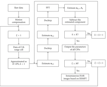
(c) Figure8: Instantaneous ISAR images based on the IHMPT.
100 200 300 400 500
Relative time 100
200
300
400
500
R
elati
ve
fr
equency
(a) 610th range bin
100 200 300 400 500
Relative time 100
200
300
400
500
R
elati
ve
fr
equency
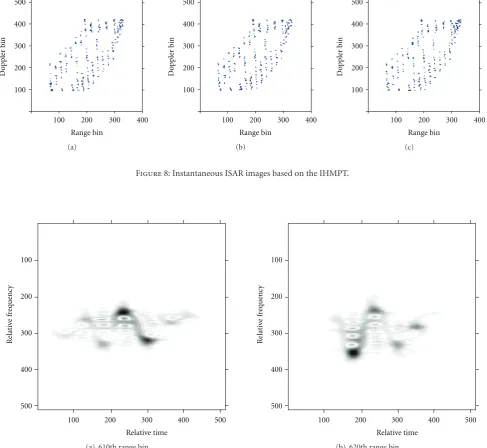
(b) 620th range bin Figure9: SPWVD of the received signal in a range bin.
whereqr,qp, andqy are the angular amplitudes in radians
and ωr,ωp, and ωy are the roll, pitch, and yaw angular
velocities, respectively.
The rotation parameters of the target are shown in Table 2, and the other parameters for the simulated data are
shown inTable 3.
The three-dimensional (3D) image of the target is shown inFigure 5.
We choose the received signal of the 1220th and 1251th range bins, and compute the smoothed pseudo-Wigner-Ville
distribution (SPWVD) of them, which are shown inFigure 6.
FromFigure 6, we can see that the time-varying character for the Doppler frequency is very complicated, and this demonstrates that the ship target has high maneuverability.
Figure 7is the ISAR image based on the RD algorithm. For the high maneuverability of the target, the image is blurred severely.
Figure 8 shows the instantaneous ISAR images at dif-ferent time positions based on the IHMPT algorithm; it is obvious that the image quality has been improved greatly.
5.2. Measured Data. We choose a set of measured data for
ship target to demonstrate the effectiveness of the IHMPT.
The radar works in the X band, and the radar parameters are not authorized to be published. The SPWVDs for the received signal in the 610th range bin and 620th range bin
are shown inFigure 9; it is obvious that the ship target has
200 400 600 500
1000
1500
2000
2500
Range bin
Do
p
p
le
r
b
in
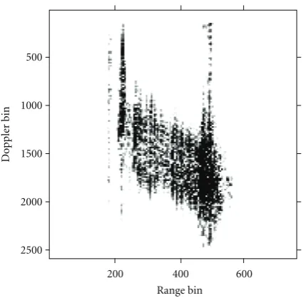
Figure10: ISAR image of ship target based on the RD algorithm.
500
400
300
200
100
Do
p
p
le
r
b
in
50 100 150
Range bin
(a)
500
400
300
200
100
Do
p
p
le
r
b
in
50 100 150
Range bin
(b)
500
400
300
200
100
Do
p
p
le
r
b
in
50 100 150
Range bin
(c)
Figure11: Instantaneous ISAR images based on the IHMPT.
Figure 10is the ISAR image based on the RD algorithm. For the high maneuverability of the target, the image is blurred severely.
The instantaneous ISAR images at different time
posi-tions based on the IHMPT algorithm are shown inFigure 11.
It is obvious that the quality has been improved greatly,
which demonstrates the effectiveness of the IHMPT
algo-rithm proposed.
6. Conclusion
For ISAR imaging of ship target with high maneuverability, the received signal in a range bin can be modeled as multicomponent cubic phase signal. The IHMPT can be used to estimate the parameters of the multicomponent cubic
phase signal, then combined with the RID technique, the high quality instantaneous ISAR images can be obtained.
Acknowledgments
References
[1] M. Martorella, “Novel approach for ISAR image cross-range scaling,”IEEE Transactions on Aerospace and Electronic Systems, vol. 44, no. 1, pp. 281–294, 2008.
[2] T. Thayaparan, L. J. Stankovic, C. Wernik, and M. Dakovic, “Real-time motion compensation, image formation and image enhancement of moving targets in ISAR and SAR using S-method-based approach,”IET Signal Processing, vol. 2, no. 3, pp. 247–264, 2008.
[3] M. Martorella and F. Berizzi, “Time windowing for highly focused ISAR image reconstruction,” IEEE Transactions on Aerospace and Electronic Systems, vol. 41, no. 3, pp. 992–1007, 2005.
[4] V. C. Chen and S. Qian, “Joint time-frequency transform for radar range-doppler imaging,”IEEE Transactions on Aerospace and Electronic Systems, vol. 34, no. 2, pp. 486–499, 1998. [5] V. Zeljkovic, Q. Li, R. Vincelette, C. Tameze, and F. Liu,
“Automatic algorithm for inverse synthetic aperture radar images recognition and classification,”IEE Proceedings Radar, Sonar and Navigation, vol. 4, no. 1, pp. 96–109, 2010. [6] M. Xing, R. Guo, C. W. Qiu, L. Liu, and Z. Bao,
“Experimen-tal research of unsupervised Cameron/maximum-likelihood classification method for fully polarimetric synthetic aperture radar data,”IEE Proceedings Radar, Sonar and Navigation, vol. 4, no. 1, pp. 85–95, 2010.
[7] S. K. Wong, G. Duff, and E. Riseborough, “Distortion in the inverse synthetic aperture radar (ISAR) images of a target with time-varying perturbed motion,”IEE Proceedings: Radar, Sonar and Navigation, vol. 150, no. 4, pp. 221–227, 2003. [8] F. Berizzi, E. D. Mese, M. Diani, and M. Martorella,
“High-resolution ISAR imaging of maneuvering targets by means of the range instantaneous Doppler technique: modeling and performance analysis,”IEEE Transactions on Image Processing, vol. 10, no. 12, pp. 1880–1890, 2001.
[9] T. Thayaparan, G. Lampropoulos, S. K. Wong, and E. Riseborough, “Application of adaptive joint time-frequency algorithm for focusing distorted ISAR images from simulated and measured radar data,”IEE Proceedings: Radar, Sonar and Navigation, vol. 150, no. 4, pp. 213–220, 2003.
[10] A. D. Lanterman, D. C. Munson, and Y. Wu, “Wide-angle radar imaging using time-frequency distributions,”IEE Pro-ceedings: Radar, Sonar and Navigation, vol. 150, no. 4, pp. 203– 211, 2003.
[11] Z. Bao, C. Sun, and M. Xing, “Time-frequency approaches to ISAR imaging of maneuvering targets and their limitations,”
IEEE Transactions on Aerospace and Electronic Systems, vol. 37, no. 3, pp. 1091–1099, 2001.
[12] G. Wang, Z. Bao, and X. Sun, “Inverse synthetic aperture radar imaging of nonuniformly rotating targets,” Optical Engineering, vol. 35, no. 10, pp. 3007–3011, 1996.
[13] J. Li and H. Ling, “Application of adaptive chirplet represen-tation for ISAR feature extraction from targets with rotating parts,”IEE Proceedings: Radar, Sonar and Navigation, vol. 150, no. 4, pp. 284–291, 2003.
[14] Y. Li, R. Wu, M. Xing, and Z. Bao, “Inverse synthetic aperture radar imaging of ship target with complex motion,”IET Radar, Sonar and Navigation, vol. 2, no. 6, pp. 395–403, 2008. [15] G. Zhao-Zhao, L. Ya-Chao, X. Meng-Dao, W. Genyuan, Z.
Shou-Hong, and B. Zheng, “ISAR imaging of manoeuvring targets with the range instantaneous chirp rate technique,”IET Radar, Sonar and Navigation, vol. 3, no. 5, pp. 449–460, 2009.
[16] Y. Wang and Y. Jiang, “ISAR imaging of a ship target using product high-order matched-phase transform,” IEEE Geoscience and Remote Sensing Letters, vol. 6, no. 4, Article ID 4785239, pp. 658–661, 2009.
[17] I. Djurovic, T. Thayaparan, and L. J. Stankovic, “Adaptive local polynomial Fourier transform in ISAR,”EURASIP Journal on Applied Signal Processing, Article ID 36093, 15 pages, 2006. [18] I. Djurovi´c, T. Thayaparan, and L. J. Stankovi´c, “SAR imaging
of moving targets using polynomial Fourier transform,”IET Signal Processing, vol. 2, no. 3, pp. 237–246, 2008.