Volume 2010, Article ID 438615,16pages doi:10.1155/2010/438615
Research Article
Subinteger Range-Bin Alignment Method for ISAR Imaging of
Noncooperative Targets
J. M. Mu˜
noz-Ferreras
1and F. P´erez-Mart´ınez
21Department of Signal Theory and Communications, Polytechnic School, University of Alcal´a, Campus Universitario,
Ctra. Madrid-Barcelona, Km. 33, 600, Alcal´a de Henares, 28805 Madrid, Spain
2Department of Signals, Systems and Radiocommunications, Technical University of Madrid, E.T.S.I. Telecomunicaci´on,
Avenida Complutense s/n, 28040 Madrid, Spain
Correspondence should be addressed to J. M. Mu˜noz-Ferreras,[email protected]
Received 17 November 2009; Accepted 25 March 2010
Academic Editor: Robert W. Ives
Copyright © 2010 J. M. Mu˜noz-Ferreras and F. P´erez-Mart´ınez. This is an open access article distributed under the Creative Commons Attribution License, which permits unrestricted use, distribution, and reproduction in any medium, provided the original work is properly cited.
Inverse Synthetic Aperture Radar (ISAR) is a coherent radar technique capable of generating images of noncooperative targets. ISAR may have better performance in adverse meteorological conditions than traditional imaging sensors. Unfortunately, ISAR images are usually blurred because of the relative motion between radar and target. To improve the quality of ISAR products, motion compensation is necessary. In this context, range-bin alignment is the first step for translational motion compensation. In this paper, we propose a subinteger range-bin alignment method based on envelope correlation and reference profiles. The technique, which makes use of a carefully designed optimization stage, is robust against noise, clutter, target scintillation, and error accumulation. It provides us with very fine translational motion compensation. Comparisons with state-of-the-art range-bin alignment methods are included and advantages of the proposal are highlighted. Simulated and live data from a high-resolution linear-frequency-modulated continuous-wave radar are included to perform the pertinent comparisons.
1. Introduction
Traditional imaging sensors, such as visible and infrared cameras or laser radar systems, may have a reduced performance in adverse weather conditions, like fog [1– 3]. Furthermore, in defense and security scenarios, smoke screens [4] may literally blind these imaging sensors based on very short wavelengths.
The origin of this degradation must be found in the extreme scattering that these wavelengths suffer when inter-acting with the little particles present in the atmosphere [1– 3]. When a high signal attenuation is present, the operation range of these sensors diminishes considerably.
However, in important applications related to defense and security, it is still necessary to obtain images for recogni-tion/identification purposes, regardless of the meteorological and scenario conditions.
Inverse Synthetic Aperture Radar (ISAR) is a coherent radar technique which may obtain images of noncooperative
targets [5, 6]. Furthermore, these images may be used for subsequent recognition tasks [7–10]. Although ISAR is usually understood as a complement for electro-optical sensors, it may in fact outperform these traditional sensors in adverse conditions, because it inherits the all-weather feature [11] from the long wavelength radars.
The standard scenario for ISAR consists of a static high-resolution coherent radar which illuminates a moving noncooperative target [12]. In this context, a noncooperative target is a target whose motion is unknown.
In ISAR, the two image dimensions are slant-range and Doppler (cross-range). High slant-range resolution is achieved by transmitting a large bandwidth signal, whereas high cross-range resolution depends on a large aspect angle variation of the target during the illumination time [12]. Specifically, the slant-range resolution is given by
ρr= c
where c is the light speed and Δf is the transmitted bandwidth. The cross-range resolution may be written as
ρa= λ
2Δθ, (2)
where λ is the transmitted wavelength and Δθ is the variation of the target aspect angle during the illumination (observation) time.
Target motion may be divided into a translational component and a rotational component [13,14]. The first one is further decomposed into a radial and a tangential component, whereas the second one has three attitude components: yaw, pitch, and roll.
On the one hand, the radial component of the transla-tional motion (i.e., the component along the line-of-sight (LOS)) is undesired, because it does not induce variation of the target aspect angle; that is, it does not generate Doppler gradient among target scatterers situated in the same range bin. Furthermore, this component causes a large blurring in ISAR images.
On the other hand, the rest of motion components may produce the desired Doppler gradient among scatterers, hence obtaining bidimensional information. It is true that the rotational motion (and the tangential component of the translational motion) may also generate blurring effects on the image [15], called Migration Through Resolution Cells (MTRCs), but these effects have minor importance in comparison to the large blurring generated by the radial component of the translational motion, which must always be compensated.
Methods for translational motion compensation work in two steps [16]: range-bin alignment and phase adjustment. For the first stage, which is the motivation of this paper, several methods may be found in the literature, such as the peak tracking approach [5], the centroid tracking algorithm [17], the envelope correlation method [5,18,19], the global range alignment approach [20], or the minimum-entropy-based technique [21]. For the second stage regarding phase adjustment, the literature provides us with famous methods such as prominent point processing [22], phase gradient autofocus [23], entropy minimization [16], or contrast maximization [24].
In this paper, we concentrate on the range-bin align-ment stage, which is fundaalign-mental to guarantee a proper translational motion compensation. Concretely, we present a subinteger range-bin alignment approach based on the traditional envelope correlation method and the use of reference profiles. This work was preliminarily presented in the conference paper [19]. Here, deep analyses as well as exhaustive comparisons with other existing methods both for simulated and live data are provided.
The proposed method makes use of reference profiles in order to mitigate the error accumulation phenomenon and the target scintillation effects [18], typical limitations of the earlier range-bin alignment approaches such as the peak and centroid tracking methods. Furthermore, the technique makes a subinteger alignment which provides us with a very fine range profile adjustment. This subinteger
10 12 14 16 18 20 22
1000 1100 1200 1300 1400 1500 1600 1700 1800 1900
τ
EC(
τ
)
Figure1: Envelope correlation (as a function of the range shiftτ) between a real shifted range profile and its corresponding reference profile.
TC
1/PRF
Δf
t f
f0 · · ·
Figure2: Waveform for an LFMCW radar.
alignment approach is based on an optimization stage which has carefully been designed in order to avoid possible convergence to local maxima.
The method is robust against noise, clutter, and target scintillation. Moreover, it properly solves the error accumu-lation problem. Its performance is similar to the state-of-the-art current methods such as the global range alignment approach [20] and the minimum entropy-based technique [21], although it provides two clear advantages; it properly solves extreme situations with large range shifts from pulse to pulse (unlike the global range alignment algorithm) and it has moreover the ability to produce subinteger fine range adjustments over a wide range of offsets (in contrast to the minimum entropy-based method).
Furthermore, the careful design of the method against local maxima makes it very robust, as shown here for controlled simulated examples for which the state-of-the-art methods have convergence problems.
0 5 10 15
R
elati
ve
heig
ht
(m)
−15 −10 −5 0 5 10 15 Length (m)
Figure3: Scatterer distribution for a simulated target illuminated by an LFMCW radar.
2. Subinteger Range-Bin Alignment Method
The proposed method uses the cross-correlation of range profiles in order to estimate the misalignment between them. The correlation is not calculated between the current range profile and the previous one, which would generate the undesired error accumulation effect [18]. On the contrary, the cross-correlation is calculated between the current range profile and a reference profile obtained as a combination of the previously aligned range profiles. This reduces the error accumulation effect and provides robustness against noise, clutter, and target scintillation. Moreover, the pro-posed alignment between the current and the reference profiles may be a fraction of one range bin, providing the method with a subinteger capability. This fine alignment is achieved after an optimization stage which has been designed to minimize possible convergence to local maxima. The following paragraphs describe the method.
Letpm(n) be themth acquired range profile, wheren=
0,. . .,N−1, m = 0,. . .,M−1, N is the total number of range bins andM is the number of acquired range profiles. Let us call pm(n) as the aligned profile of pm(n), after the
alignment process.
As previously commented, in order to reduce the error accumulation effect and to increase the method robustness against noise, clutter, and target scintillation, it is interesting to define a reference profile [18]. We calculate this reference profile as a combination of the previously aligned range profiles. Concretely, we follow the recommendations of [16] in order to define the reference profile rm+1(n) for the alignment ofpm+1(n) as
rm+1(n)= m
m+ 1rm(n) + 1
m+ 1pm(n), (3)
where rm(n) is the reference profile for the alignment of
the mth range profile pm(n). Note that the calculation of
rm+1(n) requires the knowledge of the previously aligned range profiles. This clearly demonstrates the iterative nature of the method.
Once the (m+1)th range profilepm+1(n) and its associ-ated reference profilerm+1(n) are available, the objective is to obtain the (m+1)th-aligned range profilepm+1(n). For this purpose, the envelope cross-correlation betweenrm+1(n) and a shifted version ofpm+1(n) is defined as
EC(τm+1)=
N−1
n=0
|rm+1(n)| ·pm+1(n−τm+1), (4)
whereτm+1 is the range shift applied to the (m+1)th range profilepm+1(n). The valueτm+1 is not necessarily an integer, so thatpm+1(n−τm+1) is calculated by using the shift property of the Fourier transform as follows:
pm+1(n−τm+1)=FFT
ej(2π/N)τm+1nIFFTp
m+1(n)
, (5)
wherenis the vector [0, 1,. . .,N−1]T.
In the context of this paper, a maximum value of the envelope correlation is indicative of an optimum alignment between the (m+1)th reference profile rm+1(n) and the shifted range profilepm+1(n−τm+1). Hence, we are interested in obtaining the optimum shift τm+1 that maximizes the envelope correlation. Mathematically, this optimum shift may be expressed as
τm+1=arg max
τm+1
EC(τm+1). (6)
After solving the optimization problem, we can finally obtain the aligned profilepm+1(n) as
pm+1(n)=pm+1(n−τm+1), (7)
where the range shift of the original profile is implemented by using (5), because this optimum shiftτm+1may be not an integer.
It is really interesting to analyze the optimization prob-lem expressed in (6) in order to visualize its nature.Figure 1 shows the value of the envelope correlation (see (4)) between a live-shifted range profile and its associated reference profile as a function of the shiftτ. In this example, the variableτis expressed in number of range bin.
The envelope correlation shown in Figure 1 shows a standard example which we have found typical for both simulated and real data. It can easily be seen that the objective cost function suffers from local maxima.
As a consequence, it is obvious that we have to pay great attention to the correct initialization of the optimization algorithm in order to guarantee the desired convergence to the global maximum. That is, if the initial guess for the optimization method is near to the global maximum, a correct convergence to it is achievable.
1020 1010 1000 990 980 970
Slant-r
ange
(m)
50 100 150 200 250
Number of range profile
0 −5 −10 −15 −20 −25 −30 −35 −40 −45 −50
(dB)
(a)
−80 −60 −40 −20 0 20 40 60 80 100 120
Do
p
p
le
r
(Hz)
980 990 1000 1010 1020 Slant-range (m)
0 −5 −10 −15 −20 −25 −30 −35 −40 −45 −50
(dB)
(b)
Figure4: (a) Range profiles and (b) ISAR image for the simulated example without radial translational velocity.
1020 1010 1000 990 980 970
Slant-r
ange
(m)
50 100 150 200 250
Number of range profile
0 −5 −10 −15 −20 −25 −30 −35 −40 −45 −50
(dB)
(a)
−240 −220 −200 −180 −160 −140 −120 −100 −80 −60 −40
Do
p
p
le
r
(Hz)
980 990 1000 1010 1020 Slant-range (m)
0 −5 −10 −15 −20 −25 −30 −35 −40 −45 −50
(dB)
(b)
Figure5: (a) Range profiles and (b) ISAR image for the simulated example with a radial translational velocity ofvr=10 m/s.
exhaustive procedures (like a grid method or a random walk).
Nevertheless, according to our observations of our avail-able simulated and real data, we have noticed that the peak corresponding to the global maximum of the cost function is quite wide, as seen inFigure 1. This means that a proper initial guess for the optimum shiftτm+1is simply the integer range shift for which the cross-correlation is maximum. Hence, we evaluate the cross-correlation for the possible integer shiftsn=0,. . .,N−1, and select the one for which the cost function is maximum as the initial guess for the subsequent standard optimization algorithm. This process lets us finally converge to the desired global maximum. In this paper, a zero-order optimization algorithm (the Nelder-Mead algorithm [25]) has been utilized to obtain the desired subinteger refinement forτm+1.
We would like to highlight that the commented method to obtain the initial guess properly worked in all the simulated and real data available to the authors. On the other hand, it is true that other optimization approaches, like a
gradient-based method or the Newton method, may have been used for the refinement stage. Our experience is that the zero-order Nelder-Mead algorithm worked properly for the analyzed examples.
As a summary, the following steps implement the pro-posed technique for ISAR subinteger range-bin alignment.
Step 1(m=0). Considerp0(n)=p0(n).
Step 2. Calculate the (m+1)th reference profilerm+1(n) using (3).
Step 3. Obtain the envelope correlation (see (4)) between
rm+1(n) and the (m+1)th-shifted range profile pm+1(n − τm+1), withτm+1being an integer in the interval [0, 1,. . .,N− 1] andNthe number of range bins.
1020 1010 1000 990 980 970
Slant-r
ange
(m)
50 100 150 200 250
Number of range profile
0 −5 −10 −15 −20 −25 −30 −35 −40 −45 −50
(dB)
Figure6: Range profiles for the simulated example after applying the peak tracking method. Note that the target scintillation phenomenon makes this approach fail.
Step 5. Solve (6) with the Nelder-Mead algorithm, taking
τm+1,0 as the initial guess for the iterative technique. As a result, obtain the optimum range shiftτm+1.
Step 6. Obtainpm+1(n) using (7). Use (5) if the optimum shiftτm+1is not an integer.
Step 7(m←m + 1). Ifm≤M−2, whereMis number of range profiles, go toStep 2to align the next range profile.
3. Simulation of an LFMCW Radar
In this section, we provide the tools to simulate targets illuminated by an LFMCW radar, because the simulated and real data used in this paper correspond to this type of radar. Next section will detail the properties of the proposed alignment method for this kind of data. Although the results detailed in the paper only refer to LFMCW radars, it is important to highlight that the proposed method is applicable to any coherent imaging radar.
An LFMCW radar transmits a continuous waveform whose instantaneous frequency as a function of the time is depicted in Figure 2. The central transmitted frequency is
f0, the pulse repetition frequency is PRF, the transmitted bandwidth is represented by Δf, whereas the parameter TC represents the necessary time for the radar circuits to
guarantee the signal coherence from ramp to ramp.
Next, we describe the radar signal model. The complex envelope of the transmitted signalsT(t) may be written as
sT(t)=exp j 2π f0t+πγt2
, (8)
wheret=t−mPRF−1,tis the time,mis the number of range profile (i.e., the number of ramp), and γis the chirp rate. Note that the received signal in the intervals corresponding toTCis not processed.
Table1: LFMCW radar parameters for the simulated example in
Figure 3.
Central frequency (f0) 10 GHz
Bandwidth (Δf) 500 MHz
Ramp Repetition Frequency (PRF) 500 Hz
TC 0.2 ms
Illumination Time (CPI) 0.5 s
If we consider a point-scatterer at a rangeRtk from the
radar, the received signal from the scatterer is
sRk(t)=σkexp
j
2π f0
t−2Rtk
c
+πγ
t−2Rtk
c
2
,
(9)
whereσkis a complex value associated to the scatterer, whose
amplitude represents the scatterer backscattering and the propagation losses, whereas its phase models a possible phase change inserted by the scatterer.
LFMCW radars usually apply hardware deramping, which consists of mixing the received signal with a replica of the transmitted signal. By considering that the target has Kscatterers, the beat signal after the deramping processing may be written as
sb(t)= K
k=1 σkexp
j
4πγRtk
c t+
4π f0 c Rtk−
4πγR2tk
c2
.
(10)
Note that, for each transmitted ramp, a range profile may be obtained. For an LFMCW radar, it is necessary to make a Fourier transform of the beat signal to obtain the range profiles. Effectively, by neglecting the last phase term in (10), it is clear that a Fourier transform in t supplies the range profile for each m. The beat frequency ftk for a scatterer
situated at a rangeRtkmay be written, from (10), as
ftk =
2γRtk
c . (11)
A correct sampling of (10) provides us with the possibility of simulating complex scenes. This is simply made by calculating the ranges from the radar to all target scatterers for all ramps. For each ramp, the corresponding range profile may be obtained by applying a Fourier transform to (10).
As an interesting example, let us consider the distribution of 2000 scatterers depicted inFigure 3. Let us say that these scatterers belong to a ship.
1020 1010 1000 990 980 970
Slant-r
ange
(m)
50 100 150 200 250
Number of range profile
0 −5 −10 −15 −20 −25 −30 −35 −40 −45 −50
(dB)
(a)
−240 −220 −200 −180 −160 −140 −120 −100 −80 −60 −40
Doppler
(Hz)
980 990 1000 1010 1020 Slant-range (m)
0 −5 −10 −15 −20 −25 −30 −35 −40 −45 −50
(dB)
(b)
Figure7: (a) Range profiles and (b) reconstructed ISAR image after applying the proposed subinteger range-bin alignment method to the simulated data with translational motion.
Figure8: Photo of the two-mast sailboat.
For this simulated example, we have considered that |σk| = 1, for allkand∠σkis uniformly distributed between
0 and 2π. Moreover, a signal-to-noise ratio of 10 dB has been considered, with the noise being additive, white, and Gaussian.
Figure 4(a)shows the 250 range profiles for this example, when the target is considered to have a radial translational speed of vr = 0 m/s. By applying an FFT in each range
bin, we obtain the ISAR image in the conventional range-Doppler coordinates (Figure 4(b)). In the context of this paper,Figure 4(b)must be considered as the optimum ISAR image for this simulation, because there is no blurring (i.e., the radial component of the translational motion is zero).
On the other hand, Figures5(a)and5(b), respectively, show the range profiles and the ISAR image for the previously simulated example, but considering that the target is moving away with a radial speed of vr = 10 m/s. The
leaning observed in the range profiles and the large blurring in the ISAR image are characteristic effects due to the radial component of the translational motion.
Because the dynamics for noncooperative targets are unknown, the objective of the blind motion compensation techniques consists of focusing the ISAR images without
additional information. For our simulated example, the blind techniques should obtain an image similar to Figure 4(b) from processing the data inFigure 5.
Next sections detail the performance of the proposed alignment algorithm in comparison with other existing methods for compensating the translational motion. In order to make fair comparisons among the diverse range-bin alignment techniques, in this paper we always use the method in [16] for the phase adjustment step.
4. Properties of the Proposed Method
This section addresses the performance of the proposed range-bin alignment technique in relation to important fea-tures: robustness against target scintillation, against clutter, and so forth. Both simulated and real data are used to verify the good performance of the proposed method.
4.1. Robustness against Target Scintillation. The signal received by the radar is the coherent sum of many contri-butions from target scatterers. This implies that the power in each range bin is not constant during the illumination time. This effect is known as target scintillation.
Target scintillation makes the standard tracking approaches fail. For example, Figure 6 shows the range profiles for our simulated example with a radial translational motion aligned after applying the peak tracking method. Clearly, the simulated data suffer from the target scintillation phenomenon, because we have simulated many point-scatterers. Target scintillation causes the location of the global maximum to strongly fluctuate between range profiles.
835 830 825 820 815 810
Slant-r
ange
(m)
50 100 150 200 250 300 350 400 Number of range profile
−5 −10 −15 −20 −25 −30 −35
(dB)
(a)
200 150 100 50 0 −50 −100 −150 −200
Do
p
p
le
r
(Hz)
810 815 820 825 830 835
Slant-range (m)
−5 −10 −15 −20 −25 −30 −35 Clutter
(dB)
(b)
Figure9: (a) Range profiles and (b) ISAR image for the real data of the two-mast sailboat. No motion compensation technique has been applied.
835 830 825 820 815 810
Slant-r
ange
(m)
50 100 150 200 250 300 350 400 Number of range profile
−5 −10 −15 −20 −25 −30 −35
(dB)
(a)
200 150 100 50 0 −50 −100 −150 −200
Do
p
p
le
r
(Hz)
810 815 820 825 830 835
Slant-range (m)
−5 −10 −15 −20 −25 −30 −35
(dB)
(b)
Figure10: (a) Range profiles and (b) ISAR image for the real data of the two-mast sailboat after applying the centroid tracking method.
835 830 825 820 815 810
Slant-r
ange
(m)
50 100 150 200 250 300 350 400 Number of range profile
−5 −10 −15 −20 −25 −30 −35
(dB)
(a)
200 150 100 50 0 −50 −100 −150 −200
Do
p
p
le
r
(Hz)
810 815 820 825 830 835
Slant-range (m)
−5 −10 −15 −20 −25 −30 −35
(dB)
(b)
1020 1010 1000 990 980 970
Slant-r
ange
(m)
50 100 150 200 250
Number of range profile
0 −5 −10 −15 −20 −25 −30 −35 −40 −45 −50
(dB)
(a)
−240 −220 −200 −180 −160 −140 −120 −100 −80 −60 −40
Do
p
p
le
r
(Hz)
980 990 1000 1010 1020 Slant-range (m)
0 −5 −10 −15 −20 −25 −30 −35 −40 −45 −50
(dB)
(b)
Figure12: (a) Range profiles and (b) ISAR image without using reference profiles. The results correspond to the simulated data presented inFigure 5.
Figure13: Photo of the vessel.
be seen that a proper range-bin alignment has been obtained. In fact, this result is very similar to the range profiles shown in Figure 4(a), which may be understood as the optimum range profiles, because they correspond to the simulated example without translational motion.
Figure 7(b)shows the motion-compensated ISAR image obtained with the proposed technique for the range-bin alignment stage and with the method in [16] for the phase adjustment stage. Hence, Figure 7(b) is the reconstructed ISAR image after using the proposed technique. Note that this reconstruction is a very good approximation to the optimum ISAR image shown inFigure 4(b).
4.2. Robustness against Noise and Clutter. Thermal noise is always present in real systems. The simulated examples shown in this paper include thermal noise. On the other hand, clutter may exist depending on the acquisition sce-nario. For example, in maritime scenarios, the clutter due to echoes from the sea may be a problem.
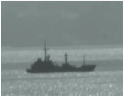
Figure 8shows the photograph of a noncooperative two-mast sailboat, which was illuminated during an acquisition
Table2: Real radar parameters for the acquired data corresponding to the sailboat inFigure 8.
Central frequency (f0) 28.5 GHz
Bandwidth (Δf) 1 GHz
Ramp repetition frequency (PRF) 1000 Hz
TC 0.1 ms
Illumination time (CPI) 0.4 s
campaign made in the Strait of Gibraltar. The circles approximately indicate the positions of the mast bases and tips and the sailboat bow and stern. The real radar [26] is a high-resolution millimeter-wave LFMCW radar, whose parameters for this acquisition are detailed inTable 2.
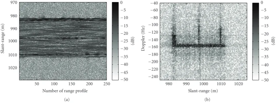
This live example is an interesting one, since the sea state was 4 and many clutter echoes were received. Figures 9(a)and9(b), respectively, show the range profiles and the ISAR image for this capture without applying any motion compensation technique. We can see that the signal-to-noise ratio is poor and that energetic echoes corresponding to clutter are evident. Moreover, the ISAR image is blurred because of the translational motion of the target, which is evident from the characteristic leaning observed in the range profiles in Figure 9(a). Certainly, it is difficult to distinguish the details of the ship in the ISAR image shown inFigure 9(b).
7040 7030 7020 7010 7000 6990 6980 6970
Slant-r
ange
(m)
100 200 300 400 500 600 Number of range profile
−5 −10 −15 −20 −25 −30 −35
(dB)
(a)
240 220 200 180 160 140 120 100 80
Do
p
p
le
r
(Hz)
6970 6980 6990 7000 7010 7020 7030 7040 Slant-range (m)
−5 −10 −15 −20 −25 −30 −35
(dB)
(b)
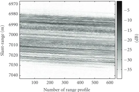
Figure14: (a) Range profiles and (b) ISAR image for the real data of the vessel without compensating the translational motion.
7040 7030 7020 7010 7000 6990 6980 6970
Slant-r
ange
(m)
100 200 300 400 500 600 Number of range profile
−5 −10 −15 −20 −25 −30 −35
(dB)
(a)
240 220 200 180 160 140 120 100 80
Do
p
p
le
r
(Hz)
6970 6980 6990 7000 7010 7020 7030 7040 Slant-range (m)
−5 −10 −15 −20 −25 −30 −35
(dB)
(b)
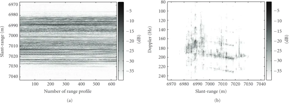
Figure15: (a) Range profiles and (b) ISAR image for the real data of the vessel after applying the proposed method.
Certainly, the high levels of noise and clutter for this example make the tracking-based methods fail.
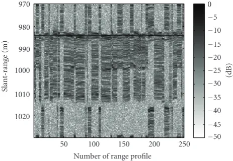
On the other hand,Figure 11(a)presents the range pro-files aligned by the proposed subinteger range-bin alignment method. In this case, we can see that the range profiles are more properly aligned.Figure 11(b)shows the reconstructed ISAR image for this case, where the masts and the deck are more detailed in comparison to Figures9(b)and10(b).
Hence, the proposed range-bin alignment method is robust against high levels of noise and clutter. So far, the drawn conclusions are based on visual inspection. However, we can use focusing indicators to quantify the quality improvement observed in the ISAR image ofFigure 11(b). In this context and for this kind of examples, we can use the entropy [16] and the contrast [24], whose mathematical definitions are given in the corresponding references. The lower the entropy, the more focused the ISAR image is [16]. And, the greater the contrast, the more focused the ISAR image is [24].
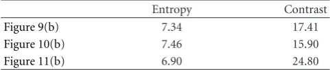
These focusing indicators for the ISAR images of Figures 9(b),10(b), and11(b)are detailed inTable 3. According to these results, we have that the ISAR image after applying the
Table3: Focusing indicators for the live ISAR images in Figures
9(b),10(b), and11(b).
Entropy Contrast
Figure 9(b) 7.34 17.41
Figure 10(b) 7.46 15.90
Figure 11(b) 6.90 24.80
proposed technique is more focused than the original image without compensating the translational motion and is also more focused than the image obtained with the tracking-based range-bin alignment approach. We even obtain that the quality of the ISAR image after applying the centroid tracking technique gets worse in relation toFigure 9(b).
7040 7030 7020 7010 7000 6990 6980 6970
Slant-r
ange
(m)
100 200 300 400 500 600 Number of range profile
−5 −10 −15 −20 −25 −30 −35
(dB)
(a)
240 220 200 180 160 140 120 100 80
Doppler
(Hz)
6970 6980 6990 7000 7010 7020 7030 7040 Slant-range (m)
−5 −10 −15 −20 −25 −30 −35
(dB)
(b)
Figure16: (a) Range profiles and (b) ISAR image for the real data of the vessel after using the global range alignment algorithm.
7040 7030 7020 7010 7000 6990 6980 6970
Slant-r
ange
(m)
100 200 300 400 500 600 Number of range profile
−5 −10 −15 −20 −25 −30 −35
(dB)
Figure17: Range profiles of the vessel with an artificially induced vibration.
For example, for envelope correlation-based methods, the error accumulation effect takes importance when the alignment of the current range profile is only based on the previously aligned range profile, as shown next.
Figure 12(a)shows the range profiles obtained after using a reduced version [5] of the proposed method for aligning the range profiles of the simulated example inFigure 5. This simplified algorithm defines the reference profile rm+1(n) for the alignment of the (m+1)th range profile pm+1(n) as the previously aligned range profile, that is, rm+1(n) =
pm(n), according to the nomenclature used in Section 2.
In Figure 12(a), some misalignment error accumulates, as clearly shown if we concentrate, for example, on the range history for the scatterers on sailboat stern. These range variations are not observed inFigure 7(a).
The error accumulation effect inFigure 12(a)has minor incidence on the results ofFigure 7(a). Hence, the proposed range-bin alignment method based on the use of reference profiles is robust against this phenomenon.
On the other hand,Figure 12(b)shows the ISAR image obtained from the range profiles in Figure 12(a). This image is defocused in comparison with the ISAR image in
Table 4: Focusing indicators for the simulated ISAR images in Figures7(b)and12(b).
Entropy Contrast
Figure 7(b) 7.17 10.60
Figure 12(b) 7.81 8.97
Figure 7(b). This is obvious for the scatterers on the sailboat deck, for example. In fact, the same may be concluded if we calculate the focusing indicators for Figures7(b)and12(b), asTable 4details.
5. Comparison with State-of-the-Art Methods
In previous section, we exposed the properties of the proposed alignment method by using both simulated and real data. Here, it is our intention to compare the proposed approach with state-of-the-art methods recently proposed in the literature: concretely, the global range alignment algorithm [20] and the minimum entropy-based approach [21].
The performance of the proposed subinteger range-bin alignment technique is similar to the one for these state-of-the-art methods, as shown next. However, the proposed approach can deal with extreme situations with large-range shifts from range profile to range profile. Moreover, its subinteger alignment capability is also noticeable and, unlike the other methods, the careful design of the optimization stage increases its robustness against possible convergence to local maxima.
To make the pertinent comparisons, we use the live data described in the following. Figure 13 shows the photo of a vessel illuminated by the millimeter-wave LFMCW radar prototype [26]. The radar parameters for this acquisition are detailed inTable 5.
7040 7030 7020 7010 7000 6990 6980 6970
Slant-r
ange
(m)
100 200 300 400 500 600 Number of range profile
−5 −10 −15 −20 −25 −30 −35
(dB)
(a)
7040 7030 7020 7010 7000 6990 6980 6970
Slant-r
ange
(m)
100 200 300 400 500 600 Number of range profile
−5 −10 −15 −20 −25 −30 −35
(dB)
(b)
Figure18: Range profiles aligned after applying (a) the proposed subinteger range-bin alignment method and (b) the global range alignment algorithm to the vessel data with artificially induced vibration.
240 220 200 180 160 140 120 100 80
Do
p
p
le
r
(Hz)
6970 6980 6990 7000 7010 7020 7030 7040 Slant-range (m)
−5 −10 −15 −20 −25 −30 −35
(dB)
(a)
240 220 200 180 160 140 120 100 80
Do
p
p
le
r
(Hz)
6970 6980 6990 7000 7010 7020 7030 7040 Slant-range (m)
−5 −10 −15 −20 −25 −30 −35
(dB)
(b)
Figure19: ISAR images obtained after applying (a) the proposed subinteger range-bin alignment method and (b) the global range alignment algorithm to the vessel data with artificially induced vibration.
a
b
c d
a
b c
d
(a)
a b c d
a b c
d
(b)
a b c d
a b c d
(c)
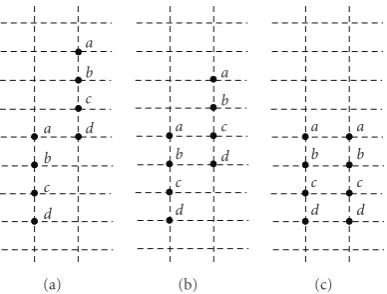
Figure20: Alignment process of two range profiles for the global range alignment algorithm.
is largely blurred because of the radial component of the translational motion, which can easily be guessed from the leaning observed in the range profiles ofFigure 14(a).
Table5: Real radar parameters for the acquired data corresponding to the vessel inFigure 13.
Central frequency (f0) 28.5 GHz
Bandwidth (Δf) 1 GHz
Ramp repetition frequency (PRF) 500 Hz
TC 0.2 ms
Illumination time (CPI) 1.27 s
Figure 15 presents the aligned range profiles and the focused ISAR image after applying the proposed subinteger range-bin alignment method and the method in [16] for the phase adjustment stage. Note the increase in the ISAR image quality. The masts and the deck appear focused. Certainly, the alignment produced by the proposed method seems to be good.
5 10 15 20 25 30 35 40
N
u
mber
of
ra
nge
b
in
1 2
Number of range profile
2.5
2
1.5
1
0.5
(a)
5 10 15 20 25 30 35 40
N
u
mber
of
ra
nge
b
in
1 2
Number of range profile
2.5
2
1.5
1
0.5
(b)
Figure21: Alignment results for two simulated range profiles by applying (a) the proposed technique and (b) the global range alignment algorithm. The proposed method is robust against local maxima of its cost function. On the contrary, the global range alignment method may have convergence difficulties.
7040 7030 7020 7010 7000 6990 6980 6970
Slant-r
ange
(m)
100 200 300 400 500 600 Number of range profile
−5 −10 −15 −20 −25 −30 −35
(dB)
(a)
240 220 200 180 160 140 120 100 80
Do
p
p
le
r
(Hz)
6970 6980 6990 7000 7010 7020 7030 7040 Slant-range (m)
−5 −10 −15 −20 −25 −30 −35
(dB)
(b)
Figure22: (a) Range profiles and (b) ISAR image for the real data of the vessel after using the minimum entropy-based approach.
Table6: Focusing indicators for the real ISAR images of the vessel in Figures14(b)and15(b).
Entropy Contrast
Figure 14(b) 9.32 8.7
Figure 15(b) 7.37 39.8
5.1. Comparison with the Global Range Alignment Algorithm. The global range alignment method [20] is also a robust method which usually performs well in diverse scenarios. As a proof of that, Figures 16(a) and 16(b), respectively,
show the range profiles and the ISAR image for the nonco-operative data ofFigure 14after applying this global range alignment approach. Figure 16(b) is practically indistin-guishable from the one obtained by the proposed approach (Figure 15(b)).
Hence, the global range alignment algorithm provides a good alignment. In fact, the focusing indicators for Figure 16(b)are almost the same as the ones forFigure 15(b). The entropy and contrast forFigure 16(b)are 7.36 and 39.9, respectively.
7020 7019 7018 7017 7016 7015 7014 7013
Slant-r
ange
(m)
80 100 120 140 160 180 200 220 240 260 Number of range profile
−5 −10 −15 −20 −25 −30 −35
(dB)
Figure23: Zoom ofFigure 22(a). The jumps in the range profiles are clearly visible.
a
b
a
b
Figure24: Two simple misaligned range profiles with little target scintillation.
arise, the global range alignment algorithm may fail, as also indicated in [21].
As a proof of that, let us concentrate onFigure 17, which shows the range profiles of the vessel with an artificially induced vibration. To simulate this vibration, each range profile has independently been shifted, with the shift being a Gaussian random variable of zero mean and a standard deviation of 10 cm. This has let us simulate a large vibration. Figure 18presents the results provided by the proposed and the global range alignment methods for the range profiles shown inFigure 17. By analyzingFigure 18, we can conclude that the proposed technique is robust against large range displacements, whereas the global range alignment algorithm cannot properly solve these situations.
It is obvious that the poor performance of the global range alignment method shown inFigure 18(b)has influence on the subsequent obtained ISAR image.Figure 19shows the ISAR images obtained after applying the proposed method and the global range alignment algorithm to the vessel data with artificially induced vibration. Again, the technique in [16] has been used for the phase adjustment step. Because of the misalignment, the ISAR image after the global range alignment approach is blurred. On the contrary, the ISAR
image obtained with the proposed technique is very similar to the one given inFigure 15(b).
On the other hand, it is noticeable that the optimization stage in the proposed technique has carefully been designed. On the contrary, the global range alignment method may have difficulties with local maxima of its cost function C
[20, equation (8)]. To visualize this, let us consider two single misaligned range profiles, as Figure 20(a) indicates. The parametersa,b,c,anddare the absolute values of the echoes in the corresponding range bins. An intermediate step in the optimization process of the global range alignment method is depicted in Figure 20(b). Figure 20(c) indicates the correct alignment of the two range profiles.
It can easily be shown that the values ofCin the situation depicted in Figures20(a)and20(b)are, respectively,
C(a)=2a2+b2+c2+d2+ad, C(b)=2
a2+b2+c2+d2+ac+db.
(12)
From the optimization algorithm given in [20], if C(a) > C(b), that is, if ad > ac + db, then the global range alignment algorithm will not converge to the correct result in Figure 20(c). Instead of that, it will try to refine the situation inFigure 20(a). As a proof of this fact,Figure 21shows the two range profiles aligned after using the proposed method and the global range alignment algorithm, whena=3,b= 0.25,c=0.5, andd=1. The global range alignment method is clearly affected by the local maximum and does not converge to the situation inFigure 20(c). On the contrary, the proposed method can deal with these cases because of the careful design of its optimization stage.
5.2. Comparison with the Minimum Entropy-Based Approach. The minimum entropy-based approach [21] for range-bin alignment is an iterative approach which is based on integer shifts of the range profiles, unlike the proposed method and the global range alignment algorithm.
Figure 22(a) shows the range profiles obtained after applying the entropy-based method to the real data of the vessel in Figure 14. Figure 22(b) shows the corresponding ISAR image.
Apparently, the range profiles shown in Figure 22(a) seem to be properly aligned. However, the fact that the range profiles may only be shifted in integer steps implies that undesired jumps occur in the range history of the target scatterers.Figure 23presents a zoom ofFigure 22(a)which allows distinguishing the commented jumps. Some of them are marked with an arrow.
These discontinuities appearing in the range profiles induce an amplitude modulation in Doppler. This is the rea-son why spurious images are clearly visible inFigure 22(b). Hence, the ISAR image obtained with the minimum entropy-based approach has a quality poorer than the one in Figure 15(b). The entropy and contrast for the ISAR image inFigure 22(b)(8.01 and 35.3, resp.) are also indicative of this quality decrease. Please refer toTable 6.
2 4 6 8 10 12
N
u
mber
of
ra
nge
b
in
1 2
Number of range profile
3
2.5
2
1.5
1
0.5
(a)
2 4 6 8 10 12
N
u
mber
of
ra
nge
b
in
1 2
Number of range profile
3
2.5
2
1.5
1
0.5
(b)
Figure25: Alignment results for the two simulated range profiles inFigure 24by applying (a) the proposed technique and (b) the minimum entropy-based approach.
range-bin alignments. This has been done in a way similar to the optimization stage given in the proposed method. Unfortunately, the commented jumps still appear when applying this extension.
On the other hand, the minimum entropy-based approach may also have problems with local maxima. As a proof of that, let us consider two misaligned range profiles as shown inFigure 24. The valuesa,a,b,andbare the absolute values of the echoes in the corresponding range bins. Let us also assume that we have a little target scintillation, in such a way that we assumea≈aandb≈b.
From the equations given in [21], it can easily be shown that the minimum entropy-based method will not be able to align the two range profiles inFigure 24, if the next two conditions are met:
alna+blnb > alna+blnb,
alna+blnb> alna+blnb.
(13)
Let us consider thata=3.1,b=1,a=3, andb=1.1. These values satisfy (13).Figure 25(b)shows the two range profiles after applying the minimum entropy-based approach for this case. As predicted, the method is unable to align the two range profiles. On the contrary, the proposed method can align the two range profiles, as shown inFigure 25(a). Again, we would like to highlight that the optimization stage of the proposed method has carefully been designed.
6. Conclusions
The traditional imaging sensors, such as cameras or laser radars, may have a reduced performance in adverse mete-orological conditions or in difficult scenarios where, for example, smoke screens are present. ISAR is an all-weather radar technique which may provide images of noncoop-erative targets in such adverse environments. Hence, such images are interesting for defense and security applications. Furthermore, the ISAR images may be exploited for subse-quent recognition/identification tasks.
Unfortunately, the standard ISAR images are usually blurred because of the target motion. Motion compensation techniques should be applied in order to have focused ISAR images. Generally, it is at least necessary to compensate the radial component of the translational motion. To achieve this, the methods for translational motion compensation work in two stages: range-bin alignment and phase adjust-ment.
The paper addresses the performance of the proposed algorithm in an exhaustive manner, by using both simulated and real data from LFMCW radars. In this context, it has been shown that the method is robust against target scintillation, noise, and clutter. Its robustness against the error accumulation effect has also been verified.
On the other hand, the proposed method has also been compared with recently proposed state-of-the-art range-bin alignment methods, such as the global range alignment algorithm and the minimum entropy-based approach. We have verified that the subinteger feature of the proposed method provides us with extremely accurate range-bin alignments, in contrast to the minimum entropy-based approach. It has also been shown that the method may deal with large range shifts from range profile to range profile, unlike the global range alignment algorithm. Finally, the careful design of the proposed optimization stage has been highlighted. We have addressed simple simulated examples in which both the global range alignment algorithm and the minimum entropy-based technique have problems with local maxima.
The proposed algorithm is robust in many scenarios and is hence a very interesting alternative for the range-bin alignment stage in the task of ISAR translational motion compensation. The improved obtained ISAR images may be of interest for subsequent automatic target recognition methods.
Acknowledgments
This work was financially supported by the Spanish National Board of Scientific and Technology Research under Project TEC2008-02148/TEC. The authors thank Dr. A. Blanco-del-Campo, Dr. A. Asensio-L ´opez, and Dr. B. P. Dorta-Naranjo for providing the live data of the sailboat and the vessel.
References
[1] S. A. Hovanessian, Introduction to Sensor Systems, Artech House, Boston, Mass, USA, 1988.
[2] A. V. Jelalian, Laser Radar Systems, Artech House, Boston, Mass, USA, 1992.
[3] G. R. Osche and D. S. Young, “Imaging laser radar in the near and far infrared,”Proceedings of the IEEE, vol. 84, no. 2, pp. 103–125, 1996.
[4] H.-Y. Chen, I.-Y. Tarn, and Y.-J. Hwang, “Infrared extinction of the powder of brass 70Cu/30Zn calculated by the FDTD and turning bands methods,”IEEE Transactions on Geoscience and Remote Sensing, vol. 33, no. 6, pp. 1321–1324, 1995.
[5] C.-C. Chen and H. C. Andrews, “Target motion induced radar imaging,”IEEE Transactions on Aerospace and Electronic Systems, vol. 16, no. 1, pp. 2–14, 1980.
[6] D. A. Ausherman, A. Kozma, J. L. Walker, H. M. Jones, and E. C. Poggio, “Developments in radar imaging,” IEEE Transactions on Aerospace and Electronic Systems, vol. 20, no. 4, pp. 363–400, 1984.
[7] K.-T. Kim, D.-K. Seo, and H.-T. Kim, “Efficient classification of ISAR images,”IEEE Transactions on Antennas and Propaga-tion, vol. 53, no. 5, pp. 1611–1621, 2005.
[8] B. K. Shreyamsha Kumar, B. Prabhakar, K. Suryanarayana, V. Thilagavathi, and R. Rajagopal, “Target identification using harmonic wavelet based ISAR imaging,”EURASIP Journal on Applied Signal Processing, vol. 2006, Article ID 86053, 13 pages, 2006.
[9] E. Radoi, A. Quinquis, and F. Totir, “Supervised self-organizing classification of superresolution ISAR images: an anechoic chamber experiment,”EURASIP Journal on Applied Signal Processing, vol. 2006, Article ID 35043, 14 pages, 2006. [10] S. Musman, D. Kerr, and C. Bachmann, “Automatic
recogni-tion of ISAR ship images,”IEEE Transactions on Aerospace and Electronic Systems, vol. 32, no. 4, pp. 1392–1404, 1996. [11] M. I. Skolnik, Introduction to Radar Systems, McGraw Hill
Higher Education, McGraw Hill, New York, NY, USA, 3rd edition, 2001.
[12] D. R. Wehner,High Resolution Radar, Artech House, Boston, Mass, USA, 2nd edition, 1995.
[13] V. C. Chen and W. J. Miceli, “Simulation of ISAR imaging of moving targets,”IEE Proceedings: Radar, Sonar and Navigation, vol. 148, no. 3, pp. 160–166, 2001.
[14] V. C. Chen,Time-Frequency Transforms for Radar Imaging and Signal Analysis, Artech House, Boston, Mass, USA, 2002. [15] J. L. Walker, “Range-Doppler imaging of rotating objects,”
IEEE Transactions on Aerospace and Electronic Systems, vol. 16, no. 1, pp. 23–52, 1980.
[16] L. I. Xi, G. Liu, and N. Jinlin, “Autofocusing of ISAR images based on entropy minimization,”IEEE Transactions on Aerospace and Electronic Systems, vol. 35, no. 4, pp. 1240–1252, 1999.
[17] J. M. Mu˜noz-Ferreras, J. Calvo-Gallego, F. P´erez-Mart´ınez, A. Blanco-del-Campo, A. Asensio-L ´opez, and B. P. Dorta-Naranjo, “Motion compensation for ISAR based on the shift-and-convolution algorithm,” inProceedings of the IEEE Conference on Radar, pp. 366–370, Verona, NY, USA, April 2006.
[18] G. Y. Delisle and H. Wu, “Moving target imaging and trajectory computation using ISAR,” IEEE Transactions on Aerospace and Electronic Systems, vol. 30, no. 3, pp. 887–899, 1994.
[19] J. M. Mu˜noz-Ferreras and F. P´erez-Mart´ınez, “Extended envelope correlation for range bin alignment in ISAR,” in
Proceedings of the IET International Conference on Radar Systems, pp. 65–68, Edinburg, UK, October 2007.
[20] J. Wang and D. Kasilingam, “Global range alignment for ISAR,”IEEE Transactions on Aerospace and Electronic Systems, vol. 39, no. 1, pp. 351–357, 2003.
[21] D. Zhu, L. Wang, Y. Yu, Q. Tao, and Z. Zhu, “Robust ISAR range alignment via minimizing the entropy of the average range profile,”IEEE Geoscience and Remote Sensing Letters, vol. 6, no. 2, pp. 204–208, 2009.
[22] B. D. Steinberg, “Microwave imaging of aircraft,”Proceedings of the IEEE, vol. 76, no. 12, pp. 1578–1592, 1988.
[23] D. E. Wahl, P. H. Eichel, D. C. Ghiglia, and C. V. Jakowatz Jr., “Phase gradient autofocus—a robust tool for high resolution SAR phase correction,”IEEE Transactions on Aerospace and Electronic Systems, vol. 30, no. 3, pp. 827–835, 1994.
[25] J. A. Nelder and R. Mead, “A simplex method for function minimization,” The Computer Journal, vol. 7, pp. 308–313, 1965.