ISSN 2286-4822 www.euacademic.org
Impact Factor: 3.4546 (UIF) DRJI Value: 5.9 (B+)
Parametric Bootstrap Method of Gini Index
Analysis in Gamma Distribution: A Diagnostic
Approach
EHTESHAM HUSSAIN
Department of Statistics, University of Karachi, Pakistan
MUHAMMAD AHSANUDDIN
Department of Economics, University of Karachi, Pakistan
MASOOD UL HAQ
Usman Institute of Technology, Karachi, Pakistan
Abstract
The Gini index is commonly used in the analysis of income distribution, and it is determined that the Gamma distribution, in many situations fits family income better than the other statistical distribution. However, Gini index in the Gamma distribution has its complex form, and its exact sampling distribution is hard to obtain. An alternative to this problem is Bootstrap method which makes enormous use of the computer’s ability to get to the solution. In this piece of research, the sampling properties of Gini index in Gamma distribution are investigated. The study utilizes simple random sampling (SRS) with replacement. The sample sizes used were n = 5, 10, 20 and 200, and all the simulations were based on 500 replicates. Consistent estimates were acquired with negligible error of ̂ and was found
that ̂is slightly biased for smaller size samples but it decreases as the
sample size increases.
Key words:Bootstrap, Gamma distribution, Gini index, Simple
random sampling
1. INTRODUTION
compute the equality of opportunity (Weymark, 2003; Kovacevic, 2010; Roemer, 2013; Brunori et al., 2013), assess economic inequality as well to determine income mobility (Khor and Pencavel, 2008; Macheras, 2016). Similarly, the Gamma distribution has also been considered as the model for the distribution of income (McDonald and Jensen, 1979; Chakraborti and Patriarca, 2008; Mori et al., 2015). However, Gini index in the Gamma distribution has its complex form, and its exact sampling distribution is tedious to obtain in normal circumstances. Hence, a practical way to improve upon first-order approximations is to apply bootstrap technique that makes possible difficult calculations necessary for analysis (Singh and Xie, 2008; Dodge, 2012). In this study sampling behavior of Gini index from Gamma distribution is considered by utilizing bootstrap method using Mathematica (Wolfram, 1991) for computational analysis.
1.1 The Gamma distribution
A gamma distribution is common type of statistical distribution that is right-skewed and continuous. It is related to the beta distribution and arises logically in processes for which the coming up times between Poisson distributed events are related. Gamma distribution are often employed in real-life situations that has a natural minimum of zero.
The Gamma distribution with parameter α > 0, β > 0, has density function
( ) ( )
y > 0 (1)
where α is a shape parameter and is scale parameter. is a
gamma function. The Gamma distributions are positively skewed, though the skewness tends to zero for large α.
The Gini index is given by ½ of ratio of Gini’s Mean Difference (GMD) to its mean
| | (2)
( ) (3)
| |
(4)
The Gini index is a commonly used measure of income inequality that condenses the entire income distribution for a country into a single number between 0 and 1; the higher the number, the greater the degree of income inequality.
Its natural estimator is given by
∑ ∑ | |
̅ (6)
In case of gamma distribution Gini index is given by
( ) ( )
( ) (7)
where µ = α/β denotes the mean of X.
If G = 0, income is perfectly equally distributed; G = 0.5, income is semi-unequally distributed, G = 1.0, income completely unequally distributed. The β is simply a scale factor hence G is invariant with respect to changes in β.
Table-I shows computed values of Gini index in case of gamma distribution for some specific values of α.
Table-I. Gini index ( )with reference to gamma distribution. α 1.0 1.5 2.0 2.5 3.0 3.5 4.0 4.5 5.0
( ) 0.5 0.42443 0.37500 0.339531 0.3215 0.291036 0.273438 0.25869 0.246094
Fig.1. Relation between α and ( )
Fig.1 shows relation between α and ( ) which reveals that for
large values of α, ( ) tends to zero and income is equally
2. EXACT SAMPLING DISTRIBUTION
Due to mathematical complexity precise sampling distribution is difficult to determine. As an alternative method this investigation uses bootstrap simulation. The bootstrap may also be used to obtain confidence intervals for the true parameter-values. The bootstrap makes vast use of the computer’s ability to carry out speedily routine and repetitive calculations.
2.1 Estimation
The method of moments estimators (MME) of α and β are defined by
̅ ̂̂ , ̂̂ (8)
with corresponding Maximum Likelihood Estimator (MLE) defined by
̅ ̂̃ and ( ̅
̃) ( ̂) ( ̂) (9)
where ̅ and ̃ denote the sample arithmetic and geometric
means respectively and represents the sample variance, and
(.) is digamma function. MLE of G is obtained by substituting α into (7). Estimation of α by (9) is time consuming and a better approximate expression is demonstrated by Johnson et al. (1995).
̂ ̃ ( )
(0 < Y ≤ 0.5772) (10)
̂ ̃ ( ) ( )
(0.57772 ≤ Y ≤ 17) (11) where Y = log arithmetic mean
geometric mean
The error of (10) does not exceed 0.0088% and that of (11) does not exceed 0.0054%.
3. BOOTSTRAP STUDY OF THE SAMPLING
DISTIBUTION
To demonstrate the performance of the Gini index estimator ̂ a
Setp1: using known pdf form as in (1);
Step2: Specify parameters values ;
Step3: Generate a random sample from of size n; Step4: Estimate MLE of parameters ̃ ̃;
Step5: Estimate MLE of ̂( ̃) as in (8);
Step6: Record the value of ̂( ̂);
Step7: Switch parameters in Step:2 by Step 4; Step 8: Repeat steps 2 to 6 B times;
Step9: Compute ( ̂( ̂)) ∑ ̂( ̂) and√ ( ̂( ̂)) . 3.1 Point Estimate
Estimate of ̂, based on 500 replicates are given in table-II (a,
b, c, and d) for the samples (n = 5, 10, 20, 200) taken from the Gamma distributions for (α = 2.5, 3, 3.5 and 4).
Table-II a α = 2.5
G(α) = 0.3395
n 5 10 20 200
( ̂) 0.2483 0.2810 0.2900 0.2981
Bias 0.0912 0.0585 0.0495 0.0414
√ ( ̂) 0.0817 0.0618 0.0438 0.0126
Table-II b α = 3
G(α) = 0.3125
n 5 10 20 200
( ̂) 0.2276 0.2580 0.2665 0.2735
Bias 0.0849 0.0545 0.0460 0.039
√ ( ̂) 0.0760 0.0574 0.0399 0.0118
Table-II c α = 3.5
G(α) = 0.2910
n 5 10 20 200
( ̂) 0.2139 0.2379 0.2468 0.2553
Bias 0.0772 0.0531 0.0442 0.0357
√ ( ̂) 0.0749 0.0488 0.0383 0.0118
Table-II d α = 4
G(α) = 0.2734
n 5 10 20 200
( ̂) 0.2009 0.2217 0.2317 0.2381
Bias 0.0725 0.0517 0.0417 0.0357
In the same tables also given standard deviations √ ( ̂) among
500 replicated estimates of G, which shows that, ̂ is slightly
bias, bias reduces as the sample size increases.
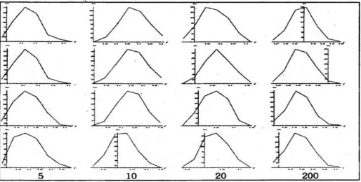
The appearance of the approximate sampling distribution for ̂
taken from the Gamma distributions is illustrated in fig.2. It is remarkable how symmetric these distributions are when the parent distributions are skewed. The sampling distribution of
̂ depends on sample size n. As sample size n increases it tends
towards symmetric distribution. For a very large sample size it becomes perfectly symmetric.
Fig. 2: Sampling distribution of G for Sample sizes 5, 10, 20 and 200.
Table-III: Confidence Interval of Type ̂ √ ( ̂)
G = 0.3395 G = 0.3125 G = 0.2910 G = 0.2734 n
̂ √ ( ̂) ̂ √ ( ̂) ̂ √ ( ̂) ̂ √ ( ̂)
5 476 475 479 478
10 479 480 474 474
20 479 480 478 476
200 481 483 481 480
In table-III the values of ( ̂), are given for the four
parameters. The coverage rate for the 500 confidence intervals of type ̂ √ ( ̂) are given, which indicate high rate of
coverage for true parameter values.
4. CONCLUSION
simulation is employed in this research to study the findings of Gini index in Gamma distribution for various income distribution. Consistent estimates were acquired with negligible error of ̂ which is approximately 0.0088% and
0.0054% respectively. Estimate of ̂ is found to be slightly
biased for smaller size samples but it decreases as the sample size is increased.
REFERENCES
1. Brunori, P., Ferreira, F. H., & Peragine, V. (2013). Inequality of opportunity, income inequality, and economic mobility: Some international comparisons. In Getting development right (pp. 85-115). Palgrave Macmillan, New York.
2.Chakraborti, A., & Patriarca, M. (2008). Gamma-distribution and wealth inequality. Pramana, 71(2), 233-243.
3. Dodge, Y. (Ed.). (2012). Statistical data analysis based on the L1-norm and related methods. Birkhäuser.
4. Johnson, N. L., Kotz, S., & Balakrishnan, N. (1995). Continuous Univariate Distributions, Vol 2, 2nd Ed. Wiley Series in Probability and Statistics.
5. Khor, N., & Pencavel, J. (2008). Measuring income mobility, income inequality, and social welfare for households of the People's republic of China.
6. Kovacevic, M. (2010). Measurement of inequality in Human Development–A review. Measurement, 35.
7. Macheras, A. (2016). Measuring Income Inequality and Economic Mobility. Econ Focus, (1Q), 32-35.
8. McDonald, J. B., & Jensen, B. C. (1979). An analysis of some properties of alternative measures of income inequality based on the gamma distribution function. Journal of the American Statistical Association, 74(368), 856-860.
9. Mirzaei, S., Mohtashami Borzadaran, G. R., & Amini, M. (2017). A comparative study of the Gini coefficient estimators based on the linearization and U-statistics Methods. Revista Colombiana de Estadística, 40(2), 205-221.
12. Singh, K., &Xie, M. (2008). Bootstrap: a statistical method. Unpublished manuscript, Rutgers University, USA. Retrieved from http://www. stat. rutgers. edu/home/mxie/RCPapers/bootstrap. pdf.
13. Weymark, J. A. (2003). Generalized Gini indices of equality of opportunity. The Journal of Economic Inequality, 1(1), 5-24.