Population Genetic Structure in the Pitcher Plant Flesh Fly Fletcherimyia fletcheri

(1)

Western University Western University

Scholarship@Western

Electronic Thesis and Dissertation Repository

4-22-2014 12:00 AM

Population Genetic Structure in the Pitcher Plant Flesh Fly

Fletcherimyia fletcheri

John R. O'Leary

The University of Western Ontario

Supervisor

Dr. Nusha Keyghobadi

The University of Western Ontario

Graduate Program in Biology

A thesis submitted in partial fulfillment of the requirements for the degree in Master of Science © John R. O'Leary 2014

Follow this and additional works at: https://ir.lib.uwo.ca/etd

Part of the Biology Commons, Evolution Commons, Genetics Commons, and the Population Biology

Commons

Recommended Citation Recommended Citation

O'Leary, John R., "Population Genetic Structure in the Pitcher Plant Flesh Fly Fletcherimyia fletcheri" (2014). Electronic Thesis and Dissertation Repository. 2017.

https://ir.lib.uwo.ca/etd/2017

This Dissertation/Thesis is brought to you for free and open access by Scholarship@Western. It has been accepted for inclusion in Electronic Thesis and Dissertation Repository by an authorized administrator of

(2)

Population Genetic Structure In The Pitcher Plant Flesh Fly Fletcherimyia fletcheri

Thesis Format: Monograph

by

John Robert O’Leary

Graduate Program in Biology

A thesis submitted in partial fulfillment of the requirements for the degree of

Master of Science

The School of Graduate and Postdoctoral Studies The University of Western Ontario

London, Ontario, Canada

(3)

Abstract

The study of population genetic structure in the pitcher plant flesh fly, Fletcherimyia fletcheri, is an important step in bettering our understanding of dispersal abilities, gene flow, and behavior in the species. In this paper, an extended sampling of populations across Algonquin Provincial Park was performed to elucidate an effective scale of genetic differentiation in F. fletcheri. Genetic differentiation between sites was compared to interceding landscape composition, and digital dispersal models were developed, testing the hypothesis that F. fletcheri uses aquatic tributaries for dispersal between peatlands. Data were collected on 613 specimens from 15 populations, and population

differentiation was analyzed using 10 microsatellite loci. Results indicated a pattern of isolation by distance in F. fletcheri with the exception of select, isolated sites. Analysis of models based on landscape composition showed no clear favoring of aquatic tributaries for dispersal.

Keywords

(4)

Co-Authorship Statement

(5)

Acknowledgements

Writing a list of people who have helped me over these last two (and a bit) years and that are deserving of my gratitude may be an impossible task; in its entirety it would make for a list as long as this thesis. The student body and faculty at Western have been

welcoming, kind-hearted, and utterly wonderful for the duration of my time here.

My supervisor, Dr. Nusha Keyghobadi, has been nothing short of amazing since the first day I arrived for my interview, I cannot thank her enough for what she has helped me to do and become in the last two years. There were components of this thesis that did not come easily to me, and she was always willing to sit down and better my understanding. In short, I know of no better professor at the university, and there are some great ones.

Other professors that helped me through my time at Western include, but are not limited to, Dr. Graeme Taylor, Dr. Ben Rubin, and Dr. Andre Lachance, Dr. Brent Sinclair, and Dr. Zoe Lindo.

My lab mates have been continually ready and willing to lend a hand whenever

roadblocks were hit in my work, as well as being unendingly kindhearted people outside of academia. I truly look forward to watching their many successes to come in the future as they move further and higher in their fields, and apologize for making any of them sit though the lunches that I brought in for lunch club, I may become a master of science, but I will never be a chef. I would like to thank Dr. Lindsay Crawford, Jenna Siu, Dr.

Gordana Rasic, Katie Millette, Dr. Daria Koscinski, Kristina Zilic, Elliot Winkler and my lab assistants Sarah Kruis and Simrat Gill.

To my wonderful family, my dad Jim O’Leary, my mom Cynthia Binnington and my sister Moira O’Leary, without all of you I would never have made it this far. Finally I would like to thank Michelle Irvine for all of her support throughout my masters and before.

To all of my friends, family, and anyone taking the time to read this, I thank you.

This work was supported by NSERC, Canada Research Chairs and Western University.

(6)

List of Tables

TABLE 1: LOCATIONS, NAMES AND ABBREVIATED (CODE) NAMES FOR PEATLANDS SAMPLED FOR F. FLETCHERI IN ALGONQUIN PARK... 16 TABLE 2: METRICS OF GENETIC DIVERSITY FOR F. FLETCHERI IN 15 SAMPLED PEATLANDS.. ... 30 TABLE 3: MATRIX OF PAIRWISE FST VALUES FOR POPULATIONS OF F. FLETCHERI FROM DIFFERENT

PEATLANDS ACROSS ALGONQUIN PROVINCIAL PARK... 32 TABLE 4: AMOVA TABLE FOR 15 F. FLETCHERI POPULATIONS ACROSS ALGONQUIN PROVINCIAL

PARK... 33 TABLE 5: CORRELOGRAM VALUES FOR TRANSFORMED PAIRWISE FST OVER 8 DISTANCE CLASSES FOR 15 F. FLETCHERI POPULATIONS ACROSS ALGONQUIN PARK... 39 TABLE 6: CORRELOGRAM VALUES FOR TRANSFORMED PAIRWISE FST OVER 7 DISTANCE CLASSES FOR POPULATIONS OF F. FLETCHERI IN ALGONQUIN PROVINCIAL PARK... 40 TABLE 7: MATRIX OF PAIRWISE “RESISTANCE COST” LEAST COST PATH VALUES... 44 TABLE 8: CORRELOGRAM VALUES FOR TRANSFORMED PAIRWISE FST FOR 13 F. FLETCHERI

POPULATIONS... 47 TABLE 9: CORRELOGRAM VALUES FOR TRANSFORMED PAIRWISE FST FOR 10 F. FLETCHERI

(9)

List of Figures

FIGURE 1: HABITAT OF F. FLETCHERI AT VARIOUS SPATIAL SCALES...9 FIGURE 2: MAP OF ALGONQUIN PROVINCIAL PARK (ONTARIO, CANADA) SHOWING ALL FIFTEEN

SAMPLED PEATLAND SITES... 23 FIGURE 3: LEAST-‐COST PATHS BETWEEN CARACAJOU PEATLAND AND EACH OF THE TWELVE OTHER

SAMPLED PEATLANDS IN ALGONQUIN PARK (EXAMPLE OF LEAST COST PATHS)... 27 FIGURE 4: PRINCIPAL COORDINATES ANALYSIS OF GENETIC DIFFERENTIATION FOR ALL 15 SAMPLED POPULATIONS... 35 FIGURE 5: SCATTER PLOT OF TRANSFORMED PAIRWISE FIXATION INDICES (FST/(1-‐FST)) RELATIVE

TO GEOGRAPHIC DISTANCE FOR ALL 15 SAMPLED PEATLAND SITES... 37 FIGURE 6: SCATTER PLOT OF TRANSFORMED PAIRWISE FIXATION INDICES (FST/(1-‐FST)) RELATIVE

TO GEOGRAPHIC DISTANCE FOR 12 SAMPLED PEATLAND SITES AFTER REMOVAL OF OUTLIER SITES FOUND IN PCOA... 38 FIGURE 7: MANTEL CORRELOGRAM OF PEARSON-‐PRODUCT MOMENT CORRELATION (R) RELATIVE

TO GEOGRAPHIC DIASTNCE FOR ALL 15 SAMPLED SITES. ... 41 FIGURE 8: MANTEL CORRELOGRAM OF PEARSON PRODUCT MOMENT CORRELATION (R) RELATIVE

TO GEOGRAHPIC DISTANCE, PCOA OUTLIERS REMOVED... 42 FIGURE 9: SCATTER PLOT OF TRANSFORMED PAIRWISE FIXATION INDICES (FST/(1-‐FST)) RELATIVE

TO RESISTANCE COST FOR 13 SAMPLED PEATLAND SITES... 45 FIGURE 10: SCATTER PLOT OF TRANSFORMED PAIRWISE FIXATION INDICES (FST/(1-‐FST))

RELATIVE TO RESISTANCE COST FOR 10 SAMPLED PEATLAND SITES POST PCOA... 46 FIGURE 11: PARTIAL MANTEL CORRELOGRAM FOR ALL SITES, COMPARING TRANSFORMED FST VS.

RESISTANCE COST WITH EUCLIDEAN DIST. AS EXPLANATORY VARIABLE... 49 FIGURE 12: PARTIAL MANTEL CORRELOGRAM FOR ALL SITES COPARING TRANSFORMED FST VS.

RESISTANCE COST AFTER REMOVAL OF OUTLIER SITES WITH EUCLIDEAN DIST. AS

EXPLANATORY VARIABLE... 50 FIGURE 13: SECTION OF RADIO OBSERVATORY (RDO) PEATLAND TAKEN IN ALGONQUIN

(10)

List of Appendices

APPENDIX 1: MODEL DEVELOPED IN ARCGIS TO PRODUCE INDIVIDUAL LEAST COST PATHWAYS FOR

F. FLETCHERI DISPERSAL... 67

APPENDIX 2: P-‐VALUES FOR TESTS OF HARDY WEINBERG EQUILIBRIUM... 68

(11)

List of Abbreviations

IBD Isolation by distance

IBB Isolation by barrier IBR Isolation by resistance

F. fletcheri Fletcherimyia fletcheri

UTM Universal transverse Mercator

S. purpurea Sarracenia purpurea

GPS Geographic positioning system

GIS Geographic information system

n Sample size

AR Allelic richness

HE Expected heterozygosity

NA Allelic diversity

cfr Cauliflower road peatland

ink Ink lake peatland

maj Major lake road peatland

mcc McIntyre’s clearing trail peatland

rdg Rod and Gun peatland

rdo Algonquin radio observatory peatland

jwl Jewel lake peatland

dmr David Mumbayaka river peatland

min Minor lake peatland (Bab lake)

whl Wolf Howl peatland

caj Caracajou peatland

brl Brent road into Cedar lake peatland

kwl Karl Wilson peatland

hgn Hogan lake peatland

prx Proulx lake peatland

PCR Polymerase chain reaction

TD Touchdown

HWE Hardy Weinberg equilibrium

LD Linkage Disequilibrium

AMOVA Analysis of molecular variance

FST Fixation index

PCoA Principal coordinates analysis

MNR Ministry of Natural Resources

GME Geospatial modeling environment

LCP Least cost pathway

DEM Slope digital elevation model

(12)

1

Introduction

1.1 Connectivity, gene flow and genetic structure

Species typically occur in non-uniform distributions across their range, displaying spatially heterogeneous patterns of abundance at various spatial scales (Forman 1995b; Anderson et al. 2010). Spatial heterogeneity in abundance can occur naturally in an environment due to preexisting biotic or abiotic barriers to migration, settlement or survival. High levels of heterogeneity can also be brought about or increased in a

landscape through anthropogenic alteration or fragmentation of previously continuous or connected habitat (Fischer and Lindenmayer 2007). Therefore, for many species, patterns of spatial variation in distribution and abundance occur within the context of a patchwork of suitable habitat separated by a matrix of less optimal or unsuitable land cover types (Forman 1995).

The amount and spatial configuration of habitat in a landscape, as well as characteristics of the intervening landscape matrix, determine the degree of isolation among populations and subpopulations of a species (Taylor et al. 1993). Landscape configuration and

(13)

Groups of populations can be classified into different models of spatial structure based on the degree of connectivity among the populations: (1) patchy populations, (2) isolated populations (sometimes called “island populations”), and (3) metapopulations (Templeton et al. 1990, Mayer et al. 2009). Patchy populations are characterized by high connectivity, or near panmixia among populations, and have the highest levels of movement among populations (Templeton et al. 1990). In isolated populations, populations are completely separate, with virtually no connectivity or movement among them (Frankham et al. 2002). A metapopulation consists of multiple spatially separate sub-populations connected by the dispersal of individuals between them (Hanski 1991; Forman 1995). Metapopulations show traits from both patchy and isolated population structures, they have varying degrees of connectivity between pairs of populations and, consequently, the genetic structure of each population patch is a byproduct of the genetic structure of its

neighboring populations, landscape connectivity, and surrounding land cover composition (Shirk et al. 2010).

(14)

1.2 Landscape Genetics

The field of landscape genetics was developed through the synthesis of two traditional fields: landscape ecology and population genetics (Manel et al. 2003). The field began to develop in the early 1990’s with the advent of high throughput genetic fingerprinting using highly variable markers (microsatellites) and increases in processing power and the subsequent improved ability to efficiently analyze geospatial data (Holderegger and Wagner 2008). Landscape genetics is focused on understanding how landscape structure shapes population genetic structure through the effects of underlying processes,

particularly gene flow and genetic drift (Storfer et al. 2007; Manel et al. 2003).

A common goal in landscape genetics research is to quantify connectivity among

populations using genetic data, and relate observed patterns of connectivity to landscape structure (Holderegger and Wagner 2008). In this way, inferences about the effects of landscape attributes on gene flow can be made (Holderegger and Wagner 2008; Wu 2004).

The use of population genetic data to infer rates of dispersal and gene flow among populations provides an important approach to developing our understanding of

connectivity among natural populations while avoiding some of the difficulties associated with direct field observation of movement (Hagler and Jackson 2001; Fischer and

Lindenmayer 2007). In mark recapture studies on smaller insects for example, the small physical size of specimens makes the placement as well as the identification of marks difficult (Mayer et al. 2009; Krawchuk and Taylor 2003). Marks could also have significant effects on flight stability, sensory efficiency, and mating success, resulting in decreased fitness for sampled specimens (Hagler and Jackson 2001). Furthermore, direct observations of movement do not necessarily immediately equate to genetic connectivity (Slatkin 1987). Normally in mark recapture studies, tagged specimens recorded in a separate population from their release are taken as a sign of successful dispersal to a new region, although such movement does not lead to genetic connectivity if the migrant does not successfully reproduce in the new population (Slatkin 1987; Manel et al. 2003).

(15)

increase in genetic drift between populations (Fischer and Lindenmayer 2007). Thus, the degree of genetic divergence between the populations can be used as an indicator of connectivity between them and, given the composition of the intervening landscape, can also be used to infer the effects of differing types of land cover on dispersal (Manel et al. 2003; Mayer et al. 2009).

Three main models are used to describe the effects of intervening landscape as an obstacle to gene flow: isolation by distance (IBD), isolation by barrier (IBB), and isolation be resistance (IBR) (Wright 1943; McRae 2006; Meirmans 2012).

Isolation by distance:

IBD is the result of the inherently limited range of dispersal of any given species,

resulting in an observable trend where individuals or populations that are geographically proximate tend to also be genetically more similar than specimens that are further apart (Wright 1943). IBD is based on spatial relationships, and therefore can be analyzed independently of landscape features that may inhibit dispersal and, consequently, is usually considered a null hypothesis in landscape genetics (Meirmans 2012; Rasic 2011).

Isolation by barrier:

IBB appears when there is a clearly delineated structure or landscape feature that limits movement between regions (Schwartz et al. 2002; Cushman and McKelvey 2006). These are often individual structures such as rivers or fences, and result in a clear decrease or cessation of movement between regions on either side of the barrier resulting in a decrease or cessation of gene flow across the barrier, however gene flow in sub

populations that are on the same side of the barrier remain unaffected (Forbes and Hogg 1999; Cushman and McKelvey 2006).

Isolation by resistance:

(16)

will depend on the connectivity among sites and the composition and configuration of intervening landscapes (McRae 2006). IBR models are based on total accumulated

resistance values, unlike IBD, which relates cost only to distance traveled. Resistance cost is based on the amount and quality of traversable landscape between sites, and takes into account distance traveled as well as dispersal resistance due to interceding landscape (McRae and Beier 2007; Graves 2012).

IBB and IBR are both a result of geographic processes, either biotic or abiotic, which can cause genetic isolation in populations. All three processes (IBD, IBR, IBB) often occur simultaneously to some extent across the range of a species, and the ability to isolate and interpret the scale of each process as it contributes to population structure is one of the main goals of landscape genetics (McGarigal and Cushman 2002; Fahrig 2003; Rasic 2011).

The understanding that landscape genetic analyses can provide about the microevolutionary processes that define genetic structure across space is highly dependent on the scale at which sampling takes place (Anderson et al. 2010). The distances among sampled populations defines the sampling grain (Wu 2004; Fortin and Dale 2005). Selecting the correct grain is important in landscape genetics studies. Species that are poor dispersers will often show increased levels of genetic isolation and greater IBD over smaller geographic ranges, thus requiring that sampling and analysis of population genetic structure be performed on a fine scale in order to detect variation among populations and individuals (Rasic and Keyghobadi 2012b; Anderson et al. 2010). Inversely, when species show a strong dispersal ability, sampling at a small scale may result in panmixia in the observed genetic structure of populations, and researchers may lose the ability to detect gene flow, broad scale barriers, or the ability to properly assess the rate and scale of gene flow among populations (Cushman and Landguth 2010).

1.3 The pitcher plant microcosm

(17)

two species are the midge, Metriocnemus knabi, and the mosquito Wyeomyia smithii

(Coquillett 1892; Harvey and Miller 1996; Dahlem and Naczi 2006). Northern purple pitcher plants occur exclusively in peatlands, including sphagnum bogs, poor fens and seepage swamps, all of which are areas of low nitrogen deposition(Ne’eman et al. 2006).

The first larval instar phase of F. fletcheri develops exclusively in the enclosed stagnant water of the fluid filled pitcher leaves; therefore, larviposition will only occur where there are living S. purpurea specimens (Johannsen 1935). The larvae of F. fletcheri use a large spiracular pit to remain afloat within the fluid filled leaves, and feed on drowned prey (Johannsen 1935). F. fletcheri larvae help the plant by breaking larger trapped prey into smaller, more easily dissolved and digested pieces (Johannsen 1935). The first instar larvae are actively territorial upon deposition into the leaf, and show cannibalistic tendencies towards other larvae, often killing any other larvae in the same leaf within 24 hours of deposition. The larger and more developed of the two larvae will usually win out (Rango 1999). Adult F. fletcheri are also dependent upon the flowers of the pitcher plant for roosting and possibly as a site for reproduction (Krawchuk and Taylor 1999). Once the larvae have approached pupation, they eat their way out of the bottom of their individual leaf, pupate, and overwinter in the peat moss at the base of their host pitcher plant (Krawchuk and Taylor 1999).

In the northern portion of its range, F. fletcheri is univoltine due to harsh winter conditions. This means that they only have one generation per year, with one active mating season and an extended dormant overwinter phase (Rango 1999; Krawchuk and Taylor 2003).

Pitcher plants and their inquiline inhabitants have been important in a variety of ecological and evolutionary studies. As with other microcosms, which include certain species of insect larvae in bromeliads, invertebrate colonies in pan shells,

(18)

pitcher plant microcosm and its members have been the focus of papers on life history evolution, inter-specific competition for shared resources, and species succession

(Bradshaw and Holzapfel 1990; Fish and Hall 1978; Hardwick and Giberson 1996). The prior use of the pitcher plant larval community to look at questions involving community ecology, ecosystem ecology, and life history evolution means that our understanding of the early life stages of the flesh fly as well as the other members of the inquiline

community is strong. However, these studies have provided relatively little information on dispersal and other life history traits after the inquiline larvae pupate and reach their adult form.

A poor understanding of adult dispersal in an ecological model system is not ideal. One of the key benefits of studying enclosed inquiline communities and other microcosms is their easily manageable size, and the ability to isolate and analyze the effects of

alterations to system parameters on species’ traits, abundance and distribution (Srivastava et al. 2004). Examples of this can be seen in studies looking at the effects of nutrient availability, species diversity, and inter-specific competition on inquiline populations undergoing different treatments in S. purpurea (Fish and Hall 1974; Hoekman 2011). A better understanding of adult dispersal and spatial population genetic structure in pitcher plant inquilines will contribute to more complete interpretation of the results of such experimental manipulations.

Recently, pitcher plant inquilines have been used to study the effects of habitat spatial structure on dispersal and gene flow due to the ability to define discrete patches of habitat for these species at multiple nested spatial scales (Figure 1) (Millette 2012; Rasic and Keyghobadi 2012b; Zilic 2013).

(19)

supports a population structure where the effects of similar landscape distances decrease in species that are stronger dispersers, such as Flectherimyia fletcheri (Rasic and

(20)

(21)

1.4 Scale of dispersal and gene flow in

F. fletcheri

Determination of appropriate sampling scale, or distance between sites, also known as the sampling “grain”, is important in landscape genetics. An improper sampling grain can have a significant impact on the conclusions drawn about effects of landscape structure on genetic differentiation (Balkenhol et al. 2009). If sampling grain is set too low, variation among sites may not be observed at all, and significant genetic differentiation may be missed in an analysis (Shirk et al. 2010). However, if the scale of sampling is too large, relevant landscape information may be overlooked, and the effect of intervening landscape on genetic differentiation of populations will be obscured (Wu 2004; Fortin and Dale 2005).

The first objective of this research was to determine the grain at which sampling of F. fletcheri would reveal significant genetic differentiation among populations in different peatlands, and allow for the study of effects of landscape on population genetic structure. Determining an effective sampling scale for F. fletcheri as well as landscape effects on connectivity is important as F. fletcheri is a key member of a heavily studied model system in ecology, yet we still know very little about its adult dispersal ability and population structure (Dahlem and Naczi 2006; Rasic and Keyghobadi 2009; Rasic and Keyghobadi 2012a). Previous studies using direct observation or mark recapture to infer dispersal rates in F. fletcheri have been unable to determine an effective sampling grain for the species, and research that did look at genetic structure recommended increases in the geographic scale of sampling in order to more effectively infer patterns of

differentiation among populations (Rasic and Keyghobadi 2012a; Krawchuk and Taylor 2003).

Observational studies looking at dispersal in adult F. fletcheri have not been able to estimate long-range dispersal (i.e. between peatlands). Previous mark recapture

(22)

following adults beyond the borders of a peatland nearly impossible (Krawchuk and Taylor 1999). Genetic analyses of F. fletcheri populations to infer dispersal and gene flow found significant IBD between two systems that were roughly 25 km apart, but not at smaller spatial scales; among peatlands within-systems, or within-peatlands (Rasic and Keyghobadi 2012a). IBD was detected only at the largest spatial scale included in the previous study indicating that an expansion of geographic scale of sampling was needed in order to fully describe patterns of genetic differentiation among F. fletcheri populations in different peatlands (Rasic and Keyghobadi 2012a).

Previous study of population genetic structure in F. fletcheri indicated that an ideal sampling design for this study should have greater distances between sampled populations (i.e. peatlands) than those used in past observational studies. A sampling grain was selected that fell just below the largest scale of the previous study on F. fletcheri population genetic structure (20 km between two bog systems), with the aim of sampling at least 10 separate populations at that scale (Rasic and Keyghobadi 2012a). Population-based sampling was used as opposed to individual-based sampling since a population-based approach is often applied when there are clearly defined habitat patches in the study landscape, and the study is taking place on a large geographic scale

(Anderson et al. 2010).

1.5 Effect of landscape on dispersal in

F. fletcheri

The second research objective was to examine the effect of landscape structure on F. fletcheri gene flow using an isolation by resistance (IBR) framework. Specifically, the hypothesis that gene flow in F. fletcheri occurs along wetland and riparian areas, where stepping stone habitat of S. purpurea plants can potentially occur, was tested.

(23)

Also, S. purpurea is very effective in the development of successful novel populations from a few founder individuals (Schwaegerle and Schaal 1979; Parisod et al. 2005). While S. purpurea is commonly observed as large colonies inhabiting discrete peatlands, it can also occur as smaller, “satellite” populations in other areas such as along riverbanks and lake edges. Small satellite populations of S. purpurea are unlikely to support self-reliant populations of F. fletcheri, but could act as layover points for F. fletcheri

undergoing extensive dispersal events. Since S. purpurea is highly dependent on waterlogged regions in order to effectively develop, the potential habitat for these “satellite” founder populations is limited to inundated areas (Gotelli and Ellison 2002). Therefore, while peatlands are geographically isolated, F. fletcheri in separatepeatland systems may be connected by small populations of S. purpurea in other wetland and riparian areas, which could act as refuges for dispersing F. fletcheri.

Two contrasting hypotheses were tested regarding two possible mechanisms of dispersal in F. fletcheri. The first is that F. fletcheri is simply a strong disperser and that individuals can travel over the forested landscape between peatland patches of habitat effectively and maintain high levels of gene flow without selecting easier routes of egress. The second hypothesis is that individuals prefer, or require, intermediate satellite populations of S. purpurea which act as stepping stones while traveling between more distant, larger pitcher plant colonies that can support populations of F. fletcheri. This would limit effective dispersal routes for F. fletcheri to corridors where S. purpurea is capable of dispersal and establishment. The most likely locations of these satellite S. purpurea

populations would be along aquatic and wetland systems connected to peatlands, due to the hydrochoric nature of the pitcher plant’s seed dispersal (i.e. dispersed by aquatic channels) (Ellison and Parker 2002).

1.6 Research questions and hypotheses

(24)

Question 1: At what spatial scale is gene flow between populations limited, such that significant genetic differentiation and isolation-‐by-‐distance is detected in F. fletcheri?

Hypothesis 1: At a spatial grain of 15-‐20 km, gene flow is sufficiently limited that there is significant differentiation among F. fletcheri populations in different bogs.

Prediction 1: Euclidean geographic distance and genetic differentiation between populations sampled at a grain of 15-‐20 km will be significantly positively

correlated, and most populations will be significantly differentiated from each other.

Question 2: Are there certain habitat types or barriers in the landscape that limit gene flow by the flesh fly?

Hypothesis 2: Wetland and riparian habitats, through the provision of satellite S. purpurea colonies, facilitate movement and gene flow in F. fletcheri, while upland forests are avoided and act as a barrier to gene flow.

Prediction 2: Resistance distances between sampled peatlands that are based on use of wetlands and riparian areas as movement corridors will be more strongly correlated with measures of genetic differentiation between F. fletcheri populations than straight-‐line geographic distance.

(25)

2

Materials and methods

2.1 Collection of specimens

Samples were collected from Algonquin Provincial Park in Ontario Canada (UTM Zone 17T/18T) during the late summer season of 2012. Potential sampling sites were first identified with the aid of the Ministry of Natural Resources cataloging project kept for Algonquin Provincial Park, which records spatially referenced species sightings across townships within the park boundaries. Searches were performed for sightings of S. purpurea, with results ranging as far back as 1901. Also, other peatland-dependent species were cross-referenced within the cataloging project to identify locations that may have been overlooked in the initial S. purpurea listing but could also contain pitcher plant communities. These peatland indicator species include bog Labrador tea, Rhododendron groenlandicum, bog cranberry, Vaccinium oxycoccos, leatherleaf Chamaedaphne

calyculata, and several genera of Sphagnum (Family: Sphagnaceae) mosses (Glaser 1992; Tiner 2002). Locations of potential sample sites were then reconsidered based on

proximity to accessible road and river routes, and interpretation of aerial imagery provided by the Ministry of Natural Resources (Ontario Ministry of Natural Resources, Forest Resource inventory for Algonquin Park, 2006). Finally, sites were scouted in spring 2012 using logging road access where possible, and canoeing and hiking trails where such access was restricted. Fifteen accessible sites were located containing S. purpurea that were large enough to potentially provide a target sample size of forty-five

F. fletcheri specimens (Table 1). A target number of forty-five specimens was set for sampling to ensure a sufficient sample size for inference of population genetic structure (Leberg 2002). Sites containing S. purpurea were visited again to collect specimens between June 24th and August 21st, 2012. Specimens were collected in their third larval instar phase. Collection of adults is more difficult due to their instinctual predator evasion mechanism in which the flies descend into the sphagnum mats and bury themselves when approached or disturbed (Krawchuk and Taylor 1999).

(26)

purpurea were inspected for the presence of F. fletcheri larvae. When a larva was found, a converted plastic Pasteur pipette with a truncated tip was used to quickly collect

specimens before they were able to swim to the base of the leaf and conceal themselves in detritus. Individuals at each peatland were removed from separate plants in an attempt to avoid sampling direct siblings (Forsyth and Robertson 1975). Sampling was also

expanded to encompass a greater search radius in larger peatlands to avoid sampling a subsection of the peatland.

Once samples had been collected, larvae were immediately placed into a separate 100% ethanol solution, and the location of each individual sample collected was recorded using a high accuracy GPS receiver accurate to 1.5 m (Trimble GeoXH geoexplorer 2005 series, Westminster CO, USA), within a minimum satellite count set to 6 to ensure 1.5 m accuracy. All samples were rinsed with 100% ethanol upon return to base camp, placed in a new 1.5 ml Eppendorf of 100% ethanol, and maintained at -20°C to minimize DNA and

tissue degradation. Geographic location data were stored in Terrasync GPS software (ver. 3.21, ®Trimble Nav. Ltd. Sunnyvale CA, 2008) until transferred to GPS Pathfinder

Office (ver. 4.10, ®Trimble Nav. Ltd. Sunnyvale CA, 2008) and finally converted to

(27)

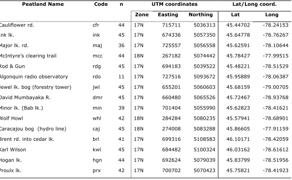
Table 1: Locations, names and abbreviated (code) names for peatlands sampled for F. fletcheri in Algonquin Park. Locations of bogs are given in UTM NAD 1983 coordinates, as well as decimal degrees of latitude and longitude, ‘n’ represents the number of larvae sampled from each peatland.

Peatland Name Code n UTM coordinates Lat/Long coord.

Zone Easting Northing Lat Long

Cauliflower rd. cfr 44 17N 715711 5036313 45.44702 -78.24153

Ink lk. ink 45 17N 674336 5057350 45.64778 -78.76267

Major lk. rd. maj 36 17N 725557 5056558 45.62591 -78.10644

McIntyre’s clearing trail mcc 44 18N 267182 5074442 45.78427 -77.99515

Rod & Gun rdg 45 17N 694183 5039522 45.48221 -78.51529

Algonquin radio observatory rdo 11 17N 727516 5093672 45.95889 -78.06387

Jewel lk. bog (forestry tower) jwl 45 17N 655201 5060603 45.68159 -79.00705

David Mumbayaka R. dmr 45 17N 660480 5065526 45.72467 -78.93768

Minor lk. (Bab lk.) min 39 17N 701404 5055990 45.62823 -78.41621

Wolf Howl whl 42 18N 284284 5080235 45.57941 -78.68901

Caracajou bog (hydro line) caj 45 18N 274008 5083288 45.86605 -77.91159

Brent rd. into cedar lk. brl 41 17N 699316 5108583 46.10171 -78.42059

Karl Wilson kwl 45 17N 684482 5100324 46.03162 -78.61612

Hogan lk. hgn 44 17N 692624 5079039 45.83799 -78.51956

(28)

2.2 DNA extraction and microsatellite analysis

DNA was extracted from individual F. fletcheri larvae using the DNEasy Blood and Tissue Extraction Kit (®QIAGEN, Germantown, MD). Sample extraction was modified so that only 100µL of elution buffer was used, allowing for a higher concentration of DNA in the final solution. The quantity of DNA in extracted samples was determined before PCR analysis using a spectrophotometer (Shimadzu Biotech Bio-spec Mini DNA/RNA protein analyzer spectrophotometer, λ260, λ280, and λ230) (®Shimadzu Biotech, Manchester, UK). Samples were confirmed to have concentrations ranging from 85µg/mL to 223µg/mL of DNA in successfully extracted samples.

Larvae were genotyped at 11 microsatellite loci developed specifically for F. fletcheri: FF104, FF72, FF10, FF189, FF231, FF09, FF249, FF62, FF238, FF82 and FF65 (Rasic and Keyghobadi 2009). PCR amplification of the microsatellites occurred with one reaction of 6 PCR loci (FF104, FF72, FF10, FF189, FF231 and FF09), one multiplex of two loci (FF 249 and FF62), and individual amplifications of the remaining three loci (FF65, FF238 and FF82) (Rasic and Keyghobadi 2009). PCR amplifications were performed in a PTC 0200 DNA Engine Cycler (BioRad, Hercules, CA). PCR reactions occurred in a final solution of volume 20µL; each amplification contained 1x PCR Buffer

(50 mM KCl, 10 mM Tris-HCl pH 8.3 at room temperature), 3.75 mM MgCl2, 0.15

mg/ml bovine serum albumin (BSA), 0.3 mM of each dNTP, 1.5 U of AmpliTaq DNA polymerase (Applied Biosystems, Foster City, CA), and approximately 300 ng of F.

fletcheri DNA (Rasic and Keyghobadi 2009). Concentrations of F. fletcheri DNA were

(29)

PCR thermal cycling profiles followed one of four protocols as follows (Rasic and Keyghobadi 2009):

(1) FF231, FF217, FF189, FF238, FF10, FF72, FF104, FF9:

Denaturation for 180s at 96°C; 2 cycles of 30s at 96°C; 30s at 60°C; 30s at 72°C;

14 touchdown (TD) cycles of 15s at 96°C; 15s at 60°C (-0.5°C each cycle); 15s at 72°C; 17 cycles of 15 at 96°C, 15s at 53°C, 15s at 72; and final elongation at

72°C for 180s.

(2) FF065:

Denaturation for 180s at 96°C; 2 cycles of 30s at 56°C, 30s at 72°C; 12 TD cycles

of 15s at 96°C, 15s at 56°C (-0.5°C each cycle), 15s at 72°C; 20 cycles of 15s at

96°C, 15s at 50.5°C, 15s at 72°C; and a final elongation step of 180s at 72°C.

(3) FF249, FF62:

Denaturation for 180s at 96°C; 2 cycles of 30s at 96°C, 30s at 53°C, 30s at 72°C;

6 TD cycles of 15s at 96°C, 15s at 53°C (-0.5°C each cycle), 15s at 72°C; 25 cycles of 15s at 96°C, 15s at 50.5°C, 15s at 72°C, and a final elongation for 180s at 72°C.

(4) FF82:

Denaturation for 180s at 96°C, 30 cycles of 30s at 96°C, 30s at 50°C, 30s at 72°C,

and a final elongation step of 180s at 72°C.

PCR products were sent to Michael Smith Laboratories at the University of British

Columbia for fragment size analysis in an Applied Biosystems® 3730S 96 capillary DNA Analyzer, using LIZ-500 as a size standard. The multiplex PCR was diluted to 1:1 with H2O and loaded onto a single lane of the DNA analyzer. The five remaining loci were

mixed in the following proportions and loaded together in a single lane of the DNA analyzer: 5 H2O: 1.5 FF249+FF62: 1 FF65: 1 FF238: 1 FF82.

Electropherograms generated by the DNA analyzer were processed and reviewed using Genemapper software Ver. 4.0 (®Applied Biosystems 2005) to determine microsatellite

(30)

2.3 Hardy Weinberg and Linkage Disequilibrium tests

Tests for Hardy Weinberg equilibrium (HWE) and linkage disequilibrium were run in Arlequin 3.11 (Excoffier et al. 2005).

Tests for HWE were run using an allowed level of missing data of 0.05, 1000000 steps in the Markov chain, and 100000 steps of Dememorisation, using the method for HWE test for populations using multiple alleles as outlined by Guo & Thompson (1992). This test is analogous to a Fisher’s exact test, with a triangular contingency table of arbitrary size instead of a two by two contingency table (Guo and Thompson 1992). It is designed and recommended for use in populations where the number of samples in each site is low (typically, n<50), and there is no allelic masking, that is, the zygotic state of a diploid organism is fully know at each locus (Peakall and Smouse 2012; Guo and Thompson 1992).

2.4 Metrics of diversity

Metrics of within-population genetic diversity were measured using Genalex 6.5 (Peakall and Smouse 2012): expected heterozygosity (HE) averaged over loci was measured for

each peatland. Allelic diversity (NA) and mean allelic richness (AR), which is a measure

of allelic diversity corrected for sample size, was also averaged over loci (Table 2). In this case NA is defined as the number of alleles found at each loci determined by direct count

and averaged over all observed locus for each site (Slatkin 1995). AR is also a direct count

of alleles at each locus then averaged over all observed loci for a site, however it is rarified to the smallest number of alleles sampled (Leberg 2002). Allelic richness was calculated in the program allelic.richness() from the Hierfstat program library in R 2.14.1, and rarified to a sample size of 11, with an allele count of 22 (the smallest sample size collected) (Goudet 2005).

2.5 AMOVA and pairwise F

ST

(31)

of populations and among groups), along with estimation of variance components and F statistics (or fixation indices) and hypothesis tests for fixation indices using

non-parametric permutation procedures (Excoffier et al. 1992). Fixation indices are measures of genetic differentiation at the respective level of the nested hierarchy.

In this study, there were three nested levels of structure: among-peatlands, within-peatlands, and within-individuals. Also, genetic differentiation between sampled populations was analyzed using pairwise fixation indices (pairwise FST), and tested for

significance using permutation procedures. It is important to note that FST is a statistic

used when trying to determine an effective estimate of θ, or the correlation of genes

across individuals in a population as a measure of coancestry, and is not an estimate of FIS, which is a direct measure of inbreeding within populations (Clarke and Weir 1984).

Pairwise FST was used as a measure of subpopulation differentiation rather than a metric

modeled after a step-wise mutation model, such as RST. A step-wise mutation model may

be more theoretically accurate in describing the mechanism of genetic differentiation of microsatellite alleles, however studies of population structure in real populations have shown that a step-wise model rarely holds true (Excoffier et al 1992).

2.6 Principal Coordinates Analysis (PCoA)

A principal coordinates analysis, or multidimensional scaling, was performed on pairwise FST values to visualize relationships among peatland populations using Genalex 6.5.

Classical multidimensional scaling uses an input matrix of pairwise distances and develops coordinate axes in multiple dimensions, these axes minimize the distances among points, also known as minimizing strain, and attempt to explain the maximal variation in distances in the fewest axes possible(Orlóci 1978; Peakall and Smouse 2012). The model describes proportionately less and less variance with each successive axis, and if there are no distinct groups within the input matrix, in our case pairwise FST

(32)

2.7 Isolation by Distance analysis

Analysis of IBD in F. fletcheri was performed using standard Mantel tests of correlation and Mantel correlograms. A geographic distance matrix was computed using the

Euclidean (straight-line) distance (in meters) between the geometric center of each sampled peatland and the center of all 14 other sampled peatlands. To determine the geometric centers of peatlands, Ontario Ministry of Natural Resources (MNR) land cover maps of Algonquin Park were used where possible. Peatlands that fell outside of the park boundaries (Cauliflower rd. and Brent rd. into Cedar, a.k.a. cfr and brl) were measured using images taken from the Ontario MNR provincial land cover index for southern Ontario (Table 1)(Ontario Ministry of Natural Resources, Forest Resource Index, province wide, 5m2 resolution, 2005). The matrix of Euclidean distances was calculated using arcGIS 10.1 and Geospatial Modeling Environment 0.7.2.1 (GME), an external program with accessory functions for spatial analysis in arcGIS 10.1 (ArcGIS Ver. 10.1, ®ESRI, Redlands, CA; GME 0.7.2.1 Spatial ecology LLC, Queensland, AUS). The

command pointdistances was used in GME and set to measure straight-line distances from the geometric center of each peatland to the center of the other 14 sampled sites.

A second matrix of transformed pairwise fixation indices (FST) was developed using

pairwise FST values calculated in Genalex 6.1 (see section 2.5) and transformed in R

2.14.1 using the following equation (Venables et al. 2002):

The linearization transformation above is recommended by Rousset (1997) for IBD analysis in two dimensional landscapes.

(33)

Sturges’ Rule was used to determine the most effective number of break points when developing our Mantel correlograms using the function pmgram() from the Ecodist package (Goslee and Urban 2007; Mantel 1967). Sturge’s rule is as follows:

(34)

(35)

2.8 Isolation by resistance

To test the hypothesis that F. fletcheri uses riparian and wetland areas as dispersal corridors between populations, a “resistance surface” was built in ArcGIS that would reflect this hypothesis, and least cost paths (LCP) between sites were calculated. A resistance surface is a digitized matrix representing a landscape and the permeability of the landscape to animal movement (McRae 2006). The matrix is composed of a

continuous series of spatially referenced pixels, and each pixel is given a resistance value or “cost” for the organism to cross it (Koen et al. 2012). Different landcover classes are assigned different costs to traverse; the easier the landscape is to move through for a given species, the lower the associated cost for that landcover type on the resistance surface (McRae 2006; Koen et al. 2012). Cost values can be assigned from independent movement data (e.g. telemetry or mark recapture), based on expert opinion, or based on a specific hypothesis to be tested about movement through the landscape (as in this study). The total cost of moving across a series of pixels within the resistance surface represents the cost of migration for an animal as it moves across the landscape. A least cost pathway is the route between two sites over a resistance surface (in our case, two peatlands) that would have the lowest total accumulated cost (sum of resistance values for each pixel traversed) for an individual, and is a byproduct of both distance traveled and difficulty of interceding terrain (Etherington and Holland 2013).

(36)

corridors, rather than being corrupted by overshadowing of terrestrial land cover, as often occurs in raster maps developed using aerial photography containing overlapping land cover classes (Heywood et al. 2006). The merged vector layer was then converted to a raster layer using arcGIS’s vector to raster toolbox, and was given a resolution of 5m2. A raster grid represents an actual landscape artificially through an equally sized repeating tessellation (tessellations are repeated connections using a specific geometric shape; in this case, squares). This tessellated surface creates a matrix of data points, where each individual square is given a value or values that can represent a specific component of the landscape that is being isolated and analyzed (in this case, land cover type). Nearest neighbor conversion of vector to raster was used to maintain connectivity of raster polylines. In the newly created raster, two resistance values were used to create a binary pass/impasse resistance matrix. Terrestrial ecosystems, such as grasslands, upland forest, and any other landcover type that fell outside of wetland or aquatic environment were considered impassable and were graded as significantly more difficult to traverse than wetland, river, and open water. Landcover hypothesized to be non-passable was given a resistance value 50 times greater than landcover considered passable (resistance value of 50 for non-passable habitat; and 1 for passable habitat). Therefore to test the LCP

hypothesis, a binary raster surface with strong contrast between passable and impassable land was developed. This binary comparison of landcover types represents the most direct test of the hypothesis that F. fletcheri movement is limited to wetland and aquatic areas. A strong contrast in resistance of passable and impassable landcover means that least cost pathways will strongly follow riparian and wetland corridors, and only allow for very small “jumps” over non-passable landcover before resistance cost is heavily affected by non ideal landcover traverses. Biologically, this reflects a hypothesis of very strong reliance on wetland, riparian, and water covered areas for movement, and a strong tendency to avoid movement over other landcover types for F. fletcheri.

After the initial resistance surface was developed, the 13 sites that were located within the park boundaries (which had sufficient data on landscape composition within the

(37)

12 sampled peatlands (Appendix 1). Slope Digital Elevation Models (DEMs) were used to allow for inherent data on directionality in watersheds, but were normalized to 0 in keeping with the airborne nature of F. fletcheri, which, it was hypothesized, should not be affected by direction of water flow. Least cost pathways were allowed with diagonal connectivity using Manhattan distances instead of Pythagorean connections and eight neighbor joining of cells to avoid overestimations of weighted distance values due to a “staircase” effect (Heywood et al. 2006).

The significance of partial correlation between pairwise LCP distance and transformed pairwise FST, controlling for Euclidean geographic distance, was tested using a partial

Mantel test in R 2.14.1 using the package mantel.partial() from the Vegan library (Venables et al. 2002; Oksanen et al. 2010). A partial Mantel functions similarly to a standard Mantel. However, in addition to the initial two compared variables, the partial Mantel also includes a third matrix of data points. This third matrix is used as an explanatory variable (geographic distance), to better isolate the effect of a specific independent variable (land cover type) on the dependent variable (genetic variation, represented in this instance by transformed FST). A partial correlogram was developed

(38)

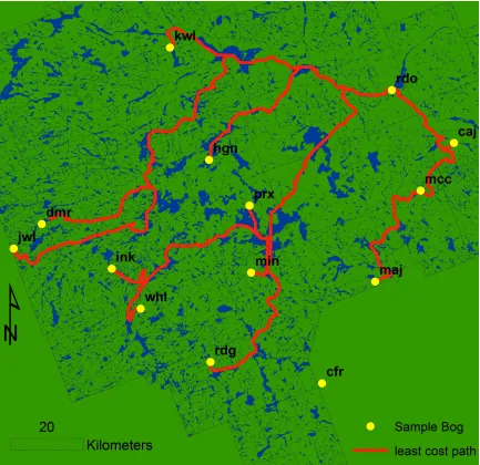
Figure 3: Least-‐cost paths between Caracajou peatland and each of the twelve other sampled peatlands in the park. Paths represent routes of least “resistance” or “cost”, assuming that the resistance provided by aquatic, riparian and wetland landcover is two percent that provided by other land cover classes. Note that site cfr is not included in the development of least cost path analyses. Cfr is one of two sites (along with brl) that fell outside of the park boundaries. As a result, landcover information was not available for cfr and its surrounding region, and a least cost path could not be developed for it.

(39)

3

Results

3.1 Microsatellite variability

DNA was extracted from 641 individual larvae, from which the alleles of selected microsatellite loci were successfully amplified for 613 specimens. Specimens that failed to amplify initially were re-run, and, if they failed a second time, were removed from further analysis. Any individual that had more than two absent loci was also removed from analysis. Out of the 613 specimens for which microsatellites successfully amplified, four individuals were missing alleles at one locus, and one individual was missing alleles at two loci.

The total number of alleles observed at each locus ranged from two to twelve within each peatland, and all eleven loci were polymorphic across all fifteen peatlands sampled. From this it was determined that there was a moderate amount of microsatellite genetic

diversity within the 15 separate sites, with mean allelic diversity (NA) ranging from 3.40

(Algonquin radio observatory, rdo) to 6.00 (Brent lake road, brl) and an expected

heterozygosity (HE) of between 0.431 (Minor Lake, min) and 0.569 (Brent Lake road, brl)

(Table 1). Allelic richness (AR) ranged from 3.20 to 4.36 (Table 2). Therefore, AR did

remove some of the variation seen in the initial measure of NA that was caused in part by

varied sample size across sites (Table 1).

(40)

(41)

Table 2: metrics of genetic diversity for F. fletcheri in 15 sampled peatlands. NA

represents mean allelic diversity averaged across 10 loci; AR represents allelic

richness, which is the mean allelic diversity over all loci adjusted for sample size; HE represents expected

heterozygosity.

Peatland NA(±SE) AR HE(±SE)

min 4.50(0.86) 3.36 0.43(0.06)

cfr 4.60(0.40) 3.36 0.46(0.06)

maj 3.90(0.55) 3.21 0.46(0.05)

ink 5.40(0.78) 3.71 0.50(0.05)

whl 4.90(0.88) 3.65 0.53(0.05)

brl 6.00(0.83) 4.36 0.56(0.06)

kwl 5.30(0.97) 3.67 0.51(0.06)

mcc 5.00(0.93) 3.76 0.54(0.06)

rdg 4.90(0.71) 3.80 0.51(0.05)

jwl 4.60(0.70) 3.51 0.51(0.05)

dmr 5.20(0.81) 3.72 0.54(0.04)

rdo 3.40(0.56) 3.20 0.48(0.07)

caj 4.50(0.65) 3.54 0.47(0.05)

hgn 5.40(0.82) 3.80 0.54(0.04)

(42)

3.2 AMOVA

Globally, three percent of microsatellite variance could be attributed to genetic

differentiation among populations in different peatlands (Table 4). Four percent could be attributed to within-population variance, and the remaining ninety three percent was attributed to within-individual variance (Table 4). Global FST was estimated at 0.027 and

significantly greater than zero (p<0.001). FST was used for further analyses as levels of

expected heterozygosity within sites was not overly inflated (>0.9) and therefore should not arbitrarily skew FST results through compression (Meirmans and Hedrick 2011).

Pairwise FST values showed significant genetic differentiation between most pairs of

sampled populations at α = 0.05 (Table 3). Notably however, several populations were not significantly differentiated from Hogan Bog (hgn), a large centrally located peatland in the park (Table 1, Table 4, Figure 2). Conversely, Algonquin radio observatory (rdo) had the highest differentiation from other populations, with its lowest pairwise FST being

(43)

Table 3: Matrix of pairwise FST values for populations of F. fletcheri from different peatlands across Algonquin Provincial

Park. * indicates FST is not significantly greater than zero; p>0.05.

min cfr maj ink whl brl kwl mcc rdg jwl dmr rdo caj hgn

cfr 0.027

maj 0.034 0.036

ink 0.053 0.029 0.024

whl 0.055 0.029 0.037 0.019

brl 0.054 0.035 0.043 0.027 0.029

kwl 0.041 0.016 0.037 0.020 0.013 0.025

mcc 0.049 0.020 0.050 0.027 0.020 0.037 0.018

rdg 0.049 0.013 0.041 0.006* 0.014 0.027 0.014 0.004*

jwl 0.030 0.009 0.019 0.010 0.002* 0.020 0.004* 0.012 0.008

dmr 0.058 0.038 0.025 0.011 0.007* 0.032 0.020 0.034 0.024 0.009

rdo 0.169 0.122 0.092 0.077 0.080 0.103 0.119 0.080 0.085 0.085 0.073

caj 0.041 0.027 0.027 0.034 0.022 0.044 0.031 0.038 0.028 0.015 0.033 0.108

hgn 0.043 0.019 0.041 0.012 0.011 0.026 0.006* 0.005* 0.001* 0.003* 0.019 0.101 0.019

(44)

Table 4: AMOVA table for 15 F. fletcheri populations across Algonquin Provincial Park based on genotypes at 10 microsatellite loci. Source indicates the nested scale that is being analyzed. df represents degrees of freedom, SS is the sum of squares, MS the mean squares, Est. Var. is the estimated variance for each calculation, and % indicates the total percentage of molecular variance that can be attributed to each scale of population organization.

Source df SS MS Est. Var. %

Among Pops 14 119.85 8.56 0.07 3%

Within-Pops 598 1598.35 2.67 0.11 4%

Within-Indiv. 613 1503.87 2.45 2.45 93%

Total 1225 3222.08 2.64 100%

(45)

3.3 Principal Coordinates Analysis

PCoA results indicated that populations in Algonquin radio observatory, Major lake, and Minor lake peatlands (rdo, maj, and min), were highly differentiated from the other sample populations, as well as from each other. The first three principal axes accounted

for 76.51% of variance seen in pairwise FST between populations, with 64.24% described

(46)

Figure 4: Principal coordinates analysis of genetic differentiation for all 15 sampled populations of F. fletcheri sampled based on pairwise genetic distance matrix (FST) between peatlands. The first two principal coordinate axes are shown. The unit of measure for each axis are not shown because PCoA uses eigenvectors and eigenvalues derived from the original dataset that do not have specific units of measure.

min

cfr

maj

ink whl brl kwl

mcc rdg

jwl dmr rdo

caj

hgn prx

Coord. 2

Coord. 1

(47)

3.4 Isolation by distance

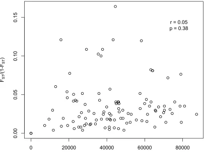
A scatter plot of transformed fixation indices (transformed FST) and geographic distance

for all sites sampled as well as a Mantel correlogram showed no clear pattern of spatial correlation, indicating a lack of IBD (Figure 5, Figure 7). The overall Mantel statistic r across all 15 sites was 0.0543, with a p-value of 0.378. This is also indicative of a lack of correlation between genetic diversity and simple Euclidean distance, and is

non-supportive of a genetic structure that is undergoing IBD given the scale sampled and molecular markers used. However, upon examination of the principal coordinates analysis for possible outliers that could be interfering with the correlation results, Algonquin radio observatory, Minor lake, and Major lake rd. (rdo, min, and maj) sites were removed from the Mantel analyses, and the overall Mantel correlation statistic increased to 0.49 (r), with a significance of 0.0006 (Figure 6).

(48)

Figure 5: Scatter plot of transformed pairwise fixation indices (FST/(1-‐FST)) relative to geographic distance for all 15 sampled peatland sites across Algonquin Provincial Park with Mantel Pearson product-‐moment correlation value (r) and corresponding p-‐value (p) included.

0 20000 40000 60000 80000

0.00

0.05

0.10

0.15

Geographic distance (m) FST

/(1

-FS

T

)

(49)

Figure 6: Scatter plot of transformed pairwise fixation indices (FST/(1-‐FST)) relative to geographic distance for 12 sampled peatland sites across Algonquin Provincial Park after removal of outlier sites identified in PCoA analysis. With Mantel Pearson product-‐moment correlation result (r) and corresponding p-‐value (p) included.

0 20000 40000 60000 80000

0.00

0.01

0.02

0.03

0.04

Geographic distance (m) FST

/(1

-FS

T

)

r = 0.49

(50)

Table 5: Correlogram values for transformed pairwise FST over 8 distance classes for 15 F.

fletcheri populations across Algonquin Park r is the value of the Mantel correlation, and (p), the associated p value (significance) for each distance class.

Distance class

(median, m) n in group r P

5008.37 2 0.71 0.26

15025.12 9 -0.12 0.74

25041.87 18 0.11 0.61

35058.62 16 -0.11 0.63

45075.37 24 0.05 0.79

55092.12 10 0.01 0.97

65108.87 14 -0.13 0.63

75125.62 10 -0.06 0.87

(51)

Table 6: Correlogram values for transformed pairwise FST over 7 distance classes for populations of F. fletcheri in Algonquin Provincial Park across 12 peatland sites after the removal of rdo, min, and maj populations.

Distance class

(median, m) n in group r p

5723.86 3 0.03 0.97

17171.57 6 0.89 0.02

28619.28 11 0.60 0.04

40067.00 16 0.00 0.99

51514.71 10 0.21 0.51

62962.42 10 -0.58 0.05

(52)

Figure 7: Mantel Correlogram of Pearson-‐Product Moment correlation (r) over 10 km distance classes for all 15 sampled sites. Sites that fell within each 10 km distance class were separated and individual Mantel tests were run using transformed FST versus geographic distance. No significant trend in genetic correlation relative to distance that would indicate IBD is shown. Error bars indicate 95% significance level. Distance class 1 (5 km median) shows no error bars due to the use of only 2 sites with 1 corresponding distance between the (therefore no variance in correlation can be calculated for that class).

1 2 3 4 5 6 7 8

-0 .4 -0 .2 0.0 0.2 0.4 0.6

Distance classes (1=10km)

(53)

Figure 8: Mantel correlogram of Pearson Product Moment Correlation (r) versus geographic distance. Distance classes of 15 km were used for F. fletcheri populations across Algonquin Park after the removal of PCoA outlier sample sites. Distance classes have been increased to 15 km in accordance with Sturge’s Rule for implementing break points.

1 2 3 4 5 6 7

-1

.0

-0

.5

0.0

0.5

1.0

Distance class (1=15km)

Pe

aso

n

Pro

du

ct

-Mo

me

nt

C

orre

la

tio

n

(54)

3.5 Isolation by Resistance (IBR)

No correlation was found between LCP distance and transformed FST after controlling for

Euclidean distance for all 15 sampled populations (r= -0.28, p=0.99). After removing Algonquin radio observatory, Minor lake, and Major lake rd. (rdo, min and maj), there

was still no significant correlation between LCP distance and transformed FST, controlling

for Euclidean distance (r= - 0.18, p= 0.91). These general results did not change when both LCP and Euclidean distances were log transformed, or when Nei’s standard genetic

distances were used in place of transformed FST (results not shown). Correlograms also

showed no pattern of spatial correlation in transformed FST values based on LCP

(55)

Table 7: Matrix of pairwise “resistance cost” least cost path values between peatlands from which F. fletcheri were sampled. kwl jwl dmr ink hgn prx min whl rdg maj mcc caj rdo

kwl 0

jwl 101954 0

dmr 57198 124812 0

ink 77463 43249 100128 0

hgn 47668 68796 53907 44116 0

prx 90829 71795 60741 44613 27005 0

min 98316 83735 62542 56557 43303 18085 0

whl 96315 62651 65399 17882 62687 45216 57136 0

rdg 121186 90806 92022 43224 87566 47884 37242 32639 0

maj 116398 112095 80628 84918 86678 46383 46168 85616 77659 0

mcc 90449 131795 35806 104617 87151 66196 67987 105422 97472 31847 0

caj 81104 148417 130047 123448 77818 84642 86442 123886 115923 52823 18756 0

(56)

Figure 9: Scatter plot of transformed pairwise fixation indices (FST/(1-‐FST)) relative

(57)

Figure 10: Scatter plot of transformed pairwise fixation indices (FST/(1-‐FST))

(58)

Table 8: Correlogram values for transformed pairwise FST for 13 F. fletcheri populations

over 7 distance classes, based on LCP resistance costs between peatland sites, based on total calculated LCP cost resistance.

Range median (resistance cost)

n in

group r p

18648 2 -0.23 0.66

37296 8 -0.45 0.26

55944 13 0.22 0.37

74591 15 -0.33 0.29

93239 19 0.15 0.53

111887 10 0.06 0.90

(59)

Table 9: Correlogram values for transformed pairwise FST for 10 F. fletcheri populations

(rdo, min & maj excluded) over 6 distance classes, based on total calculated LCP cost resistance.

Range median

(resistance cost) group n in r p

21756 2 -1.62 0.02

43512 5 -0.10 0.76

65268 10 0.14 0.63

87023 8 -0.10 0.76

108779 12 0.46 0.09

(60)

Figure 11: Partial Mantel Correlogram for all sites, comparing transformed fixation indices (Transformed FST) versus cost resistance, while controlling for Euclidean

distance by using geographic distance as an explanatory variable.

1 2 3 4 5 6 7

-0

.8

-0

.6

-0

.4

-0

.2

0.0

0.2

0.4

Distance class (1=18000 Resistance Units)

Pe

arso

n

Pro

du

ct

-Mo

me

nt

C

orre

la

tio

n

Population Genetic Structure in the Pitcher Plant Flesh Fly Fletcherimyia fletcheri

Scholarship@Western

Scholarship@Western

Population Genetic Structure in the Pitcher Plant Flesh Fly

Population Genetic Structure in the Pitcher Plant Flesh Fly

Fletcherimyia fletcheri

Fletcherimyia fletcheri

Abstract

Keywords

Co-Authorship Statement

Acknowledgements

Table of Contents

List of Tables

List of Figures

List of Appendices

List of Abbreviations

1

Introduction

1.1 Connectivity, gene flow and genetic structure

1.2 Landscape Genetics

1.3 The pitcher plant microcosm

1.4 Scale of dispersal and gene flow in

F. fletcheri

1.5 Effect of landscape on dispersal in

F. fletcheri

1.6 Research questions and hypotheses

2

Materials and methods

2.1 Collection of specimens

2.2 DNA extraction and microsatellite analysis

2.3 Hardy Weinberg and Linkage Disequilibrium tests

2.4 Metrics of diversity

2.5 AMOVA and pairwise F

2.6 Principal Coordinates Analysis (PCoA)

2.7 Isolation by Distance analysis

2.8 Isolation by resistance

3

Results

3.1 Microsatellite variability

3.2 AMOVA

3.3 Principal Coordinates Analysis

3.4 Isolation by distance

3.5 Isolation by Resistance (IBR)