DEBoost: A Python Library for Weighted Distance Ensembling in Machine Learning

(1)

DEBoost: A Python Library for Weighted Distance

Ensembling in Machine Learning

Department of Statistics and Applied Probability National University of Singapore

Blk S16, Level 7, 6 Science Drive 2, Singapore 117546

Editor:N.A. (Preprint)

Abstract

In this paper, we introduce deboost, a Python library devoted to weighted distance en-sembling of predictions for regression and classification tasks. Its backbone resides on the scikit-learn library for default models and data preprocessing functions. It of-fers flexible choices of models for the ensemble as long as they contain the predict

method, like the models available from scikit-learn. deboost is released under the MIT open-source license and can be downloaded from the Python Package Index (PyPI) at

https://pypi.org/project/deboost. The source scripts are also available on a GitHub repository athttps://github.com/weihao94/DEBoost.

Keywords: ensemble learning, machine learning, Python, spatial distance, statistical distance, weighted ensemble

1. Introduction

Ensemble learning usually refers to methods that involve the combination of several models to perform a prediction, either in classification or regression problems. In many cases, ensembles perform better than a single model. They also reduce the likelihood of the selection of a model with poor performance [ Dietterich (2000)]. In recent years, most of the research on ensemble learning was done on classification problems which unfortunately are not entirely applicable to regression problems [ Mendes-Moreira et al. (2012)].

Some commonly used ensemble algorithms are bagging (bootstrap aggregating), boosting (an ensemble of models by resampling the data, which are then combined by majority voting) and stacking (a combination of models via a meta-classifier or meta-regressor). There have been recent research done on ensemble of model predictions via spatial and statistical techniques such as Bayesian model averaging, geostatistical output perturbation and spatial Bayesian model averaging (a combination of the two) [ Berrocal et al. (2007)]. Distance weighting measures on predictions were also researched upon, for example the usage of inverse distance weighting to improve predictions in one-dimensional time series analysis with singular spectrum analysis [ Awichi and M¨uller (2013)]. In our deboost

Python library, we utilize existing distance metrics to obtain weighted ensembles of model predictions, for the classification and regression tasks. The library also utilizes well-known regression and classification models as default models. Users are able to make their own configuration to the set of default models used in the ensemble.

(2)

In the subsequent sections, we first introduce the distance metrics available in the initial release of the library, describe the computations of the weighted ensemble, introduce the library and finally present experimental results on some publicly available datasets.

2. Distance Metrics

In the version of the library’s initial release, the available distance metrics for computation of the ensembles of predictions in regression, and prediction class probabilities in classifica-tion are: Bray-Curtis, Canberra, Chebyshev, City Block (Manhattan), correlaclassifica-tion, Cosine, Euclidean, Hamming and Jaccard-Needham dissimilarity. Other non-distance metrics made available are the mean, median and Bhattacharyya distance. We now formally define each of the available spatial and statistical distance metrics.

Supoose for a regression context, that we havemregression modelsm1, . . . , mm ∈M, where

the models’ predictions aren×1 matricesY1, . . . , Ym respectively. Here, thekth observation

of Yi is denoted as Yik, where k ∈ {1, . . . , n}. Define d(Yi, Yj) as the number of elements

in Yi and Yj that differ at the same index. Also define A11, A01, A10, A00 respectively as

the total number of attributes where Yi and Yj both contain the value 1, the attribute

of Yi is 0 and the attribute of Yj is 1, the attribute of Yi is 1 and the attribute of Yj is

0, and where Yi and Yj both have a value of 0. Then between any Yi and Yj for i 6= j,

the Bray-Curtis distance, Canberra distance, Chebyshev distance, City Block (Manhattan) distance, correlation distance, Cosine distance, Euclidean distance, Hamming distance and Jaccard-Needham dissimilarity are respectively:

dBC =

Pn

k=1|Yik−Yjk|

Pn

k=1|Yik+Yjk|

, (1)

dCB = n

X

k=1

|Yik−Yjk|

|Yik|+|Yjk|

, (2)

dCH = max

k |Yik−Yjk|, (3)

dM AN = n

X

k=1

|Yik−Yjk|, (4)

dCORR = 1−

hYi−Pnk=1Yik/n, Yj−Pnk=1Yjk/ni

kYi−

Pn

k=1Yik/nk2kYj−

Pn

k=1Yjk/nk2

, (5)

dCOS= 1−

hYi, Yji

kYik2kYjk2

, (6)

dEU =kYi−Yjk2, (7)

dHAM =

d(Yi, Yj)

(3)

dJ AC=

A01+A10

A01+A10+A11

. (9)

Next, we have the Bhattacharyya distance betweenYi and Yj defined as:

dBHC=−ln

2n

X

k=1

p

p(Y_k)q(Y_k) (10)

where 2nis the total number of observations in Yi and Yk combined, and p(·), q(·) are the

histogram probabilities of the distribution of Yi and Yj respectively, and p(Yk), q(Yk) are

the histogram probabilities of the kth observation in the sequence of values in ascending order formed by concatenating the prediction arrays of Yi and Yj, which we denote as Y.

Finally, we have the mean and median of the predictions to be defined respectively as:

Y =

m

X

i=1

Yi/m, (11)

˜

Y = (m(Y11, . . . , Ym1), . . . , m(Y1n, . . . , Ymn)), (12)

wherem(·) is a function that finds the median of the values.

Note that for the task of classification, the outputs of the predictions are the class probabil-ities. The spatial and statistical distance metrics introduced above are applied in a similar fashion for the classification task, but to each class across the models.

3. Weighted Ensemble

In this section, we describe the process of obtaining weighted ensembles using the distances computed in the metrics introduced in the previous section. There are two types of weighted ensembles in the initial release of the library, namely an assignment of higher weights to model predictions with smaller sum of distances to other models’ predictions, and con-versely an assigment of smaller weights. The mean and median are excluded from weighted ensembling as they are not computed via distance similarity methods.

For each model i’s prediction Yi, without loss of generality, suppose that a distance metric

d(·) is used to compute the (spatial or statistical) distance between Yi and Yj (model j’s

prediction) for all j = 1, . . . , m. Denote the distance computed as dij. For each model

i, i = 1, . . . , m, obtain the sum of distances of its predictions Di to all other models

j= 1, . . . , i−1, i+ 1, . . . , m. This sum can be computed by

Di = m

X

j=1,i6=j

dij (13)

At this junction, there are two methods at which the weights can be assigned. The first method involves assigning a higher weight to model predictions with smallerDi. The weight

of modeli’s prediction Yi is given by

wi=

Pm

i=1Di−Di

Pm

i=1Di

= 1−_P_mDi

i=1Di

(4)

and the ensembled prediction (for the regression case) is

ˆ

Ypred=w1Y1+· · ·+wmYm. (15)

On the other hand, the second method invovles an assignment of lower weights to model predictions with smallerDi. The weight of modeli’s predictionYi for this method is thus

˜

wi=

Di

Pm

i=1Di

(16)

and the ensembled prediction (for the regression case) is

ˆ ˜

Ypred= ˜w1Y1+· · ·+ ˜wmYm. (17)

The way at which the weighted distance ensemble is being carried out for the classification task is similar, where instead of the distances Di we have Dic for each class 1, . . . , C, i.e.

the distances of model i’s class c prediction probabilities to all the other models’ class c

prediction probabilities.

4. The deboost Library

The library utilizesSciPy [ Virtanen et al. (2020)] in computing the spatial distances and

Scikit-learn[ Pedregosa et al. (2011)] for its models and evluation metrics. The code for computing Bhattacharyya distance was taken from Eric P. Williamson’s GitHub repository at https://github.com/EricPWilliamson/bhattacharyya-distance. In the initial re-lease of the library, only the continuous distribution method for computing Bhattacharyya distance was made available.

The models available as defaults in the program for regression are Ridge, Lasso, Elastic net, AdaBoost Regressor, Gradient Boosting Regressor, Random Forest Regressor, Support Vector Machine Regressor, LightGBM Regressor and XGBoost Regressor. For the classi-fication task, the models are AdaBoost Classifier, Gradient Boosting Classifier, Gaussian Naive Bayes, K-Nearest Neighbors Classifier, Logistic Regression, Random Forest Classi-fier, Support Vector Machine ClassiClassi-fier, Decision Tree ClassiClassi-fier, LightGBM Classifier and XGBoost Classifier. These are also the models that had their ensembles evaluated in our experiments with a select few datasets.

5. Experimental Results

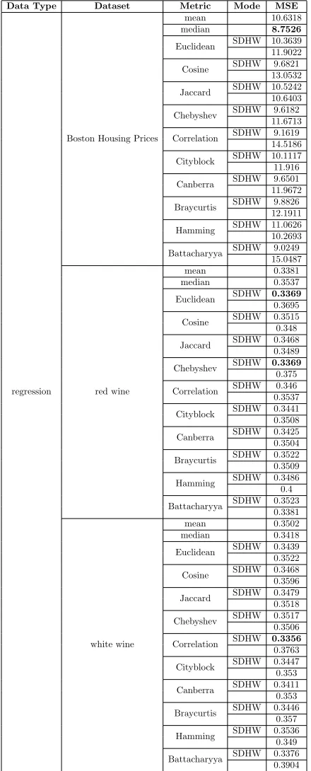
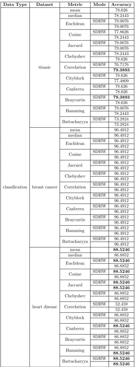
In our experiments, the datasets used for regression are the Boston housing prices dataset from Scikit-learn and the red/white wine quality datasets from the University of California, Irvine (UCI) Machine Learning Repository [ Pedregosa et al. (2011),Cortez et al. (2009)]. The datasets used for classification are the aggregated Titanic dataset from Kaggle1, breast cancer 2 and heart disease 3 datasets from UCI’s Machine Learning repository [ Dua and

1. Obtained from https://www.kaggle.com/heptapod/titanic

(5)

Graff (2017)]. As the objective of the experiments were to illustrate the performance gains in using the distance metrics in the library for ensembling model predictions, the default hyperparameters of each model was used.

The results obtained in our experiments can be found in the Appendix, in Tables 1 & 2 for regression and classification respectively. TheModecolumn indicates which method of assigning weights to a model’s prediction was used. If a value ‘SDHW’ is present, it means that a test involving an assignment of higher weights to predictions with smaller distances was carried out. The error metric used for regression is mean-squared error (MSE) and classification accuracy (accuracy score in Scikit-learn) for the classification task. For experiments excluding the mean and median as metrics, it can be observed that most test cases with ‘SDHW’ in the regression task have lower MSE than those without ‘SDHW’. The results are similar as well for the classification task, though the difference seems much smaller or in many clases negligible.

6. Future Work

The available distance metrics in the library in its initial release are by no means the only ones that can be used in the weighted ensemble. Over time, we will continuously update the library to contain more distance metrics and possibly include additional features that will be beneficial to its users.

Acknowledgments

(6)

Appendix A.

Data Type Dataset Metric Mode MSE

regression

Boston Housing Prices

mean 10.6318 median 8.7526

Euclidean SDHW 10.3639 11.9022 Cosine SDHW 9.6821 13.0532 Jaccard SDHW 10.5242 10.6403 Chebyshev SDHW 9.6182 11.6713 Correlation SDHW 9.1619 14.5186 Cityblock SDHW 10.1117 11.916 Canberra SDHW 9.6501 11.9672 Braycurtis SDHW 9.8826 12.1911 Hamming SDHW 11.0626 10.2693 Battacharyya SDHW 9.0249 15.0487

red wine

mean 0.3381 median 0.3537 Euclidean SDHW 0.3369 0.3695 Cosine SDHW 0.3515 0.348 Jaccard SDHW 0.3468

0.3489 Chebyshev SDHW 0.3369 0.375 Correlation SDHW 0.346 0.3537 Cityblock SDHW 0.3441 0.3508 Canberra SDHW 0.3425 0.3504 Braycurtis SDHW 0.3522 0.3509 Hamming SDHW 0.3486 0.4 Battacharyya SDHW 0.3523

0.3381

white wine

mean 0.3502 median 0.3418 Euclidean SDHW 0.3439 0.3522 Cosine SDHW 0.3468 0.3596 Jaccard SDHW 0.3479 0.3518 Chebyshev SDHW 0.3517 0.3506 Correlation SDHW 0.3356 0.3763 Cityblock SDHW 0.3447 0.353 Canberra SDHW 0.3411

0.353 Braycurtis SDHW 0.3446

0.357 Hamming SDHW 0.3536

0.349 Battacharyya SDHW 0.3376

0.3904

(7)

Data Type Dataset Metric Mode Accuracy

classification

titanic

mean 78.626

median 78.2443

Euclidean SDHW 79.0076

79.0076

Cosine SDHW 77.8626

78.2443

Jaccard SDHW 79.0076

79.0076

Chebyshev SDHW 78.2443

78.626

Correlation SDHW 76.7176

79.3893

Cityblock SDHW 78.626

77.4809

Canberra SDHW 78.626

78.626

Braycurtis SDHW 79.3893

78.626

Hamming SDHW 79.0076

78.2443

Battacharyya SDHW 73.2824

73.2824

breast cancer

mean 96.4912

median 96.4912

96.4912

Cosine SDHW 96.4912

96.4912

heart disease

mean 88.5246

median 86.8852

86.8852

Cosine SDHW 88.5246

86.8852

88.5246

86.8852

52.459

86.8852

88.5246

(8)

References

Richard O. Awichi and Werner G. M¨uller. Improving ssa predictions by inverse distance weighting. 2013.

Veronica J. Berrocal, Adrian E. Raftery, and Tilmann Gneiting. Combining spatial sta-tistical and ensemble information in probabilistic weather forecasts. Monthly Weather

Review, 135(4):1386–1402, 2007. doi: 10.1175/MWR3341.1. URL https://doi.org/

10.1175/MWR3341.1.

Paulo Cortez, Ant´onio Cerdeira, Fernando Almeida, Telmo Matos, and Jos´e Reis. Modeling wine preferences by data mining from physicochemical properties. Decis. Support Syst., 47:547–553, 2009.

Thomas G. Dietterich. Ensemble methods in machine learning. In Multiple Classifier Systems, pages 1–15, Berlin, Heidelberg, 2000. Springer Berlin Heidelberg. ISBN 978-3-540-45014-6.

Dheeru Dua and Casey Graff. UCI machine learning repository, 2017. URL http:// archive.ics.uci.edu/ml.

Jo˜ao Mendes-Moreira, Carlos Soares, Al´ıpio M´ario Jorge, and Jorge Freire De Sousa. En-semble approaches for regression: A survey. ACM Comput. Surv., 45(1), December 2012. ISSN 0360-0300. doi: 10.1145/2379776.2379786. URL https://doi.org/10. 1145/2379776.2379786.

F. Pedregosa, G. Varoquaux, A. Gramfort, V. Michel, B. Thirion, O. Grisel, M. Blon-del, P. Prettenhofer, R. Weiss, V. Dubourg, J. Vanderplas, A. Passos, D. Cournapeau, M. Brucher, M. Perrot, and E. Duchesnay. Scikit-learn: Machine Learning in Python .

Journal of Machine Learning Research, 12:2825–2830, 2011.