Analysis of soil structure interaction of large embedded structure subjected to spatially varying ground motions

(1)

ANALYSIS OF SOIL-STRUCTURE INTERACTION OF LARGE

EMBEDDED STRUCTURES SUBJECTED TO SPATIALLY VARYING

GROUND MOTION

Phuong Tran1, 2_{, Fan Wang}1_{, Didier Clouteau}2

1

_{CEA, DEN, DM2S, SEMT, EMSI}

_{, F- 91191 Gif-sur-Yvette, France ([email protected])}

2 _{MSSMat Lab, UMR 8579 CNRS, Ecole Centrale Paris, F-92295 Châtenay-Malabry, France}

ABSTRACT

This paper aims to present a SSI analysis method for large embedded structures subjected to spatially varying seismic ground motion. The analysis is performed in the time domain. The structure and its nearby soil are modeled by the FE Method. The novelty of the present work is that the seismic loadings applied on the boundary of FE domain is pre-computed on based on a stochastic deconvolution technique and a spectral representation method. This method generates a free field motion inside the soil with given statistical properties on the surface. The advantages of such analyses are that it offers the possibility to simultaneously account for the seismic spatial variability, the non-linear behavior of the structure, the flexibility of its foundation and the effects induced by the embedded foundation.

KEYWORD

:

SSI; seismic spatial variability; stochastic deconvolution; incoherent ground motion.

INTRODUCTION

The SSI analysis with seismic spatial variability has been investigated by earthquake engineering community for several decades. The reference codes one can mention are CLASSIinco-SRSS, SASSI-SRSS and SASSI-simulation (Kassawara et al. 2007). The CLASSIinco-SASSI-SRSS is a computationally efficient tool but it is limited to rigid surface foundations. For structures with flexible or embedded foundation, the SASSI-SRSS or SASSI simulation are required. However, both of these methods are on the basis of sub-structuring methods and the computation is performed in the frequency domain. Hence one cannot account for the non-linearity of the structure. An alternative approach is proposed here to account for both non-linearity of the structure and incoherent ground motion.

The non-linearity of the structures originates from the behavior of the materials or the contact between the foundation and the soil. To account for these non-linear behaviors, the computation must be performed in the time domain and then the Finite Element Methods is a good candidate. It is worth noting that the main difficulties of such analyses are threefold: i) how to consider the seismic input; ii) the unbounded conditions of the FE domain; iii) the computation cost. This work shows the treatment of the seismic input which represents the incoherent free field.

(2)

The novelty of the present approach is that the seismic input is pre-computed by a stochastic deconvolution technique. This method generates a free field motion inside the soil with given statistical properties on the surface. By using an ABCs (Lysmer et al. 1969) at the boundary, a SSI analysis with seismic spatial variability is readily performed.

This paper is outlined as follows. Section 2 reminds the brief description of the seismic spatial variation. The method of generation of incoherent ground motion based on the stochastic deconvolution method (Kausel et al. 1987) and spectral representation method (Shinozuka et al. 1971) is described in section 3. In section 4, validation cases of the proposed approach are presented. Finally, conclusions and perspectives are drawn in section 5.

SEISMIC SPATIAL VARIABILITY

The seismic spatial variability stands the non-uniform ground motion during the earthquake. The causes of seismic spatial variations are diverse; they are related to the fault mechanism, the complex pattern of seismic wave propagation, the variations of site conditions and the wave passage effect.

Assuming the motion at a point x and at time t to be the stochastic process U(x, t), the statistical

properties of the free field can be characterized by the cross-correlation function ( ) between

any two points as follows:

( ) [ ( ) ( )] (1)

where denotes the mathematical expectation.

Under the hypothesis of stationarity, the cross-power spectral density (PSD) can be defined as the Fourier transform of the cross correlation function.

( ) ∫ ( )

(2)

The complex coherency function is a measure of the similarity of the motions at the two different points, it includes both the amplitude spatial variation and the wave passage effects, it is defined as:

( ) ( )

[ ( ) ( )]

(3)

GENERATION OF INCOHERENT FIELD

The details of the method of generation of incoherent ground motion can be found in Tran et al. (2013). This section briefly summarizes this method.

(3)

The extreme case is the one for which the elementary waves are assumed to income from all directions i.e. accounting for all incident angles and azimuthal angles. In such cases, although all elementary waves are assumed to be non-correlated, the motions of the three Cartesian components are correlated. Such cases are termed as full 3D cases. In order to simplify the problem, one only considers the case in which seismic waves propagating in the source-site plane; it means that the azimuthal angle variable is neglected. This hypothesis seems to be reasonable from the engineering point of view. Thus, the horizontal y component of the motion corresponds to the out-of-plane SH waves; the horizontal x and vertical z component of the motions correspond to the in-plane P-SV waves. The x and z components are correlated but they are uncorrelated with the motion in the y direction.

Let ̂( ) be the PSD matrix of the elementary incoming waves at the substratum in the wave-number frequency domain. In general, the elementary incoming waves can be SH, P, and SV waves

which are assumed to be mutually independent random process. Then ̂( ) can be written as

followed:

̂( ) (

̂ ( )

̂ _{( )}

) (4)

where ̂ ( ), ̂ _{( )}_and_̂ _{( )}_{are the power spectrum function of P, SV and SH elementary}

waves.

Let ( ) ( ( ) ( ) ( )) be the displacement vector at point in the

frequency domain. The subscript stands for transposed matrix. ( ), ( ) and ( ) are the

displacement in Ox, Oy and Oz directions respectively. Although the elementary wave are assumed to be

mutually independent, the in-plane motions ( ) and ( ) are correlated because of the inclination

of P-SV incident waves. The in-plane motions and out-of-plane motions are still uncorrelated. The DSP matrix of the ground motion in the wave-number frequency domain on the free surface can be expressed in the following form:

̂( ) (

̂( ) ̂( ) ̂( )

̂ ( ) ̂ ( )

) (5)

where ̂( ), ̂( ) and ̂( ) are the PSD functions in the wave-number frequency

domain of the motions in the Ox, Oy and Oz directions respectively on the free surface.

̂( ) and ̂( ) are the cross PSD functions in the wave-number frequency domain of the in-plane motions on the free surface.

Practically, the statistic properties of the motions are assumed to be known on the free surface and be described by the coherency function as followed:

̂ ( ) ̂ ( ) ( )

̂( ) ̂ ( ) ( )

̂ ( ) ̂ ( ) ( )

(6)

where ̂ ( ) ̂ ( ) and ̂ ( ) are the coherency function in wave-number frequency domain.

(4)

respectively on the free surface. The mentioned descriptions of the statistical properties of the free field are allowed under the assumption of the homogeneity and the stationarity of the ground motion field.

However the cross PSD functions ( ) and ( ) are unknown.

In a layered elastic medium, the relationship between the PSD matrix of the incoming waves and the one on the free surface is established (Kausel et al. 1987):

̂( ) ( ) ̂( ) ( ) (7)

where ( ) is the wave transfer matrix. Taking the 3 diagonal terms of this equation leads to a linear

system to solve for ̂ ( ), ̂ _{( )}_and_̂ _{( )}_.

Once the power spectra of the elementary waves are known, the stationary ground motion can be generated on the basis of spectral representation method (Shinuzoka et al.1971).

SH Waves Propagating Through an Elastic Half-Space Medium

The out-of plane motion in the frequency domain at any point can be computed by the following expression:

( ) ∑ √ ₍₎

( )₍ )

(8)

where is the incident angle with respect to the vertical axis of the jth elementary wave; kxj and kzj are the

horizontal and vertical wave numbers respectively, defined as (

) and

( ) ; is the shear wave velocity of the medium; ₍₎_{is the power spectra of}_jth

elementary SH wave; ( ) is a random variable with a uniform distribution in the interval of [ [.

The PSD function of the elementary waves can be computed from imposed coherency function on the surface by means of the following equation:

₍_{) ̂}

( ) ( ) √ ( ) (9)

where ̂ ( ) is the transformed coherency function in wave-number domain; ( ) is the PSD

function of the out-of-plane motion ( )on the free surface.

The incoherent stationary field is obtained. This free field satisfies the imposed statistic properties on the surface. In order to perform a SSI analysis in the time domain, a non-stationary field is needed.

This field is obtained by normalizing the previous stationary field with a real signal ( ) at the

reference point ( ).

̅( ) ( ) ( )

( ) (10)

The real signal ( ) is selected from data-bases. The selection depends on the objectives of each

analysis. The discussion about this subject can be found in Haselton et al. (2012), Kalkan et al. (2010) and the references therein.

(5)

any point can be considered as the superposition of a set of elementary waves incoming from all directions with random time lag.

VALIDATION OF THE PROPOSED METHOD

The proposed method is validated in 3 steps.

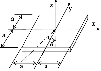
Because this approach is based on the summation of the elementary waves incoming from all directions, the first validation step is the comparison of the response of a square rigid massless foundation subjected to a non-vertically incident SH wave computed by FEMs to the results obtained by Wong and Luco (1978a).

A response of a square rigid massless foundation to non-vertically SH wave in the Oxz plane with

an incident angle is calculated by the FEM performing following step:

- A square rigid massless foundation resting on the elastic half-space is meshed by Finite Elements.

- The traction vector and the velocity at the boundary of the finite element soil mesh are calculated

analytically on the basis of the solution of the wave propagation equation in the half-space.

- A Lysmer’s absorbing condition is used to satisfy the radiation condition.

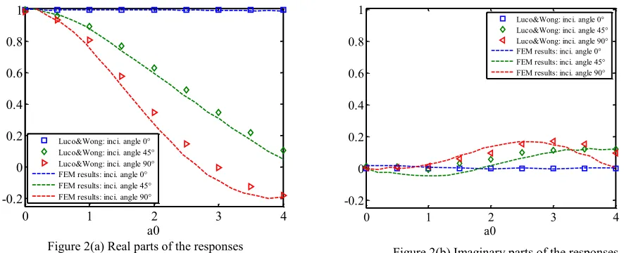
The responses are complex functions of the dimensionless frequency and of the incident

angle . Figure 2 and 3 show the real and imaginary parts of the results obtained by Wong et al. (1978a)

and the ones obtained by FEM in the case of a half-space with a Poisson’s ration for different

incident angles.

The second step of the validation is the comparison of the response of a square rigid massless foundation subjected to an incoherent seismic loading in the cases of an isotropic coherency function and an anisotropic coherence function. The coherency function taken is

( ) [ ( ) ] (11)

where is equal to 0.0002 s/m in this example. In the isotropic case √ and in the

anisotropic one . In the case of plane waves propagating from the source to the site, the coherency

function depends only on the distance of separation projected on the propagation direction, the anisotropic model of coherency function is more suitable. Figure 4 shows the amplitude of the transfer function between the free field ground motion and the foundation response being function of the dimensionless

frequency . This analysis is carried out using Luco and Wong’s (1986) method which is implemented

in the Cast3m code (Wang et al. 1995).

𝜽

y

z

x

a

(6)

Figure 2(a) Real parts of the responses

Figure 3(a): Real parts of the responses Figure 3(b): Imaginary parts of the responses

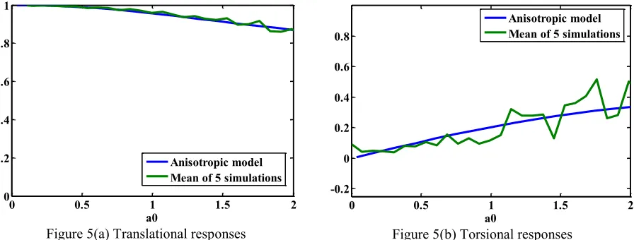
The final step of validation is the comparison of the results obtained by our approach and the one obtained by Luco and Wong (1986) method. Figure 5(a) shows the transfer function between the power spectral density of the translational response components with the corresponding component of the free-field ground motion. The blue curve is the result obtained by Luco and Wong method. The green curve is the mean of five simulations. Figure 5(b) presents the amplitude of transfer function between the motions along y axis and the normalized torsion response about the z axis.

0 1 2 3 4

-0.2 0 0.2 0.4 0.6 0.8 1 a0

Luco&Wong: inci. angle 0° Luco&Wong: inci. angle 45° Luco&Wong: inci. angle 90° FEM results: inci. angle 0° FEM results: inci. angle 45° FEM results: inci. angle 90°

0 1 2 3 4

-0.2 0 0.2 0.4 0.6 0.8 1 a0

0 1 2 3 4

-0.2 0 0.2 0.4 0.6 0.8 1 a0

0 1 2 3 4

-0.2 0 0.2 0.4 0.6 0.8 1 a0

Figure 2(b) Imaginary parts of the responses

Figure 2: Translation responses of a square rigid foundation to non-vertically incident SH waves.

(7)

Figure 4(a) Translational

responses

Figure 4(b) Torsional responses

Figure 4: Amplitude of the transfer function between the free field ground motion and the foundation responses.

Figure 5(a) Translational responses Figure 5(b) Torsional responses

Figure 5: Amplitude of the transfer function between the free field ground motion and the foundation responses.

CONCLUSIONS

A novel approach for SSI analyses with the spatial variability is shown. This approach is classified as the global method where the structure and the soil are meshed by FEs. The dynamic equations are solved in the time domain. The seismic loadings are pre-computed and applied on the boundary of soil mesh. These seismic loadings represent the variability of far-field incident waves. The results obtained by this approach in the case of a rigid square foundation resting on an elastic half-space are comparable to the reference.

The advantages of this approach are that one can perform a SSI analysis with the spatial variability in the time domain. That allows accounting for the non-linearity of the structure and the flexibility of the foundation. Moreover, in order to account for the spatial variability, it only requires a

0 1 2 3 4

0 0.2 0.4 0.6 0.8 1

a0

Isotropic model Anisotropic model

0 1 2 3 4

0 0.2 0.4 0.6 0.8 1

a0

Isotropic model Anisotropic model

0 0.5 1 1.5 2

0 0.2 0.4 0.6 0.8 1

a0

Anisotropic model Mean of 5 simulations

0 0.5 1 1.5 2

-0.2 0 0.2 0.4 0.6 0.8

a0

(8)

signal at a reference point and the coherency function on the ground surface which is usually used in practical engineering. It is simple to implement in an existing FE code.

The main classical drawback of this approach is the computation cost. In order to satisfy the radiation condition, the Lymer’s condition is used. However, according to our experience, the dimension of soil mesh must be about 5 times larger than the dimension of the foundation.

Our future works aim to extend the approach to the case of P-SV waves and the stratified soil medium.

REFERENCES

Basu, U., and Chopra, A. K. (2003). “Perfectly matched layers for time-harmonic elastodynamics of

unbounded domains: the theory and finite-element implementation”, Comput. Methods. Appl.

Mech. Engrg. 192 (2003) 1337-1375.

Haselton, C.B., Whittaker, A.S., Hortacsu, A., Baker, J.W. and Bray J.W. (2012). “Selecting and Scaling

Earthquake Ground Motions for Performing Response-History Analyses,” Proceedings of Fifteenth

World Conference on Earthquake Engineering, Lisboa, Portugal.

Kalkan, E., and Chopra, A.K. (2010). “Practical Guidelines to Select and Scale Earthquake Records for

Nonlinear Response History Analysis of Structures,” U.S Geological Survey Open-File Report,

113p.

Kassawara, R., and Sandell, L. (2007). “Program on Technology Innovation: Effects of Spatial

Incoherence on Seismic Ground Motions”, Electric Power Research Institute Report.

Kausel, E., and Pais, A., (1987). “Stochastic Deconvolution of Earthquake Motions”, Journal of

Engineering Mechanics, 113(2): 266-277.

Luco, J. E., and Wong, H.L. (1986). “Response of a Rigid Foundation to a Spatially Random Ground

Motion”, Earthquake engineering and structural dynamics, vol. 14, 891-908.

Lysmer, J., and Kuhlemeyer, G. (1969). “Finite Dynamic Model for Infinite Media”, ASCE, vol. 95, EM4,

pp. 859-877.

Shinozuka, M., and Jan, C.-M. (1972). ‘Digital Simulation of Random Process and Its Applications”, Journal of Sound and Vibration, 25(1): 111-128.

Tran, Ph., Wang, F., and Clouteau, D. (2013). “Generation of Incoherent Ground Motions for SSI

applications”, Procs. of 4th International Conference on Computational Methods in Structural

Dynamics and Earthquake Engineering, Kos Island, Greece.

Wang, F., and Gantenbein F. (1995). “Calculation of Foundation Response to Spatially Varying Ground

Motion by Finite Element method”, Procs. of 13th Conference on Structural Mechanics in Reactor

Technology, Porto-Alegre, Brasil.

Wolf, J.P., and Song, Ch. (1996). Finite-element Modelling of Unbounded Media, ISBN 0-471-961345, Published by John Wiley & Sons.

Wong, H.L., and Luco J.E. (1978a). “Dynamic Response of Rectangular Foundations to Obliquely