APPLICATION OF CFD BASED ATMOSPHERIC DISPERSION MODEL
FOR THE SITE WITH COMPLEX TOPOGRAPHY
R.B. Oza*, Indumati S.P., M.B. Pote and V.D. Puranik
Environmental Assessment Division, Bhabha Atomic Research Centre, Mumbai, INDIA-400085 *E-mail of corresponding author: [email protected]
ABSTRACT
One of the serious problems in applying CFD based model for atmospheric flow field simulation is the initialization of the model, especially for complex topography, where the flow field is expected to be inhomogeneous. In our study, the CFD based PANEPR model was initialized with different combinations of meteorological measurements carried out at two different locations. Total five scenarios were considered: (a) using only vertical profile of meteorological data collected at Gamma Garden (GG), BARC, using SODAR (b) using only single point measurement at South Site (SS), BARC, using wind vane and cup anemometer, (c) using profile of the data at GG and single point measurement at SS, (d) using profile data at GG and synthetic profile generated for SS using interpolation/extrapolation technique, and (e) using profile data at GG + Single point data at SS + assigning the same value of meteorological parameter beyond 250 m altitude for the SS as those of the GG. The results of the study indicate that the flow field generated using CFD based model significantly depends on the number of measurement locations, on the locations of measurement, and on the way in which data at measurement locations are interpolated/extrapolated. Additionally, the model was also applied to study the effect of topographic structure, such as an isolated hill. This parametric study on the effect of presence/absence of a hill on atmospheric dispersion of pollutant suggest that the elevated terrain may increase the ground level concentration of pollutant in the nearby areas, however, it also enhances the dispersion of pollutant and may reduce the ground level concentration for far away locations.
INTRODUCTION
Computational Fluid Dynamics (CFD) is considered to be an effective tool for the problems that involve fluid flow. This is because of the versatile nature of the equations involved to accommodate domain specific phenomena. Though CFD is considered to be a useful technique for the fluid flow problems, its application to atmospheric fluid flow has remained limited because of the huge computational power and the large domain size requirements of the atmospheric flow problems. Due to the recent advent of fast computational facility, it has now become possible to apply CFD based techniques to atmospheric flow problems. In our developmental studies, the CFD based model PANEPR [1, 2] developed by fluidyn, Transoft, Bangalore, was modified to incorporate Numerical Weather Prediction (NWP) Model MM5 data for atmospheric dispersion and radiological impact assessment studies. The present paper describes the parametric studies carried out using PANEPR model for the
Trombay site, including the effect of complex topography. The model was used with k- as the turbulence closure
scheme.
CASE STUDY
Importance of multiple meteorological measurement stations and their locations in atmospheric dispersion of pollutant for complex topography
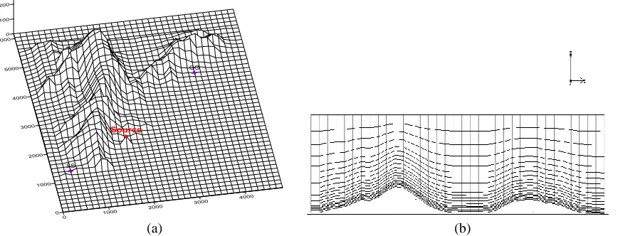
beyond 250m height at SS as those of GG and allowing model to generate interpolated wind field for intermediate heights. The domain consists of 36, 46 and 20 Cartesian grid points in East (model X-coordinate), North (model Y-coordinate) and Vertical (model Z-Y-coordinate) directions respectively. The digital elevation information for the site was available at 134m resolution, and hence uniform grid spacing of 134m was used for the horizontal directions covering an area of 4.8 km x 6.1 km. The grids in vertical direction were kept at unequal interval, with finer resolution closer to the ground and coarse resolution at the model top. The PANEPR model makes use of terrain following coordinate system to take into account terrain elevation information for flow field as well as dispersion estimation. The horizontal grid structure alongwith the locations of the source and meteorological stations and vertical grid structure in XZ cross section (Y = 36) generated over Trombay site are shown in Fig. 1 (a) and (b) respectively.
(a) (b)
Fig. 1 (a) XY grid structure using terrain following coordinate system (b) XZ cross section of grid structure using terrain following coordinate system (Y=36).
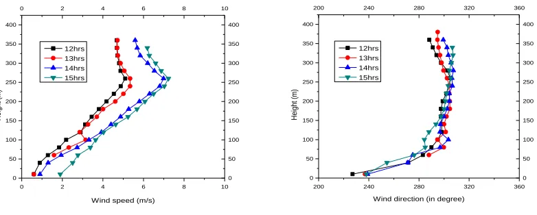
Simulations with PANEPR model was carried out for May 23, 2006 for 4 hours starting from 12:00 hrs to 15:00 hrs for the scenarios described above. However, the results of only 12:00 hrs are presented here. The wind speed and wind direction recorded by the SODAR at GG and with cup anemometer and wind-vane at SS are shown in Fig. 2 (a) and (b) respectively for the time period of interest. The meteorological data were measured at an interval of 60 minutes, and were fed to the model at the same interval. It is to be noted that meteorological data averaged over a period is stored at the end of averaging period and hence data at 12:00 hrs represents data averaged between 11:00 hrs and 12:00 hrs. Thus, model dispersion estimate at 12:00 hrs, is the result of meteorological conditions prevailing between 11:00 hrs and 12:00 hrs. To study the atmospheric dispersion of pollutant, a hypothetical source location was assumed somewhere nearer to DHRUVA & CIRUS reactor with release height of 100m, and continuous release rate of 1 g/s for passive tracer.
0 50 100 150 200 250 300 350 400
0 2 4 6 8 10
0 50 100 150 200 250 300 350 400
0 2 4 6 8 10
Gamma Garden Data
South Site Data
Wind speed (m/s)
H e ig h t (m) 12hrs 13hrs 14hrs 15hrs 0 50 100 150 200 250 300 350 400
200 250 300 350
Direction (in degree)
H e ig h t (m) 12hrs 13hrs 14hrs 15hrs
South Site Data
Gamma Garden Data
0 50 100 150 200 250 300 350 400
200 250 300 350
As can be seen from Fig. 2(a), the wind speeds measured by the SODAR at various altitudes are significantly higher as compared to the wind speed recorded at SS. Figure also shows that wind speed at both the locations strengthens with time, which is normally expected in the afternoon hours. The wind directions at different time period for both the locations are shown in Fig. 2(b). The predominant wind direction at GG at almost all the altitudes is WNW to NW, whereas at the SS it is SW to WSW. Thus, wind speed and wind direction conditions at these two locations are significantly different. The potential release point, DHRUVA and CIRUS reactors, is somewhere nearer to the line joining both the meteorological stations and is more nearer to SS compared to Gamma Garden. And hence, in the absence of meteorological measurements in between, the meteorological conditions around the potential release point is expected to get influenced by the measurements carried out at both these stations, with relatively higher weightage to SS station as it is nearer compared to GG
The meteorological data shown in Fig. 2(a) and (b) are used for the scenarios (a) to (c) mentioned earlier. In order to generate vertical profile for SS, it was assumed that even though there is a significant speed as well as directional shear between the two meteorological measurement locations, the upper air data may not show such spatial variations and hence could be assumed to remain same at both the locations. Keeping this in mind, the wind speed and direction data collected at SS were converted into u and v components and were extrapolated in the vertical direction using
(1)
where Zr is the reference height where measurements are carried out (10m in this case), uzr is the reference
u-component of wind at the reference height, Z is the height in vertical where extrapolated u-components are required, uz
is the extrapolated wind component at height Z, and p is the wind extrapolation parameter (taken as 0.11 in this case, based on unstable atmospheric conditions). Similarly, v-components were extrapolated. The components were extrapolated for the same vertical levels of SODAR measurements up to a height of 250m and above this, the SODAR profiles were assumed to prevail at SS also. After estimating u and v components at various altitudes for SS, these data were weighted with respect to SODAR data in the following manner.
(2)
where ussz is extrapolated/interpolated wind component at height Z for south site, uz is the earlier extrapolated wind
component at SS for height Z, uzsodar is the u component of wind speed at height Z for SODAR measurement, and
is the weighting parameter, which is equal to 0 for the reference measurement height Zr and 1 for Z 250m (linearly
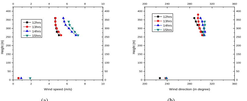
interpolated between the two). Thus, this interpolation scheme will give higher weightage to SS data for lower altitude whereas higher weightage to SODAR data for higher altitudes. The synthetic profiles thus generated for SS station are shown in Fig. 3(a) and (b) for wind speed and wind direction respectively. As expected, the profile generated at SS shows significant speed as well as directional shear. Similarly, the meteorological data used for SS in case of scenario (e) are shown in Fig. 4(a) and (b).
0 50 100 150 200 250 300 350 400
0 2 4 6 8 10
0 50 100 150 200 250 300 350 400
0 2 4 6 8 10
Wind speed (m/s)
H ei gh t (m) 12hrs 13hrs 14hrs 15hrs 0 50 100 150 200 250 300 350 400
200 240 280 320 360
0 50 100 150 200 250 300 350 400
200 240 280 320 360
Wind direction (in degree)
H e ig h t (m) 12hrs 13hrs 14hrs 15hrs
(a) (b)
0 50 100 150 200 250 300 350 400
0 2 4 6 8 10
0 50 100 150 200 250 300 350 400
0 2 4 6 8 10
Wind speed (m/s)
H e ig h t (m) 12hrs 13hrs 14hrs 15hrs 0 50 100 150 200 250 300 350 400
200 240 280 320 360
0 50 100 150 200 250 300 350 400
200 240 280 320 360
Wind direction (in degree)
H e ig h t (m) 12hrs 13hrs 14hrs 15hrs
(a) (b)
Fig. 4: (a) Wind speed profiles used for South site where surface winds are taken from South site data and upper air data are taken from SODAR (b) Wind direction profiles for the same.
The methodology followed in PANEPR model for generating flow field as well as atmospheric dispersion of pollutant is broadly as follows:
1.Interpolate/Extrapolate the wind field in horizontal directions based on the measured meteorological data using inverse square relation for the distance between measurement point and the point at which values are being estimated.
2.Interpolate/extrapolate the wind field in vertical direction, either from the measured data, or by power law profile.
3.The interpolated wind field is subjected to mass consistency.
4.Use mass consistent wind field to initialize the model and also for fixing the boundary conditions.
5.Solve for mass, momentum and energy conservation.
6.Use the wind field generated in previous step for solving Advection Diffusion Equation.
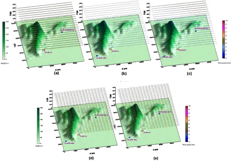
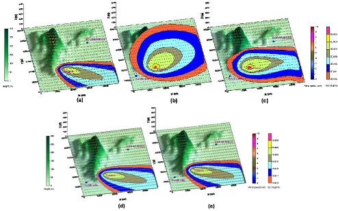
As is clear from Step-1, the interpolated wind field is influenced by the nearness of the measurement location as it depends on the inverse square of the distance. The wind field generated by PANEPR model at 10m height above the topography for 12:00 hrs for the cases (a) to (e) described earlier are shown in Fig. 5(a)-(e). Similarly, the wind field generated by the model at 400m altitude above the ground is shown in Fig. 6(a)-(e) for the same period. The ground level concentration values estimated by the model under the five different scenarios for 12:00 hrs are shown in Fig. 7(a)-(e).
at lower altitude are significantly getting affected by the strong winds at higher altitude, because of the momentum transfer. Under such cases, the CFD based solutions wipe out the initial conditions supplied to the model based on observations. Thus, proper care should be taken while supplying the data to CFD based models depending upon the case.
The model generated wind fields at 400m altitudes are given in Fig. 6(a)-(e) for the same case. As can be seen, the wind speed increases with the altitude, however, the general trend remains same as their respective flow fields at 10m altitude. Ideally, the upper level wind should not get affected by the measured data at lower altitude, however, since the wind field first gets horizontally interpolated and then vertically, the lower wind speed over south site affects the wind speed even at an altitude of 400m due to vertical interpolation (Fig.7(c)). It is worthy to mention here that the scenarios (d) and (e) were generated in view of this discussion. However, as discussed earlier, these scenarios generate flow fields which are independent of the measurements carried out at lower altitude and are mainly governed by the driving flow field at higher altitude. The isopleths of ground level concentration for all the five scenarios are given in Fig. 7(a)-(e). In general the surface isopleths follows the wind flow patterns, as expected. Additionally the figures also show that when wind speed weakens (e.g., scenario (b) and (c)), diffusion becomes dominant as compared to transport and gives broadened isopleths of concentration distribution over the ground. The lower wind speed also gives rise to higher concentration values as shown in Fig. 7(b) and (c).
Thus, this study suggests that the flow field generated using CFD based model gets significantly affected by the number of measurement locations, by the locations of measurements and also by the way in which data are interpolated/extrapolated for the measurement locations. As it is observed from the case studies, the data from a single point measurement location (South site) and vertical profile at other location (Gamma garden), i.e., scenario (c) considered in our case study, generates a flow field that is consistent with the measurements at both the locations. But this scenario maintains nearly the same horizontal speed and directional shear for higher altitude as observed for lower altitude, and this seems to be unrealistic for those altitudes. However as ground level concentration of pollutant is affected by the lower altitude wind field only, this method seems to work reasonably well. Though it should be kept in mind that model initialization procedure strongly depends on the distance between measurement location and the point at which interpolated data are required. Hence, in this, the nearness of the measurement location may govern the flow field in the source area, even if the measurement location is not representative. On the other hand, if upper level data are assumed to remain same for the measurement locations, they not only govern the upper level flow field but also starts influencing the surface level flow field (i.e., scenarios (d) and (e) considered here). Thus, in this method the surface level measurements lose its importance.
Fig. 5: Wind field generated by PANEPR at 10m above topography for scenarios (a) to (e) at 12:00 hrs.
Fig. 7: Ground level concentration estimated by PANEPR for scenarios (a) to (e) at 12:00 hrs.
Effect of hill behind plutonium plant on atmospheric dispersion of pollutants
Blocking effects generated by topographical features is one of the dominant causes of distortion of atmospheric flow field. Blocking effects due to terrain elevation leads to complex flow patterns that might generate mean concentration distributions significantly different from those that might be expected from the mean flow in the absence of the complex terrain features for atmospheric dispersion of pollutants. The hilly terrain surrounding the Trombay site can affect the flow field in a similar way and can in turn affect the ground level concentration on the lee side of the hills. Modeling the wind flow around an isolated hill helps to develop an understanding of the flow in real terrain. On these lines, the effect of an isolated hill on the wind flow at the Trombay site was studied. In order to study the effect of the modified wind field on atmospheric dispersion of pollutant, the ground level concentration distribution was also examined for a hypothetical release scenario as discussed in previous case.
(a) (b)
Fig. 8: Ground elevation data used for model simulation (a) with PP hill (b) without PP hill
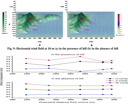
The horizontal wind field at the first model level for the cases simulated is shown in the Fig. 9(a) and (b). As is clearly seen from the Fig. 9(a), the surface winds are blocked by the hill and there is a deflection of wind to the east side in the lower levels. This also leads to deceleration of the wind in the upwind side of the hill whereas wind gets speeded up at the top of the hill and behind the hill there is deceleration. In the absence of hill, flow remains uniform in the downwind direction. These findings are also depicted in the plot of variation of the U, V and W components of wind in the downwind direction in Fig. 10. In the absence of the hill, the flow is dominated by the V component of velocity and is almost uniform whereas in the presence of hill, the components get modified and leads to a different flow pattern. Similarly, the W-component is practically absent in the absence of hill. Because of the blocking effect provided by the hill, there is an upslope and downslope flow present on the windward and leeward side of the hill. After nearly 2 km from the source, the surface flow becomes uniform again indicating that the flow is no more affected by the presence of hill.
The effect of the terrain induced flow field can be directly seen on the distribution of ground level concentration as well. Fig.-11 is the plot of ground level concentration in the downwind direction in the presence and absence of the hill. The concentration values at and after the location of the hill are consistently higher than the corresponding values in the absence of the hill. This is because in the presence of hill, the elevated surface is in fact at higher elevation (130 m) compared to plume centerline (100 m), and hence higher concentration values are observed above the hill surfaces. Beyond the hill, since the plume has already impacted over the hill surface, it will further disperse like a ground level release. This is also confirmed by the negative vertical velocity observed on the lee side of the hill. Thus the presence of hill is expected to increase ground level concentrations in the nearby areas due to the nearness of the elevated surface to the plume centre-line and also because of the modification in the flow field. However, the spread in ground level concentration distribution shown in Fig.11 also suggests that the presence of hill provides additional dilution to the released pollutant and is expected to reduce ground level concentration for far away distances. The results presented here are only indicative, as it was found in our study that the turbulence model used in PANEPR model is insensitive to temperature profile, and moreover, the eddy-diffusivity estimated by the model is significantly lower as compared to the eddy-diffusivity observed in other modeling systems. In view of this, the results stated here are qualitative and no quantitative conclusion can be made.
Fig. 9: Horizontal wind field at 10 m (a) in the presence of hill (b) in the absence of hill
1000 1500 2000 2500 3000 3500 4000 4500
-0.2 0.0 0.2 0.4 0.6 0.8 1.0
1000 1500 2000 2500 3000 3500 4000 4500
-0.2 0.0 0.2 0.4 0.6 0.8 1.0
In the absence of hill
Wi
nd
co
mp
on
en
ts
(m/
s)
In the presence of hill
U-comp V-comp W-comp
Downwind distance from source (m)
Fig. 10:Variation of U,V and W components of wind at 10 m level as a function of downwind distance from source
(a) (b)
Fig. 11: Ground level concentration (a) in the presence of hill (b) in the absence of hill
500 1000 1500 2000 2500 3000 3500 4000 4500 5000 5500 6000
Y
(
m
)
500 1000 1500 2000 2500 3000 3500 4000 4500
X (m)
500 1000 1500 2000 2500 3000 3500 4000 4500
1E-012 1E-011 1E-010 2E-010 3E-010 4E-010
Conc (kg/m3)
0.1 40 80 120 160 200 240 280 320
CONCLUSION:
The study suggests that the flow field generated using CFD based model significantly depends on the number of measurement locations, on the locations of measurements, and on the way in which data at measurement locations are interpolated/extrapolated. It was observed in this study that for a better utilization of the CFD based software for atmospheric dispersion studies, it is better to have more measurements near to the source area as well as in the areas in which impact of the released pollutant could be important. The parametric study on the effect of presence/absence of a hill on atmospheric dispersion of pollutant suggested that elevated terrain may increase the ground level concentration of pollutant in nearby areas, however, it also enhances dispersion of pollutant and may reduce the ground level concentration for far away locations.
REFERENCES
[1] Oza, R.B., Puranik, V.D., Kushwaha, H.S., Krishna Prasad, Arun Murthy, Dispersion of radionuclides and radiological dose computation over a mesoscale domain using weather forecast and CFD model, International conference on CFD4NRS-3, USA, September, 2010.