A New Non-linear Multistep Method Based on Centroidal Mean
in Solving Initial Value Problems
1Nazeeruddin Yaacob & Teh Yuan Ying
Department of Mathematics, Faculty of Science, Universiti Teknologi Malaysia 81310 UTM Skudai, Johor, Malaysia
e-mail:1[email protected]
Abstract A new 2-step fourth order implicit non-linear multistep method based on centroidal mean is considered in this paper. The new method is tested on some test problems; and numerical results show that the new method is able to produce accept-able numerical solutions for these test problems. Comparisons in terms of numerical accuracy between the new method and the classical 2-step Adams-Moulton method are carried out as well. Numerical experiments show that our new method performs better than the classical 2-step Adams-Moulton method in solving these test problems.
Keywords Initial value problems, non-linear multistep method; centroidal mean; Adams-Moulton method; 3-stage fourth order Lobatto IIIC method.
1
Introduction
Numerical methods from the class of linear multistep methods and the class of Runge-Kutta methods are defined by [1]
k
X
j=0
αjyn+j =h k
X
j=0
βjfn+j (1)
and
yn+1=yn+h s
P
i=1
biki
ki=f tn+cih, yn+h s
P
j=1
aijkj
!
, i= 1,2, . . . , s.
(2)
respectively. These methods are among the most common used numerical methods for the first order initial value problem of the form
y0(t) =f(t, y(t)), y(a) =y0, t∈[a, b]. (3)
A new research trend had emerged around the 1990’s where researchers start to incorporate mean expressions into linear Kutta method in (2) to form a new kind of Runge-Kutta method that based on different kinds of means. This special type of Runge-Runge-Kutta method is considered as non-linear method due to the non-linear structures that arise from the implementation of various mean expressions. Articles which have discussed this type of method are such as [3] through [28].
organized as follows: In section 2, we present the procedure for obtaining the new 2-step implicit non-linear method based on centroidal mean. In Section 3, we present the local truncation error, consistency, zero-stability and convergence analysis of the new method. The stability polynomial and the regions of absolute stability for the new method are presented in Section 4. Section 5 shows the numerical implementations of the new implicit method to a variety of test problems and compares its performance with the classical 2-step implicit Adams-Moulton method in terms of numerical accuracy. Some remarks and conclusions will be given in Section 6.
2
Derivation of the 2-step Implicit Non-linear Method Based on
Centroidal Mean
Firstly, we define the new 2-step implicit method as
α2yn+2+α1yn+1+α0yn =h
c1fn+2+c2fn+1+c3fn+c4 2(f2
n+2+fn+2fn+1+fn2+1)
3(fn+2+fn+1)
+c5 2(f2
n+1+fn+1fn+f 2 n)
3(fn+1+fn) +c4
2(f2
n+2+fn+2fn+f 2 n)
3(fn+2+fn)
(4)
where α0= 0,α1=−1,α2= 1 withc1,c2, c3,c4,c5 andc6 are constants that need to be determined. Note thatfn+2+fn+16= 0,fn+1+fn6= 0 andfn+2+fn 6= 0. On using Taylor series to expand both sides of equation (4) up to O h4, and compare each coefficient, we obtain the following equations:
c1+c2+c3+c4+c5+c6= 1, (5)
2c1+c2+ 3 2c4+
1
2c5+c6= 3
2, (6)
2c1+ 1 2c2+
5 4c4+
1
4c5+c6= 7
6, (7)
1 12c4+
1 12c5+
1
3c6= 0, (8)
−1 8c4−
1 24c5−
1
3c6= 0, (9)
1 4c4+
1 12c5+
2
3c6= 0. (10)
Using MATHEMATICA 5.0 in solving the system of equations given in (5) – (10), we obtain a set of solutions in terms of a free parameterc6 shown as follows:
c1= 5 12+
c6
2, c2= 2
3+ 2c6, c3=− 1 12+
c6
2, c4=−2c6, c5=−2c6.
On substituting theseci,i= 1,2, . . . ,6 andα0= 0,α1=−1,α2= 1 into equation (4), the resulting method is a 2-step implicit non-linear method based on centroidal mean:
yn+2−yn+1=h 125 +c26fn+2+ 32+ 2c6fn+1+ −121 +c26fn + (−2c6)
2(f2
n+2+fn+2fn+1+fn2+1)
3(fn+2+fn+1) + (−2c6)
2(f2
n+1+fn+1fn+f 2 n)
3(fn+1+fn) +c6
2(f2
n+2+fn+2fn+f 2 n)
3(fn+2+fn)
Method (11) is named Non-linear Multistep method based on centroidal mean of two steps and fourth order or shortly NLMMCeM(2,4). The local truncation error in terms ofc6for NLMMCeM(2,4) is given by
h4 −1 24f 000 n
+h5 c6(f
0
n) 4
12 (fn)3
−c6(f 0
n) 2
f00
n 12 (fn)2
+c6(f
00
n) 2
12fn
− 17 360f
(4) n
!
+O h6. (12)
Since there is a free parameter c6, we choose this parameter so that the local truncation error shown in (12) is inO h6
. From (12), we force the first two terms to zero that is
h4 −1 24f 000 n
+h5 c6(f
0
n) 4
12 (fn)3
−c6(f 0
n) 2
f00
n 12 (fn)2
+c6(f
00
n) 2
12fn
− 17 360f
(4) n
!
= 0. (13)
After some algebraic manipulations,c6 is obtained as follows:
c6=
(fn)
3
15f000
n + 17hf (4) n
30h(f0
n) 4
−fn(fn0) 2
f00
n + (fn) 2
(f00
n)
2 (14)
where (f0
n) 4
−fn(fn0) 2
f00
n + (fn)2(fn00) 2
6
= 0. Note thatc6 is a constant since all functions
fn+j(i) , i= 0,1,2,3,4,5are evaluated at the pointtn. Therefore, the local truncation error for NLMMCeM(2,4) withc6in (14) is given by
LTE (Centroidal) = h 5 720 − 2
3f0
n
(f0
n) 2
−fnfn00
2
+ (fn)
2
(f0
n) 2
−2fnfn00
f000
n
15f000
n + 17hf (4) n
fn
(f0
n) 4
−fn(fn0) 2
f00
n+ (fn)2(fn00) 2
−h6
7
240f (5) n
+O h7
. (15)
3
Consistency, Stability and Convergence Analysis for
NLMM-CeM(2,4)
We extend the theory of consistency, zero-stability and convergence for the linear multistep method to the new method NLMMCeM(2,4). As usual, the first characteristic polynomial,
ρ(ζ) and the second characteristic polynomial of NLMMCeM(2,4), σ(ζ) can be obtained from the left-hand side and right-hand side of equation (11) respectively; with the substi-tution ofyn+j =fn+j =ζj andfn+j(i) =ζj for i= 0,1,2,3,4,5 andj = 0,1,2. Therefore, we obtain
ρ(ζ) =ζ2−ζ (16)
and
σ(ζ) = 5
12+
c6
2
ζ2+ 2 3+ 2c6
ζ+ −1
12+
c6
2
+ (−2c6)
2“(ζ2)2+ζ2 ×ζ+ζ2” 3(ζ2+ζ)
+ (−2c6)
2(ζ2+ζ×1+12)
3(ζ+1) +c6
2“(ζ2)2
+ζ2×
1+12”
3(ζ2+1)
From the assumption fn+j(i) =ζj fori = 0,1,2,3,4,5, we note that c
6 in (14) is evaluated
at the point tn and therefore we havefn(i) =ζ0 = 1 fori= 0,1,2,3,4,5. On substituting
fn(i)=ζ0= 1 fori= 0,1,2,3,4,5 into equation (14) yield
c6=
13
(15 (1) + 17h(1))
30h(1)4−1×(1)2×1 + (1)2(1)2
= 15 + 17h 30h .
The first derivative of equation (16) is
ρ0(ζ) = 2ζ−1. (18)
On substitutingζ= 1 into equations (16), (17) and (18) we obtain the following results:
ρ(1) = 0, σ(1) = 1 and ρ0(1) = 1. (19)
Since conditions in (19) hold for NLMMCeM(2,4), then we can say that it is consistent. To determine the zero-stability of NLMMCeM(2,4), we must make sure that no root of
ρ(ζ) has modulus greater than one, and every root with modulus one is simple. Therefore, from (16), the roots of
ζ2−ζ= 0
are ζ1= 1 and ζ2 = 0. Consequently, we have|ζ1|= 1 and|ζ2|= 0 which are not greater than one and simple. In view of this, we can say that NLMMCeM(2,4) is zero-stable.
Finally, we can claim that NLMMCeM(2,4) is convergent because it is shown to be consistent and zero-stable.
4
Absolute Stability of NLMMCeM(2,4)
In order to carry out the stability analysis for NLMMCeM(2,4), we must obtain the stability polynomial and its corresponding regions of absolute stability. We can obtain the stabil-ity polynomial of NLMMCeM(2,4) by applying the Dahlquist’s test equation y0 = λy to
equations (11) and (14) [2]. Note that λis a complex constant with negative real part. On substituting (14) into (11) and then substituting fn+2=λyn+2, fn+1 =λyn+1, fn =λyn,
f0
n=λ2yn,fn00=λ3yn,fn000=λ4yn,fn(4)=λ5yn,yn+2=ζ2,yn+1=ζand yn= 1 into (11), we obtain the following stability polynomial for NLMMCeM(2,4) as follows:
(195−58z)ζ4−(240 + 188z)ζ3+ (270 + 42z)ζ2−(240 + 188z)ζ+ (15 + 32z) = 0 (20)
Figure 1: Stability Region of NLMMCeM(2,4)
5
Numerical Experiments and Comparisons
In this section, NLMMCeM(2,4) is used to solve some test problems in order to check its reliability and accuracy. We present i) the maximum absolute error over the integration interval given by
max
0≤n≤N{|y(tn)−yn|}
where N is the number of integration steps; and ii) the absolute error at the end-point of integration interval given by|y(tn)−yN|for each test problem. Note thaty(tn) represents the exact solution of a test problem at pointtn, whileyn is the approximations of the exact solution at pointtn of a test problem. The notation 1.26681(-5) indicates 1.26681×10⁻⁵. Numerical results obtained using NLMMCeM(2,4) is compared with the numerical results obtained using the classical 2-step implicit Adams-Moulton method given by [29]
yn+2−yn+1=h
5
12fn+2+ 2 3fn+1−
1 12fn
(21)
where the local truncation error of (21) is
LTE (Adams−Moulton) =h4
−1
24f
000
n
+h5
−17
360f (4) n
+O h6
. (22)
0 1
6 −
1 3
1 6 1
2 1 6
5
12 −
1 12
1 1
6 2 3
1 6 1
6 2 3
1 6
Problem 1: [17]
y0(t) =y(t)−t2+ 1, y(0) = 1
2, t∈[0,1]. The exact solution for Problem 1 is given byy(t) = (t+ 1)2−1
2e t.
Problem 2: [24]
y0(t) =y(t) cost, y(0) = 1, t∈[0,1].
The exact solution for Problem 2 is given byy(t) =esin(t).
Problem 3: [31]
y01(t) = 0.2y2(t), y1(0) = 1,
y20 (t) =−0.2y1(t), y2(0) = 1.
Problem 3 is solved numerically over the integration intervalt∈[0,1] and the exact solutions for Problem 3 are given byy1(t) = cos 0.2t+ sin 0.2tandy2(t) =−sin 0.2t+ cos 0.2t.
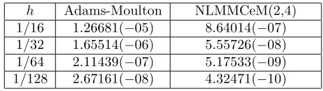
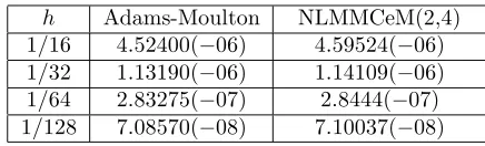
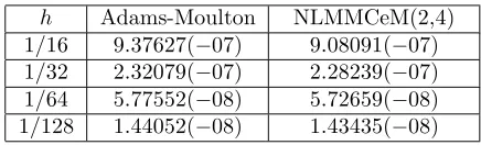
Table 1 to Table 8 show that NLMMCeM(2,4) has no difficulty in solving all the test problems mentioned above; and it performs better than 2-step Adams-Moulton for different step length for Problem 1 and Problem 2. On the other hand, NLMMCeM(2,4) gives comparable accuracy to 2-step Adams-Moulton method in solving Problem 3 which is a system of first order differential equations.
Table 1: Maximum Absolute Error for Problem 1 With Respect to Step Length, h
h Adams-Moulton NLMMCeM(2,4)
Table 2: Error at the End-point for Problem 1 With Respect to Step Length, h
h Adams-Moulton NLMMCeM(2,4)
1/16 1.26681(−05) 8.64014(−07) 1/32 1.65514(−06) 5.55726(−08) 1/64 2.11439(−07) 5.17533(−09) 1/128 2.67161(−08) 4.32471(−10)
Table 3: Maximum Absolute Error for Problem 2 With Respect to Step Length, h
h Adams-Moulton NLMMCeM(2,4)
1/16 6.12206(-05) 1.36354(-05) 1/32 7.90321(-06) 9.23572(-07) 1/64 9.98723(-07) 9.06451(-08) 1/128 1.24430(-07) 9.36788(-09)
Table 4: Error at the End-point for Problem 2 With Respect to Step Length, h
h Adams-Moulton NLMMCeM(2,4)
1/16 6.12206(−05) 1.36354(−05) 1/32 7.90321(−06) 9.23572(−07) 1/64 9.98723(−07) 9.06451(−08) 1/128 1.24430(−07) 9.36788(−09)
Table 5: Maximum Absolute Error for Problem 3 With Respect to Step Length,h(y1(t))
h Adams-Moulton NLMMCeM(2,4)
1/16 4.63483(−06) 4.63637(−06) 1/32 1.15738(−06) 1.15747(−06) 1/64 2.89350(−07) 2.89355(−07) 1/128 7.23379(−08) 7.23382(−08)
Table 6: Error at the End-point for Problem 3 With Respect to Step Length,h(y1(t))
h Adams-Moulton NLMMCeM(2,4)
Table 7: Maximum Absolute Error for Problem 3 With Respect to Step Length,h(y2(t))
h Adams-Moulton NLMMCeM(2,4)
1/16 9.37627(−07) 9.08091(−07) 1/32 2.32079(−07) 2.28239(−07) 1/64 5.77552(−08) 5.72659(−08) 1/128 1.44052(−08) 1.43435(−08)
Table 8: Error at the End-point for Problem 3 With Respect to Step Length,h(y2(t))
h Adams-Moulton NLMMCeM(2,4)
1/16 9.37627(−07) 9.08091(−07) 1/32 2.32079(−07) 2.28239(−07) 1/64 5.77552(−08) 5.72659(−08) 1/128 1.44052(−08) 1.43435(−08)
6
Conclusions
We have presented a new 2-step fourth order non-linear multistep method based on cen-troidal mean (NLMMCeM(2,4)), that is suitable to solve first order initial value problems. Classical 2-step Adams-Moulton method is a third order method, but NLMMCeM(2,4) can achieved fourth order of accuracy by choosing the appropriate parameter c6. This new method is shown to be consistent, zero-stable and convergent. Numerical results presented in Section 5 also suggest that NLMMCeM(2,4) is suitable to solve both single differential equation and systems of first order differential equations.
Acknowledgement
The authors would like to thank Universiti Teknologi Malaysia (UTM) for providing fund under the grant vot 78337 to conduct this research.
References
[1] J. D. Lambert, Numerical Methods for Ordinary Differential Systems, John Wiley & Sons, Chichester, 1991.
[2] J.D. Lambert,Computational Methods in Ordinary Differential Equations, John Wiley & Sons, London, 1973.
[3] D.J. Evans & B. B. Sanugi,A comparison of numerical ODE solvers based on arithmetic and geometric means, Int. J. Comput. Math. 23(1987), 37–62.
[5] B.B. Sanugi,A class of nonlinear methods based on Euler’s formulae for IVP and its extension to the development of a new Runge-Kutta formula, International Conference on Numerical Mathematics, Singapore, 1988.
[6] B.B. Sanugi & D. J. Evans,A new fourth order Runge-Kutta formula for y0=Ay with
stepsize control, Comput. Math. Appl. 15 (23)(1988), 991–995.
[7] D. J. Evans & B. B. Sanugi, The use of nonlinear trapezoidal formulae with extrapo-lation for accurate solutions of initial value ODEs, Int. J. Comput. Math. 27(1989), 199–217.
[8] B.B. Sanugi & D. J. Evans, New predictor-corrector trapezoidal formulae for solving initial value problems, Int. J. Comput. Math. 33(1990), 77–94.
[9] B.B. Sanugi, A strategy for step size control in the implementation of Runge-Kutta methods for solving linear autonomous system of ODEs, Second International Confer-ence on Industrial and Applied Mathematics, Washing D. C., USA, 1991.
[10] N. Yaacob & D. J. Evans,The Parallel Solution of IVP by RK Heronian Mean Method with Extrapolation, Computer Studies Report 904, June, 1994, Loughborough Univer-sity of Technology.
[11] D.J. Evans & N. Yaacob,A fourth order Runge-Kutta method based on the Heronian mean formula, Int. J. Comput. Math. 58(1995), 103–115.
[12] N. Yaacob & D. J. Evans,A New 3-stage Fourth Order RK Composite Method for Solv-ing Initial Value Problems, Computer Studies Report 994, September, 1995, Lough-borough University of Technology.
[13] B.B. Sanugi & N. Yaacob, A New Fifth Order Five-stage Runge-Kutta Method for Initial Value Type Problems in ODEs, Laporan Teknik Matematik M/LT No. 021, Mei, 1995, Universiti Teknologi Malaysia.
[14] B.B. Sanugi & N. Yaacob, A Nonlinear Multistep Method for Second Order Differ-ential Equations with Periodic Solution, Laporan Teknik Matematik M/LT No. 028, November, 1995, University Teknologi Malaysia.
[15] N. Yaacob & B. B. Sanugi, Strategi Pengawalan Ralat Dengan Kaedah Runge-Kutta Berasaskan Min Heronian Bagi Sistem Tak Kaku Dalam Masalah Nilai Awal, Laporan Teknik Matematik M/LT No. 020, Februari, 1995, Universiti Teknologi Malaysia.
[16] N. Yaacob & B. B. Sanugi,Penganggaran dan Pengawalan Ralat Dalam Kaedah HaM-RK(4) Untuk Penyelesaian Masalah Nilai Awal, Laporan Teknik Matematik M/LT No. 023, Julai, 1995, Universiti Teknologi Malaysia.
[17] N. Yaacob & B. B. Sanugi,A New 3-stage Fourth Order, RK-NHM34 Method for Solv-ing y0 =f(x, y),y(x
0) =y0. Laporan Teknik Matematik M/LT No. 029, November, 1995, Universiti Teknologi Malaysia.
[19] N. Yaacob, New nonlinear Runge-Kutta methods for solving initial value problems, Ph.D. thesis, Universiti Teknologi Malaysia, 1996.
[20] N. Yaacob & D. J. Evans, A new fifth order explicit Runge-Kutta method with four stages for solving initial value problems in ODEs, Int. J. Comput. Math. 65 (1997), 141–147.
[21] N. Yaacob & B. B. Sanugi,A New Fourth-Order Embedded Method Based on the Har-monic Mean, Matematika, 14(1998), 1–6.
[22] N. Yaacob & P. Chang, New Nonlinear Multistep Metod Based On Contraharmonic Mean For Problems With Periodic Solutions, Laporan Teknik Matematik LT/M Bil. 4/2001, Ogos, 2001, Universiti Teknologi Malaysia.
[23] D. J. Evans & A. R. Yaakub, A fifth order Runge-Kutta RK(5,5) method with error control, Int. J. Comput. Math. 79(11) (2002), 1179–1185.
[24] K. Murugesan, D. P. Dhayabaran, E. C. H. Amirtharaj & D. J. Evans, A fourth order embedded Runge-Kutta RKACeM(4,4) method based on arithmetic and centroidal means with error control, Int. J. Comput. Math., 79 (2(2002), 247–269.
[25] A. R. Yaakub & D. J. Evans,New L-stable modified trapezoidal methods for the initial value problems, Int. J. Comput. Math. 80(1) (2003), 95–104.
[26] N. Bi¸ldi¸k & M. ˆIn¸c, On the numerical solution of initial value problems for nonlinear trapezoidal formulas with different types, Int. J. Comput. Math., 80(1)(2003), 1175– 1188.
[27] R. Ponalagusamy & S. Senthilkumar, A Comparison of RK-Fourth Orders of Vari-ety of Means and Embedded Means on Multilayer Raster CNN Simulation, Journal of Theoretical and Applied Information Technology, 3(4) (2007), 7–14.
[28] S. Senthilkumar, RK Starters for Multistep Methods on Hole-Filler CNN Simulation, Journal of Theoretical and Applied Information Technology, 4(2)(2008), 170–177.
[29] J.D. Faires & R. Burden, NumericalMethods, 3rd ed., Thomson Learning, California, 2003.
[30] J.C. Butcher, Numerical Methods for Ordinary Differential Equations, John Wiley & Sons, West Sussex, 2003.