ABSTRACT
CHANG, CHE-YUAN. Chirp Signal for Wave Dispersion Relationships and Nonlinear Ultrasonic Damage Imaging. (Under the direction of Dr. Fuh-Gwo Yuan).
The aim of this research is to investigate the feasibility of utilizing chirp signal for examining wave dispersion relationships and ultrasonic damage imaging based on linear and nonlinear phenomenon upon isotropic and carbon fiber reinforced polymer (CFRP) plates with a system of piezoelectric transducer (PZT) and laser Doppler vibrometer (LDV). Accurate determination of the dispersion curves is a prerequisite to optimize the wave mode selection in ultrasonic wave-based nondestructive inspection technology. If exact material properties are not known in priori, elastic equations are only ideal models.
Another approach is presented for determining a dispersion curve of a thin plate continuously by using chirplet transform (CT). Time-frequency representations are widely used to characterize dispersive waves. Wavelet transform (WT) as one of them has been employed to narrowband excitation signals for mapping a single point on the dispersion curve under each excitation. For linear chirp signals, although the response to the linear medium can be considered as a linear superposition of the excitation narrowband signals, the WT cannot apply to analyze each response signal as narrowband signal and then superimposed. In this research, the peak of the magnitude of the CT in time-frequency domain is related to the time of arrival time of the group velocity. Experiments are performed by a PZT and LDV at two locations on thin plates comprising of an aluminum plate and a laminated composite. The study demonstrates that the dispersion curve can be effectively deduced by only one excitation with a broadband chirp signal.
Chirp Signal for Wave Dispersion Relationships and Nonlinear Ultrasonic Damage Imaging
by
Che-Yuan Chang
A dissertation submitted to the Graduate Faculty of North Carolina State University
in partial fulfillment of the requirements for the degree of
Doctor of Philosophy
Mechanical Engineering
Raleigh, North Carolina 2017
APPROVED BY:
_______________________________ _______________________________
Dr. Fuh-Gwo Yuan Dr. Xiaoning Jiang
Committee Chair
DEDICATION
To my beloved wife Mu-Shan Hu Two sons Frederick and Everett My parents who have many supports
And
BIOGRAPHY
Che-Yuan attended the National Taiwan University and graduated in 2006 with a BS
ACKNOWLEDGMENTS
In the beginning, I would like to express my gratitude to my adviser Dr. Fuh-Gwo Yuan for his patient guidance, profound insight, professional attitude and dedication towards researches. Thank you for your support, countless advice and timely response to all my questions. I would also like to thank my committee members: Dr. Xiaoning Jiang, Dr. Yun Jing, and Dr. Larry Silverberg for your time, advises and helps in completing my dissertation. Thanks to National Institute of Aerospace for all supports in financial of scholarship, courses, and life helps. I spend meaningful time in NIA, Virginia.
Additionally, I would also like to thank the members, graduates and friends in our research group at North Carolina State University: Dr. Yan, Dr. He, Dr. Harb, Donato, Chao Wan, Ni Sui, Howuk, Karthik, and Sakib; Labmate in NIA, Tyler, Patrick, Dongwon, Abel, Huan-Yu, and Yu-Sheng. Thank you for all the helpful supports I had with you.
My gratitude also goes to my dear parents and sisters, who has unconditionally loved and supported me. You are always supporting and encouraging me with your best wishes.
Finally, my deepest gratitude goes to my beloved wife, Mu-Shan Hu, who stands by me all the time with her endless love and takes cares of me and two naughty sons, Frederick and Everett, days and nights. With her smiles and happiness, I am able to go through good times and bad in Ph.D. life.
Che-Yuan Chang
TABLE OF CONTENTS
LIST OF TABLES...vii
LIST OF FIGURES...viii
CHAPTER 1 Introduction ...1
1.1 Purpose of Research...1
1.2 Lamb Waves in Plates...9
1.3 Chirp Signal ...16
1.4 Nonlinear Ultrasonic...21
1.4.1 Nonlinear Properties of Damage...23
1.4.2 Nonlinear Ultrasonic Methods for Damage Detection ...30
1.5 Thesis Outlines ...38
CHAPTER 2 Lamb Wave Propagation Analysis ...41
2.1 Waves in Isotropic Materials ...41
2.1.1 Dispersion relationship representation...41
2.1.2 Phase and Group Velocities ...44
2.2 Waves in Composites...48
2.2.1 Elasticity equations for wave propagation ...50
2.2.2 Lamb wave in a composite lamina...53
2.2.3 Lamb waves in a composite laminate ...56
2.2.4 Computation process for obtaining dispersion relation in composite...59
2.2.5 Velocity dispersions and characteristic wave curves...60
2.3 Dispersion Relationship Analysis...64
2.3.1 Fourier Transform and Dispersion Curve ...64
2.3.2 Dispersion Curve Analysis...66
2.3.3 2-D Fourier Transform...67
2.3.4 Time-frequency Analysis...69
CHAPTER 3 Lamb Wave Dispersion Analysis by Matrix Pencil Method ...74
3.1 Matrix Pencil (MP) Method...74
3.1.1 Matrix Pencil Method To A Sum Of Complex Exponentials...74
3.1.2 Matrix Pencil Algorithm ...76
3.1.3 Matrix Pencil Implementation ...80
3.2 Experimental Setup And Dispersion Curves By 2-D FFT In Aluminum Plate...82
3.2.1 Experiment on an aluminum plate in thickness 2.29 mm...84
3.2.2 2-D Fourier Transform...86
3.3 Matrix Pencil Method for Measurements ...89
3.4 Experiment And Results In Thicker Aluminum Plate ...91
3.7 Experiment Setup And Results In Composites Plate...102
3.8 Summary...110
CHAPTER 4 Chirplet Transform for Group Velocity ...113
4.1 Signal Propagation and Group Velocity ...113
4.2 Chirp Signal Analyzed by Chirplet Transform...118
4.3 Determination of Group Velocity ...121
4.4 The Formula of Chirplet ...122
4.5 Experimental Setup for Chirplet Transform ...123
4.5.1 Dispersion Relation Of Group Velocity on Aluminum Plate ...125
4.5.2 Dispersion Relation of Group Velocity on Composite Plate ...130
4.6 Summary...132
CHAPTER 5 Chirp-coded Ultrasonic Wave for Damage Imaging ...133
5.1 Linear and Nonlinear Local Defect Resonance (LDR) ...133
5.1.1 Concept of LDR and Linearity...133
5.1.2 Nonlinear LDR...137
5.2 Chirp Signal on Aluminum Plate with Flat Bottom Hole (FBH) ...140
5.2.1 Experimental Setup ...140
5.2.2 Response on FBH...142
5.2.3 LDR for FBH ...144
5.3 Imaging Processing for Linear LDR...147
5.3.1 Zero-lag Cross-Correlation (ZLCC) Imaging Condition ...147
5.3.2 ZLCC Imaging without Bandwidth Filters ...149
5.3.3 ZLCC Imaging at LDR ...150
5.4 Chirp Signal on Composite Plate with Barely Visible Impact Damage (BVID)..152
5.4.1 Specimen Description and Experimental Setup...154
5.4.2 Spectrum on Impact Area and LDR...156
5.4.3 Vibration Pattern on at LDR ...157
5.4.4 ZLCC Imaging without Filtering on Composite Plate...160
5.4.5 ZLCC Imaging at LDR on Composite Plate...162
5.4.6 Nonlinearity at LDR and Imaging on Delamination...162
5.5 Summary...167
CHAPTER 6 Conclusions and Future Works ...170
6.1 Dispersion Relationships with Chirp Signal...170
6.2 Chirp signal for Nonlinear Ultrasonic Imaging ...172
6.3 Future Works ...173
REFERENCES ...175
LIST OF TABLES
Table 1.1 The harmonic amplitude dependence from plots of strain spectrum...29
Table 3.1 Material properties of AS4/3502 composite lamina...103
LIST OF FIGURES
Figure 1.1 The formation of Lamb wave from incident and reflected pressure (P) and shear (S) waves and the propagation wave as incident wave from excitation source into the sensing point in a plate-like structure with thickness h. ...10
Figure 1.2 Waveforms and displacements of Lamb wave modes in the plate for (a) anti-symmetric (b) anti-symmetric...10
Figure 1.3 Fresnel Integrals of C(y) and S(y). ...19
Figure 1.4 Spectrum of chirp signal for different numbers of ripples when D = 20 in red dash line and D = 200 in blue line. ...20
Figure 1.5 Spectrum of chirp signal (blue line) is approached by approximate spectrum (red dash line)...20
Figure 1.6 Clapping mechanism and stress-strain bi-linear effect ...26
Figure 1.7 A defect with rough contact interfaces. Example plot for stress-strain hysteresis and end-point memory...27
Figure 1.8 A sinusoidal waveform interacting with defect in the test object causes harmonic distortion. ...31
Figure 1.10 (a) Excited load A2 > A1 (b) Stress-strain curve for two different load amplitude.
Black line for A1 and red line for A2. ...33
Figure 1.11 Resonance frequency for different driven amplitude. (a) undamaged sample. (b) damaged sample...33
Figure 1.12 Nonlinear vibro-acoustic wave modulation technique. (a) Scheme of the method. (b) Spectrum of response signal with undamaged material. (c) Spectrum of response signal with damaged material. HF and LF denote high frequency and low frequency respectively. 35
Figure 2.1 Theoretical curves on aluminum plate of thickness 4.72 mm for phase velocity cp and group velocity cg. ...45
Figure 2.2 Non-dimensional group velocity calculated from the equation of non-dimensional ω and k. ( = 0.33) ...48
Figure 2.3 The computation process for obtaining the dispersion relation in composite plate. ...60
Figure 2.4 Excited signal in temporal sequence and spectrum. (a) received signal with 70 kHz in time domain (b) spectrum of received signal. ...67
Figure 2.5 A ω-k contour which plots for an aluminum plate (thickness 4.72 mm) shows a peak with 70kHz actuated frequency in the position relative to the wavenumber. ...68
Figure 2.7 Scheme of the experimental setup with two measuring locations using laser Doppler vibrometer and the data management system...71
Figure 2.8 Actuating Hanning window five-peaked toneburst as input signal...72
Figure 2.9 Determining the arrival time b1 and b2 at position S1 and S2...72
Figure 2.10 Dispersion relation for group velocity (cg) via frequency ( f ) by Gabor wavelet. ...73
Figure 3.1 Experiment setup for aluminum plate Al 6061-T6 with a PZT actuator and LDV mounting on the 2-axis translation stage sensing in an array. ...83
Figure 3.2 Experiment setup for aluminum plate Al 6061-T6 with a PZT actuator and LDV mounting on the 2-axis translation stage sensing in an array. ...84
Figure 3.3 Excitation and response (a) Excited source with chirp signal from 50 to 350 kHz. (b) Spectrum of input signal after Fourier transform. (c) Response signal to linear chirp excitation from laser Doppler vibrometer...86
Figure 3.4 Analytical non-dimensional Lamb wave dispersion curves of isotropic plates for frequency-wavenumber, phase velocity and group velocity. The black lines mark the excitation normalized frequency range 50-350 kHz (h = 2.29 mm) and the dots represents the modes obtained from excitation frequency range in this study. ...87
for 2-D FFT result. (b) Peak values from 2-D FFT amplitude. (c) Phase velocity cp of first anti-symmetry A0 mode. (d) Group velocity cg of first anti-symmetry A0 mode...88
Figure 3.6 Extracted points show on (a) ω-k, (b) cp-ω, and (c) cg-ω diagrams where measured data use Fourier transform in time ω and MP method in space x on h = 2.29 mm Al plate....90
Figure 3.7 Extracted points show on (a) ω-k, (b) cp-ω, and (c)cg-ω diagrams where measured data use Fourier transform in space k and MP method in time t on h = 2.29 mm Al plate...91
Figure 3.8 Experimental data by MP method and analytical dispersion curves for h = 6.35 mm aluminum plate, extracting from x-ω domain. Dispersion maps for (a) ω-k, (b) cp-ω, and (c) cg-ω diagrams are shown from left to right respectively...93
Figure 3.9 Experimental data by MP method and analytical dispersion curves for h = 6.35 mm aluminum plate, extracting from k-t domain. Dispersion maps for (a) ω-k, (b) cp-ω, and (c) cg-ω diagrams are shown from left to right respectively...93
Figure 3.10 Excitation and response (a) Excited source with chirp signal from 5 to 1000 kHz. (b) Spectrum of input signal after Fourier transformed. (c) Response of first location from LDV. ...95
Figure 3.12 Transformed plots for aluminum plate (h = 6.35 mm) show peaks with chirp signal in excited frequency range and dispersion relationship plots by the local maxima points. (a) Contour plot for 2-D FFT results. (b) Peak values from 2-D FFT amplitudes. (c) Phase velocity cp relation (d) Group velocity cg relation...97
Figure 3.13 Experimental data by MP method and analytical dispersion curves for h = 6.35 mm aluminum plate, extracting from x-ω domain. Dispersion maps for (a) ω-k, (b) cp-ω, and (c) cg-ω diagrams are shown from left to right respectively...99
Figure 3.14 Experimental data by MP method and analytical dispersion curves for h = 6.35 mm aluminum plate, extracting from k-t domain. Dispersion maps for (a) ω-k, (b) cp-ω, and (c) cg-ω diagrams are shown from left to right respectively...100
Figure 3.15 Coefficients of determination R2 for each mode are shown to percentage of
experimental data matching to analytical solutions of dispersion curves on h = 6.35 mm aluminum plate. ...101
Figure 3.16 Reconstruction curves from analysis of MP method on h = 6.35 mm aluminum plate, extracting from x-ω domain. Dispersion maps for (a) ω-k, (b) cp-ω, and (c) cg-ω diagrams are shown from left to right respectively. ...102
Figure 3.18 Dispersion curves (ω-k, cp-ω and cg-ω diagrams) of laminate [±45/02]2s AS4/3502 Gr/Ep extracted from x-ω domain. Propagation direction (I) 0 degree (II) 45 degree (III) 90 degree. ...108
Figure 3.19 Dispersion curves (ω-k, cp-ω and cg-ω diagrams) of laminate [±45/02]2s AS4/3502 Gr/Ep extracted from k-t domain. Propagation direction (I) 0 degree (II) 45 degree (III) 90 degree. ...109
Figure 3.20 SH0 mode for composite plate laminate [±45/02]2s AS4/3502 Gr/Ep is analyzed from x-ω domain and (a) ω-k (b) cp-ω and (c) cg-ω diagrams shown in the propagation direction 90° degree...110
Figure 3.21 Amplitude allocation in each scanning direction for (a) A0 mode (b) S0 mode and
(c) SH0 mode. For (b) S0 mode, there are many points in each direction, but for (c) SH0 mode,
only 90° degree is existed and 0° and 45° degree barely see amplitude for most frequencies. ...110
Figure 4.1 Schematic of the experimental setup with two measuring locations using laser Doppler vibrometer and the data management system...124
Figure 4.2 The real (line) and image (dash line) part of mother chirplet with chirp rate π/4 at center frequency ω0 = 2π. ...125
Figure 4.4 The responses received by LDV and magnitude of CT transform at point s1 (a)
waveform of detected signal (b) magnitude of time-frequency distribution (c) peak value showing in the contour plot at time 106 μs in frequency 300 kHz . ...128
Figure 4.5 The responses received by LDV and magnitude of CT transform at point S2 (a)
waveform of detected signal (b) magnitude of time-frequency distribution (c) peak value showing in the contour plot at time 124 μs in frequency 300 kHz. ...129
Figure 4.6 Group velocity decomposition toward different frequencies extracted by transform from responses 1 and 2. (a) Chirplet transform (b) Gabor wavelet. ...130
Figure 4.7 Measured group velocities and theoretical curves along (a) 0° degree (b) 45° degree (c) 90° degree (d) all directions...132
Figure 5.1 Fundamental LDR frequency for linear and higher harmonics for nonlinearity..133
Figure 5.2 (a) Spectrum of the out-of-plane velocity at center of defect. (b) Showing the contour plot corresponding to LDR in space-frequency domain...136
Figure 5.3 Nonlinear oscillator model for local delamination region in a laminated composite plate with excitation signal have LDR and nonlinearity due to out-of-plane motion. ...138
Figure 5.4 A schematic picture for experimental setup with a system by PZT as excitation and LDV as sensor...141
Figure 5.6 Excitation and response at the center of FBH show the waveforms and their spectrums. (a) Excitation waveform (b) excitation spectrum (c) response waveform and (d) response spectrum shows LDR and geometric resonance (GR) at the location of FBH center.
...144
Figure 5.7 Vibration patterns are shown according to the spectrum at the center of damage with its region depicted in white circle...146
Figure 5.8 ZLCC imaging for linear chirp as wideband signal and damage region depicted in white circle...150
Figure 5.9 ZLCC image with vibration pattern at LDR frequency. ...151
Figure 5.10 Experimental setup for damage imaging on BVID in a composite plate...155
Figure 5.11 Damage region (dash red) and delamination (dash white) of different layer are shown in the C-scan. The size of C-scan matches the scanning area. ...156
Figure 5.12 Spectrum and C-scan for damage and delamination regions are in the scanning area. (a) The detcting point at the center of damage region. (b) Peaks in spectrum at detecting point. ...157
Figure 5.13 The corresponding three-dimensional vibration pattern for the peaks of spectrum at center of damage region. (a) 29.4 kHz (b) 41.9 kHz (c) 55.6 kHz (d) 69.4 kHz...159
Figure 5.16 ZLCC imaging at LDR for vibration pattern with dicption from C-scan. (damage region for red dash line and delamination for white dash lines)...162
Figure 5.17 Spectrum and C-scan for damage and delamination regions are in the scanning area. (a) The detcting point at location of delamination. (b) Peaks in spectrum at detecting point. ...164
Figure 5.18 Vibration pattern on the delamination at (a) 56.3 kHz (b) in 3-D view and at (c) 68.4 kHz (d) in 3-D view. ...165
Figure 5.19 C-scan imaging in (a) layer 4 and (b) layer 5 shows different size delamination in the same location as cross-section. ...166
Figure 5.20 ZLCC imaging with vibration patterns at LDR frequency (a) 56.3 kHz (b) 68.4 kHz. ...166
CHAPTER 1 Introduction
1.1 Purpose of Research
Structure Health Monitoring (SHM) offers the solution to the damages, based on sensors that are integrated with structures and computational systems. Many of them have been developed for efficient damage detection. Methods based on ultrasonic wave propagation are particularly attractive and have been exploited for many years [1, 2].
Integrity of structural components is evaluated by nondestructive testing with ultrasonic guided waves to analyze wave propagation in plate-like isotropic or layered materials. Much information about the generation and propagation of elastic signals is needed before utilizing the evaluation. When the specimen is plate-like, wave propagation away from the excited source will be govern by Lamb’s homogeneous equation [3]. With a high susceptibility to interference on a propagation path, Lamb waves can travel a long distance [4]. Lamb wave as one kind of guided waves can be made sensitive to defects of materials, in terms of shapes and locations, by careful control of testing parameters. These evaluations can be quantified based on the ultrasonic wave speed inferred from network of actuators and sensors on the surface. The use of guided wave yields a frequency-dependent behavior that can also be used in verse identification procedure for material characterization. In a thin plate, S0 and A0 are two basic modes that show different velocities and dispersive
Guided wave propagation in plate-like structures made either isotropic or anisotropic materials is critical in ultrasonic wave-based NDI technology. Because of the inherent dispersion and multi-modal characteristics, a clear understanding of wave propagation characteristics is important. Accurate determination of the dispersion curves is a prerequisite to optimize the wave mode selection. For well-known materials, dispersion curves can be predicted and computed based on material properties and geometries from the elastic wave equation [7, 8]. If exact material properties are not known in priori, elastic equations are only ideal models. This is important by experimental extraction of dispersion curves for guided wave propagation.
Many conventional detection methods for determination of dispersion curves are based on time of flight (ToF) measurements [5, 9]. Wave propagation travels a time through a medium and the distance between actuation and signal receiver is already known while setting up. Time-frequency representations (TFR) are used for determining the arrival time of transient waves propagating in a medium with less measurement. Fourier based transform to provide spatial information in dealing with multiple modes. Dispersion relationships can be approached by either method.
applying 2-D FFT. However, 2-D FFT would be rather hard to identify these ridges even the exact values are known for frequencies.
The Matrix Pencil (MP) method provides a means which can automatically extract dispersion curves from laser Doppler vibrometer (LDV) measurement data in an easy and robust manner [12]. Dispersion analysis can be seen as a modal set of measurements that vary with time. There exist several approaches for estimating the modal content of a time varying waveform, such as Fourier transform based method, Prony based method etc. [13-15]. Prony method is sensitive to signal to ratio (SNR) in the system. MP’s inherent ability to accurately analyze noise signals makes it a promising technique [16]. It works by applying one-dimensional Fourier transform of the data into wavenumber domain or frequency domain from spatial or temporal resolution respectively, and the applying the MP method to extract the wavenumber-dependent frequencies, or frequency-dependent wavenumbers vise versa. Chang and Yuan [17] used MP method for different thickness metallic plates and demonstrated abilities to gain dispersion relationships up to A1 mode with broadband signal.
The theoretical results to experimental results for isotropic aluminum plates are compared and the comparison is confirmed as expected.
multimode Lamb waves in an aluminum plate. Jeong [20] applied the wavelet transform using a Gabor wavelet to determine group velocities of plate wave propagation in anisotropic laminates. Kuttig [21] and Kerber et al. [22] refined approach by using chirplet transform basis as a generalized TFR with more flexibility to adjust the window function to group velocity.
In order to efficiently acquire guided wave data, broadband excitation is applied to evaluate wave responses for a range of frequencies. For such approach, a coded excited signal with broadband such as chirp, white noise signal or rectangular burst is used to get good response [21, 23]. A coded, swept continuously over pre-determined range chirp signal as an excitation source is used in this paper for the efficient implementation of guided wave data acquisition. Using chirp excitations is not only as a broadband signal for multiple frequencies, but also a designed chirp signal can provoke vibration patterns in detecting damages.
purpose, the most promising technique is nonlinear ultrasonic technique. Nonlinear ultrasonic research is recently developed in the effort to diagnose materials and predict life.
The nonlinear approach to nonlinear nondestructive technology (NNDT) developed for decades is concerned with the nonlinearity of defects and applied with extreme frequency changes of input signal. These spectrum changes are related to nonlinearity of micro- or macro- scale defects. Besides, the behavior of wave propagation is linear for the intact or undamaged parts outside defects. Thus, a sub-structural material damage behaves as an active source of new frequency components. This makes the NNDT unique and based on defect-selective instrument.
Nonlinearity of damage detection can be divided for two groups, classical and non-classical nonlinearities. Classical nonlinearities are related to variations of wave velocity resulting from different strain characteristics for static and dynamics loading. They are in form of higher harmonics or quadratic frequency shifts. Another group is called non-classical nonlinearities. These nonlinearities are linked to dissipative behaviors and models, including contact acoustic nonlinearity (CAN), hysteresis, Hertzian contact, and thermo-elasticity [26]. Based on these models, many methods like harmonic distortion, vibro-acoustic wave modulation, second-harmonic generation or higher harmonic generation, are applied to analyze nonlinearity of different types sub-structural material damages. These cases are manifested by mixing frequencies, linear resonant frequency shifts or amplitude dependent Q-factor.
detect various types of damage represents one of latest additions to the family of ultrasonic NDT method, having interesting effect that strongly resembles the typical resonance behavior of solid structures [29, 30]. This way as traditional vibration analysis makes the local vibration amplitude of a defect increase significantly when the excitation frequency matches the LDR. It provides good contrast between damaged and intact areas of specimen. The incensement of local amplitude as vibration pattern can be measured by means of laser Doppler vibrometer (LDV) as easy detection nowadays.
LDR can be not only observed for nonlinearity in delamination or disbonds of composite but also illustrated for different types of damages such as flat bottom hole (FBH), cracks, or fatigue in isotropic materials [31]. LDR also can be used to enhance detection [32] and observed by heat generation due to induction of strong vibration by the defect [31]. Therefore, the detection and analysis of LDR become more interesting for a broad range of NDT application.
for detection of damages in plate-like structures using flexural waves and cross-correlation were obtained for rapid imaging [40].
Cross-correlation imaging is based on the concept that damage exists at the location where forward waves interact in phase with backward waves. The imaging condition for reconstructing wavefields is formulated in time domain or in frequency domain as cross correlation as zero-lag in phase. In the case, forward and backward waves are based on the excitation source for certain bandwidth. ZLCC imaging condition is integrated by the input signal such as five-peaked toneburst signal in narrowband [38]. However, it is time-consuming to try different frequencies for unknown damage sizes due to tuning of Lamb wave mode. Pulse signal excited by laser overcame the difficulty but it is uncontrollable in desired bandwidth. As wideband signal, pulse signal showed the ability to detect damage by using CSWE technique which is also on Fourier-based filtering [36]. Chirp as wideband signal can be controllable and excited linearly as sinusoidal wave. ZLCC imaging condition can cumulates all frequencies by using linear chirp signal.
The aim of this research is to investigate the feasibility of utilizing chirp signal for examining wave dispersion relationships and ultrasonic damage imaging based on linear and nonlinear phenomenon upon isotropic and carbon fiber reinforced polymer (CFRP) plates with a system of piezoelectric transducer (PZT) and laser Doppler vibrometer (LDV). In order to reach the goals, this research is investigated and discussed following below:
1. Chirp signal is excited and analyzed by Matrix Pencil method for dispersion curves from frequency-wavenumber domain to group velocity.
2. Dispersion curves from Matrix Pencil method are reconstructed for higher modes in different thickness of aluminum plate.
3. Chirp signal applied to a composite plate and analyzed by Matrix Pencil method is investigated and discussed.
4. To obtain the dispersion curves of group velocity directly, time-frequency representative as chirplet transform with chirp signal is analyzed and discussed on aluminum and composite plate respectively.
5. Chirp signal is not only excited as wave propagation but also can excite vibration for local defect region for local defect resonance.
6. Vibration patterns for simple case in aluminum plate with flat bottom hole are discussed with imaging in frequency domain and ZLCC imaging conditions. 7. A barely visible impact damage in a composite plate is imaged by LDR method
and ZLCC imaging condition.
Background theories for Lamb waves in plates and nonlinear ultrasonic are introduced later. The structure of this research will be listed and in the end of this chapter.
1.2 Lamb Waves in Plates
Signal transmitting into a plate-like medium vibrates the inside particles and make them as wave propagation. When the particles of the medium are displaced from their equilibrium positions, internal restoring forces arise. It is these elastic restoring forces between particles, combined with the inertia of the particles, which lead to oscillatory motions of the medium. When propagating through plate-like structures (e.g. solid plates) and in the hypothesis of linear elasticity, these waves are classified as Lamb waves, known to be multimodal and dispersive. The formation of Lamb wave from longitude (P) and shear (S) waves is shown in the Figure 1.1.
The number of modes of Lamb wave propagation, as mathematically derived in following, depends on the wave frequency, f, and the plate thickness, h. There are at least two fundamental modes, known as anti-symmetric, A0, and symmetric, S0, existing alone if the
product fh ranges between 0-1MHz·mm. Higher vibration modes, such as A1 and S1, appear
modes are shown in the Figure 1.2. The waves have anti-symmetric or symmetric through neutral line of the plate.
Figure 1.1 The formation of Lamb wave from incident and reflected pressure (P) and shear (S) waves and the propagation wave as incident wave from excitation source into the sensing point in a plate-like structure with thickness h.
( a)
Figure 1.2 Waveforms and displacements of Lamb wave modes in the plate for (a) anti-symmetric (b) anti-symmetric
In the absence of body forces the components of the displacement vector in a homogeneous, isotropic, linearly elastic medium are governed by the following equation of motion:
(1.2.1) where u = (u1, u2, u3) is the displacement in the medium at the location x = (x1, x2, x3) and
time t, ρ is the density, λ and µ are the Lame’s constant and shear modulus respectively. The displacement vector can be expressed by using Helmoltz decomposition
(1.2.2) where ϕ is the scalar potential representing longitudinal waves traveling with a wave speed cL while ψ is the vector potential representing transverse waves traveling with a wave speed cT.
Scalar and vector potentials satisfy the uncoupled wave equations:
(1.2.3)
where
cL (2) / E(1)
(1)(12) (1.2.5)
cT / E
2(1) (1.2.6)
are the function of the material properties only.
Applying the previous general equations to a plate bounded by the surfaces z = ± h/2 and of infinite extent in the x and y directions, by assuming plane strain motions, the displacement vector components become
(1.2.7)
uy 0 (1.2.8)
(1.2.9)
while the wave equations from Eq.(1.2.1) become
(1.2.10)
(1.2.11)
can be considered with the complex form and then taken into the equations for strains and stresses. The complex forms for the potential representing can be considered as
(1.2.12) (1.2.13) where
(1.2.14) (1.2.15) The Lamb waves travels as harmonic waves in positive x direction. A harmonic wave has a single frequency and transmits in t > 0. Before applying the potential scales into the displacement equations, the stress components for consideration of boundary conditions should be discussed from Hooke’s law, which are expressed as
(1.2.16)
(1.2.18)
The potential scales are applied into the displacements and stress components as
(1.2.19)
xx (k2p22k2)[A1sin(pz)A2cos(pz)]
i2kq[B1cos(qz)B2sin(qz)] (1.2.21)
zz (k2p22p2)[A1sin(pz) A2cos(pz)]
i2kq[B1cos(qz)B2sin(qz)] (1.2.22) zx {2ikp[A1cos(pz) A2sin(pz)]
(k2q2)[B1sin(qz)B2cos(qz)]} (1.2.23)
where the term exp[i(kx−ωt)] is dropped for simplification. By inspecting the displacements in Eq. (1.2.19) and Eq. (1.2.20) with potential scales, the results indicate the motions can be distinguished as two modes and showed in the Figure 1.2. The names of modes are named from the particle movements. The motions can be regarded as symmetric and anti-symmetric modes.
The coefficients can be separated for different modes. For the displacement ux of symmetric mode in x direction, the coefficients A2 and B1 are relative to even functions. From
the Figure 1.2, the displacements along x axel can be seen as symmetric according to neutral line by those two terms. Moreover, for the displacement uz of symmetric mode in z direction, the coefficients A2 and B1 are associated with odd functions, which show movements as
symmetric along z axel according to neutral line. Therefore, symmetric mode (S) is associated with A2 and B1 while assuming A1 = B2 = 0. On the other hand, anti-symmetric
mode (A) is associated with A1 and B2 and has opposite ways that it has anti-symmetric
movement with odd functions in ux displacement, while with even function in uz direction.
ux [ikA2cos(pz)qB1cos(qz)]ei(kxt)
(1.2.24) uz[pA2sin(pz)ikB1sin(qz)]e
i(kxt)
(1.2.25) The displacement corresponding to anti-symmetric mode (A) with A2 = B1 = 0 is
ux [ikA1sin(pz)qB2sin(qz)]ei(kxt) (1.2.26)
uy[pA1cos(pz)ikB2cos(qz)]ei(kxt) (1.2.27)
Lamb waves are two-dimensional vibrations propagating in plates. The displacement on the plate surface or in the plate may be symmetric or anti-symmetric with respect to the middle plane. Lamb waves are guided and dispersive with displacement in both x1- and x3-
direction as the bending waves. They are derived as eigen-solutions of characteristics as the dispersion equations which describe the transitions between these types of waves. By imposing the traction free boundary conditions at z= ± h/2, τzz = τxz = 0 and substituting into the equations of stress components, the Rayleigh-Lamb dispersion equations are presented as below [3]
tanqh/2 tanph/2
4pqk2 (k2q2)2
1
(1.2.28)
where ± represents symmetric and anti-symmetric waves respectively, and
and p2 2
cL2 k
2 q2 2
cT2 k 2
(1.2.29)
From above, the particle displacement and velocity can be simply expressed and represented as
u(x,t)A(x,)ei(kxt) (1.2.30)
where A(x,ω) is the amplitude of waveform and wavenumber k consists the function of frequency as k = k(ω) which presents the coefficients of amplitudes of symmetric and anti-symmetric modes.
1.3 Chirp Signal
code or Golay complementary code [42]. Linear chirp is the optimal selection and widely used for applications [43]. Chirp signal is excited for a continuous frequency range not only to provide better resolutions in evaluating the characterization of interest but also provide complementary information against noise.
The general chirp signal can be expressed as
(t)a(t)exp i(0t B
Tt 2) , T 2 t
T
2 (1.3.1)
where a(t) is the amplitude, ω0 is the initial frequency, B is the bandwidth and T is the signal
duration. Thus, chirp signal sweeps frequency from ω0 to instantaneous frequency ωi by
i d(t) dt
d(0t B
T t
2)
dt 02
B T t
(1.3.2)
and the time t is associated with bandwidth during the duration.
When chirp signal propagates in dispersive medium, the signal uc(x,t) will become uc(x,t)Ac()ei(kx0tt2) (1.3.3) where Ac means the amplitude of propagating signal and α presents the chirp rate of bandwidth and duration. In order to observe the spectrum in frequency domain, 2-D Fourier transform is used for transferring to frequency-wavenumber domain by
Uc(k,) 1
42 u(x,t)e
i(kxt)dx dt
Ac()(kk0) 1 2 e
i(0)teit2dt
T/2
The last term is an integral with quadratic term so that the integral becomes as called as Fresnel Integrals as
1 2 e
i(0)teit2dt T/2
T/2
2 exp i
( 0)2
4 cos( 2 y
2)dyi Y1
Y2
sin(2y
2)dy Y1
Y2
(1.3.5)In order to solve the equation, Eq. (1.3.5) is simplified to
2 exp i
(0)2
4
C(Y1)C(Y2)iS(Y1)iS(Y2)
(1.3.6)where C and S present the integrals of cos and sin function with quadratic terms as
and C(z) cosy
2
2
0
z
dy S(z) siny2
2
0
z
dy (1.3.7)The z means the integration limitation. The plot for Fresnel Integral is shown in the Figure 1.3. The integral limitations Y1 and Y2 in the Eq. (1.3.6) are associated with bandwidth and
duration as
and Y1 D
2 (1
0
B ) Y2
D 2 (1
0
B ) (1.3.8)
Therefore, an approximate spectrum can be approached from the Eq. (1.3.6) by its magnitude as
Uc(k,)
Ac()(kk0)rect( 0
2B )exp i
(0)2
4 i
4
(1.3.9) The approximate magnitude is like a rectangular window in spectrum, which is plotted in the Figure 1.5.
C(y)
S(y)
D = 200
D = 20
Figure 1.4 Spectrum of chirp signal for different numbers of ripples when D = 20 in red dash line and D = 200 in blue line.
Spectrum
Approximate Spectrum
1.4 Nonlinear Ultrasonic
Current acoustic imaging and non-destructive testing systems are most based on linear theory, like a linear acoustic image field identical to that of the acoustic wave injected into medium. Various methods have been developed for damage detection on plate-like structures over the last few decades. These include the different non-destructive testing technologies based on visual inspection, ultrasonic testing, acoustic emission, X-rays or vibro-thermography [1, 24]. Most of these wave propagation methods rely on various linear phenomena of ultrasonic wave propagation. Wave reflections or scattering are often used for damage detection. Only few technologies described the nonlinear ultrasound.
Early detection of material damage in nondestructive evaluation has been one of demanding issue in recent years [25]. Early detection means to identify the micro-cracks or sub-structural material damages before visible defects happen. For this purpose, the most promising technique is nonlinear ultrasonic technique. Nonlinear ultrasonic research is recently developed in the effort to diagnose materials and predict life.
Nonlinearity of damage detection can be divided for two groups, classical and non-classical nonlinearities. Classical nonlinearities are related to variations of wave velocity resulting from different strain characteristics for static and dynamics loading. They are in form of higher harmonics or quadratic frequency shifts. Another group is called non-classical nonlinearities. These nonlinearities are linked to dissipative behaviors and models, including contact acoustic nonlinearity (CAN), hysteresis, Hertzian contact, and thermo-elasticity [26]. Based on these models, many methods like harmonic distortion, vibro-acoustic wave modulation, second-harmonic generation or higher harmonic generation, are applied to analyze nonlinearity of different types substructural material damages. These cases are manifested by mixing frequencies, linear resonant frequency shifts or amplitude dependent Q-factor.
1.4.1 Nonlinear Properties of Damage
Numerous experimental and studies show strong nonlinearities observed for defects having contact interfaces such as cracks, delamination, disbands. For detecting these defects as early examination, classic nonlinear acoustic theory has been formulated with observations of higher harmonics in the late 19th century. Later on, the physical phenomenon of a crack’s
behavior is not likely classical nonlinearity and being discussed widely. It is well known that cracks can open and close if medium undergoes certain levels of tension and compression. This motion is related to clapping, kissing, friction, adhesion, slow-dynamic and various wave interactions. The different physical mechanism can lead to similar nonlinear model or vice versa. Therefore, the models for these mechanisms are discussed in this section. Classical nonlinear elasticity is going first and later non-classical nonlinear including CAN theory and hysteretic are described.
1.4.1.1 Classical Nonlinear Elasticity
The classical nonlinear theory of elasticity has higher-order elastic terms in the Hooke’s law. The Hooke’s law is based on the expansion to the second order by the relationship between stress and strain [44, 45]. One generally introduces nonlinearity in the theoretical model by expressing the elastic moduli in power of the strain. This is equivalent to accounting for a strain dependency of the energy density. The free energy in power series for Hooke’s law:
F F01 2uii
2u
ik
where F0 is the initial value, λ and μ are Lame constants, uik is the deformation tensor that can be described as
uik 1 2(
ui xk
uk xi
ul xi
ul
xk) (1.4.2)
The linear wave propagation can be derived using the classical Hooke’s law without the last term. When nonlinear wave propagation is considered, the strain tensor in this case becomes leading to quadratic terms. The elastic energy density as an analytic function of the strain field can be conducted to third-order equation [46, 47]:
Euik2 (
2
3)ull
2 A
3uikulluklBuik
2u
ll C
3ull
3
(1.4.3)
where μ, κ, A, B, and C are the constants that can be found in principle from experiment. The equation is also called the five-constant theory of nonlinear elasticity. It can be noted that the second order of nonlinearity is equivalent to a linear relationship.
The nonlinear wave equation with second and third order terms can be expressed as [48]
2u
t2 c 22u
x2 (1.4.4)
where c is nonlinear wave speed
c2 c 0
2
1u
x( u x)
2
and c0 is the linear elastic wave speed, du/dx is the strain, and β and δ are higher-order
contributions to the nonlinear wave speed. β is the quadratic nonlinear coefficient which produces both odd and even higher frequencies harmonics in the spectrum. Respectively, δ is the cubic term for the occurrence of odd harmonics only.
The classical nonlinear elasticity is not able to explain some physical phenomena observed in rocks. Some studies uses stress-strain hysteresis to build the model [26, 46]. The hysteresis will be introduced later.
1.4.1.2 Contact Acoustic Nonlinearity (CAN) Theory
Strong nonlinearity is observed for defects from the contact interfaces, leading to internal motion of crack faces as opening or closing. When the crack is open, the stiffness is reduced and material discontinuity. When crack is close, the stiffness is not changed. The physical nature can be considered as a planar interface separates two elastic materials wit surfaces but no traction forces across the interface. This type of nonlinear model is called contact acoustic nonlinearity (CAN) with bi-linear stiffness for breathing or clapping mechanism.
For 1-D case, the bi-linear model treats the crack as a spring with a nonlinear stiffness coefficient consisting of two different stiffness values in strain level as
k(q) kc kt
if qq0 if qq0
(1.4.7)
and q denotes the crack response, q0 is the value of the response when the crack opens or
close, kc and kt present stiffness of the compression and tension respectively. This model can be described in the Figure 1.6 as pressed together during compression and as separated during tensile when elastic wave is applied to medium.
Figure 1.6 Clapping mechanism and stress-strain bi-linear effect
1.4.1.3 Hysteresis
A material behavior is called “hysteresis” if it follows different stress-strain curve when loading or unloading happens. An example for hysteresis and discrete memory is shown in the Figure 1.7. Material behavior follows the relation A-B-C when applying to loading. Normally, a classical nonlinear material follows the original curve C-B-A to the initial point, but the hysteresis materials go through point D to E in compression. When the loading is applied at the second times, it will follow E-F-C curve and ending at C. If a smaller stress variation happens during loading, another small loop in the stress-strain plot happens and follows G-H-G. It is noted the start and finish point at the same. This effect is called “end point” memory [26].
Figure 1.7 A defect with rough contact interfaces. Example plot for stress-strain hysteresis and end-point memory
way with explanation is to get the theoretical description of nonlinear mesoscopic that can describe not only classical nonlinearity but also hysteresis and discrete memory [27, 45, 50]. The process can be explained by using the Hooke’s law describing the stress-strain relationship. The general form can be expressed as:
(1.4.8) where K is the parameter of elasticity modulus for nonlinearities, ε is strain and σ is stress. Theoretical description of non-linear mesoscopic elastic materials based on Preisach-Mayergoyz (PM) space representation can be approached by a formulation for elasticity modulus K that relates stress not only to strains and deviations but also the time deviation of the strains, given as [50]:
(1.4.9) where K0 is the linear modulus, β and δ classical nonlinear coefficients, and α material
hysteresis measure. Δε is the local strain amplitude change over the last period, Δε = (εmax − εmin)/2 for a simple continuous sine excitation. is the strain rate. And is defined as:
(1.4.10)
harmonic frequencies would show up. Continuously, there is no even harmonic when the formulation gets to second order.
It is noted that the third harmonic for the hysteresis nonlinearity is quadratic in the fundamental strain amplitude whereas classical nonlinearity predicts the cubic dependence. Similarly, two excited frequencies f1 and f2 generate a second-order sideband f2±2f1 with
amplitude proportional to αA1A2, whereas classical theory predict a higher-order dependence
Cβδ(A1)2A2, Cβδ a constant combination with β and δ. Instead, the first-order intermodulation
frequencies at f2±f1 sideband is predicted and proportional to βA1A2.
1.4.2 Nonlinear Ultrasonic Methods for Damage Detection
Among numbers of studies for nonlinear methods on damage detection, there are three methods practically and widely used: harmonic distortion, vibro-acoustic modulation and time-reversal method. These methods are replying on the nonlinear responses which are proportional to the degree of damage and are based on a particular mechanism to the observations.
1.4.2.1 Harmonic distortion method
One of detective methods to characterize acoustic nonlinearity is to measure the harmonic distortion of a vibration signal. This method is applied for many fields like fluids, biological media, electromechanical systems, or material nonlinearity of solids. The essence of this method is described as following.
An input signal is a sinusoidal waveform with a frequency f1 which has an amplitude
A1. When the waveform propagates in the medium with defects, the nonlinearity distorts the
waveforms so that the spectrum of response contains additional harmonics. Typically, the higher harmonics are times of excited frequency as 2f1, 3f1, ∙∙∙ and diminishing the amplitudes
A1 > A2 > A3 >∙∙∙ respectively. Stronger nonlinearity coupled with larger excited acoustics
Figure 1.8 A sinusoidal waveform interacting with defect in the test object causes harmonic distortion.
Figure 1.9 Spectrum for linear response with no defect and nonlinear response with defect of hysteretic material.
For NRUS, material is examined by a sine wave with different amplitudes and analyzed for a different hysteresis loop in stress-strain curve and dependence of spectrum. If the material is excited with a sine wave with a certain amplitude A1, the stress-strain curve
follows a loop having an average modulus k1. When increasing the driven amplitude to A2 (A2
> A1), the material follows a different loop with another modulus k2. This causes modulus
reduction and incensement of attenuation as Figure 1.10. This effect causes that the resonance and amplitude would shift as figure. The nonlinear hysteretic parameter α is predominant and evaluated as
f0 fi
f0 (1.4.11)
where Δε is the average strain amplitude, α comes from hysteretic parameter, f0 is the natural
frequency of intact frequency, and fi is the resonance frequency for an increasing driving amplitude as Figure 1.11. The evaluation of relative shift dependence as function of the strain amplitude can be used for indication of defect presence.
Linear Response
Figure 1.10 (a) Excited load A2 > A1 (b) Stress-strain curve for two different load amplitude.
Black line for A1 and red line for A2.
Figure 1.11 Resonance frequency for different driven amplitude. (a) undamaged sample. (b) damaged sample.
Meo et al. [51] used NRUS to examine the laminated composite plate with different sizes of barely visible impact damages (BVID) cased by low impact (<12 J) . The results showed high sensitivity to the presence of damage with higher values of nonlinear parameter
fatigue process in a material for nuclear reactor pressure vessel. Nonlinear parameter α is associated with the fatigue cycles and crack lengths.
1.4.2.2 Vibro-acoustic Modulation
The modulation method utilizes the effect of nonlinear interaction of acoustic waves in the presence of the defects. This method combines vibration (pumping) and acoustic waves (probing) for the interaction of low frequency vibration excitation and high frequency ultrasonic wave introduced simultaneously as Figure 1.12(a). When the medium is intact or undamaged, spectrum of responses exhibit only two major frequency components. When it has damages, spectrum of responses not only have original two ones but also additional sidebands around major ultrasonic components. The illustration is showed in the Figure 1.12(b) and (c). The number of sidebands and their amplitudes are dependent on intensity of modulation and the sidebands are
fsn fH nfL (1.4.12)
Figure 1.12 Nonlinear vibro-acoustic wave modulation technique. (a) Scheme of the method. (b) Spectrum of response signal with undamaged material. (c) Spectrum of response signal with damaged material. HF and LF denote high frequency and low frequency respectively.
Then the intensity of modulation can be described by the parameter R, approaching from the amplitudes of two major sidebands A+ and A- and high frequency ultrasonic
components A0 as
R A A
A0 (1.4.13)
characteristics of target structures. Second, the exiting nonlinear ultrasonic modulation technologies depend on comparing the amplitudes of the spectral sidebands obtained from non-damaged specimen as baseline and damage condition, but these technologies are susceptible to false alarms due to signal variations unrelated to the defect.
Luxembourg-Gorki effect [59, 60] based on thermo-elastic coupling for fatigue cracks in metals.
frequency (HF) are excited by two surface-mounted PZTs respectively, the fatigue crack can provide a nonlinear mechanism. The crack-induced spectral sidebands are isolated by combination of linear response subtraction (LRS), synchronous demodulation (SD) and continuous wavelet (CWT) filtering through individually applying the LF and HF. P. Liu et al. [62] utilized the impulse laser as broadband signals on fatigue issues of aluminum plate. Laser nonlinear wave modulation spectroscopy (LNWMS) was used one excitation and then measured multiple peaks in spectrum. By using impulse laser, a noncontact nonlinear ultrasonic system was built with Q-switch Nd:YAG laser for ultrasonic wave generation and a laser Doppler vibrometer (LDV) for detection.
1.5 Thesis Outlines
In this research, the structure of dissertation follows the sequence. First, the purpose of this research is introduced. Then the theory of Lamb waves, chirp signal, nonlinear ultrasonic and related field are included in CHAPTER 1. Before analyzing the feasibility of analyzing chirp signal on dispersion relationship, Lamb wave propagation analysis is introduced in CHAPTER 2. This chapter includes discussions of waves in isotropic, wave in composite plate, and dispersion relation analysis.
method to extract wavenumber-dependent frequencies. Experiment setup and result in aluminum plate with different thickness are discussed in third and sixth section. The experiment is also extended to composite plate as follow as seventh section. The result is as expected and confirmed by theoretical values computed numerically from composite plate.
In CHAPTER 4, the study presents the signal process based on chirplet transform for chirp signal. First, the relation between signal propagation and group velocity is discussed. The chirplet transform is briefly introduced and the application to dispersive and transmitted signal is explained in the following second section. It will be shown on using the peak of magnitude of transform to attain the time of arrival with a specific frequency in the section 3. The experiments are implemented as similar setup by using a piezoelectric transducer as an excitation source and laser Doppler vibrometer (LDV) as a sensor. In the Section 5, experimental results of group velocity undertaking an aluminum plate as specimen are shown and discussed. The experimental group velocities of measurement are compared with theoretical predictions. This study also extends to a laminated plate undertaking same method and comparing with theoretical curves based on the 3-D elasticity theory. The short summary in the final section show agreements to apply chirplet transform for chirp signal with less measurement.
discussed in the third section. In the forth section, ZLCC imaging and LDR methods are employed to a case of a composite plate with a barely invisible impact damage (BVID) for observing linear and nonlinear behaviors.
CHAPTER 2
Lamb Wave Propagation Analysis
2.1 Waves in Isotropic Materials
2.1.1 Dispersion relationship representation
According to Eq. (1.2.28), two equations of dispersion relation for symmetric and anti-symmetric modes can be combined into one equation
tan(qh/ 2) tan(ph/ 2)
4k2pq
(k2q2)2
(k2q2)24k2q24k2q24k2pqtan(ph/ 2)
tan(qh/ 2) (k2q2)2 4k2q2 1 p
q
tan(ph/ 2) tan(qh/ 2)
(2.1.1)
where γ represents the phase as 0 or π/2 as symmetric or anti-symmetric mode respectively. Moreover, dispersion relations could be represented into the following forms
1) Original form represented by (ω, k, p, q) Substituting k2 + q2 = ω2 / c
T2 into Eq. (2.1.1) to obtain an unified dispersion relation in terms of (ω, k, p, q) shown as
4
2 2 4
tan( / 2 )
4 1
tan( / 2 ) T
p ph
k q
c q qh
(2.1.2)
Eq. (2.1.2) is commonly known as Rayleigh-Lamb dispersion relation and is the overall h thickness of the plate. Dimensional variables are defined by
and 2 f
and
2 2 / 2 2
L
p c k 2 2/ 2 2
T
q c k (2.1.4)
where cT is the transverse wave velocity, cL is the longitudinal wave velocity and cp is phase velocity. Implicitly, for symmetric modes
2 2 2 2
( , , ) ( ) tan( / 2) 4 tan( / 2)
S k p q k q qh k pq ph (2.1.5)
and for anti-symmetric modes,
2 2 2 2
( , , ) 4 tan( / 2) ( ) tan( / 2)
A k p q k pq qh k q ph (2.1.6)
equations are represented by above.
2) Non-dimensional form represented by ( , , , ) k p q
By introducing the non-dimensional variables, the non-dimensional form of the dispersion relation in terms of ( , , , ) k p q gives
4 4 2 2 1 tan( / 2 )
tan( / 2 )
p p k q q q
(2.1.7)
where the non-dimensional variables are defined by and
h/cT k kh (2.1.8)
2 ( )2 2 2 2
p ph k q2 ( )qh 2 2k2
T L c c
(2.1.9)
Therefore, for symmetric modes
2 2 2 2
( , , ) ( ) tan( / 2) 4 tan( / 2)
S k p q k q q k pq p (2.1.10)
and for anti-symmetric modes,
2 2 2 2
( , , ) 4 tan( / 2) ( ) tan( / 2)
A k p q k pq q k q p (2.1.11)
3) Non-dimensional form represented by (Ω, K)
As the Lamb wave dispersion relation has been given in Eq. (2.1.2), the dispersion curves which give the relationship between frequency and wavenumber (ω, k) can be obtained. There are four parameters (ω, k, p, q) as discussed before and only two of them are independent parameters which infer dispersion relation (p, q) could be further represented within two selected parameters (ω, k).
To plot the dispersion curves, it is convenient to introduce the non-dimensional variables. The non-dimensional form of the dispersion relation in terms of (Ω, K) gives
44K2
2K2
1 22K2 2K2tan 2 K 2 2
tan 1 K 2 2 (2.1.12)
where non-dimensional variables are defined by
, ,
T h c
K kh (1 2 )
2(1 ) T L c c (2.1.13)
and transverse wavenumber in terms of (Ω, K) are
22 2 2 2 2
2
1
2 2
ph K
p K
h
(2.1.14)
22 2 2
2 1 1 2 2 qh K q K h
(2.1.15)
2
2 2
2 2 2 2 2 2
( , ) 1 2( / ) tan( 1 ( / ) 2)
4( / ) 1 ( / ) ( / ) tan( ( / ) 2)
S K K K
K K K K
(2.1.16)
and for anti-symmetric modes
2 2 2 2 2
2
2 2 2
( , ) 4( / ) 1 ( / ) ( / ) tan( 1 ( / ) 2)
1 2( / ) tan( ( / ) 2)
A K K K K K
K K (2.1.17)
equations are represented by above.
2.1.2 Phase and Group Velocities
In section 2.1.1, the curves describe the relation between wavenumber k and angular velocity ω. In theory, the ratio of angular frequency to wavenumber is the phase velocity cp and the slope of the dispersion curve is the group velocity cg. Phase velocity cp and group velocity cg can be conducted by simple relation from frequency and wavenumber as
and cp
k cg
d
dk (2.1.18)
A0 S0 A1 S1 A0 S0 A1 S1
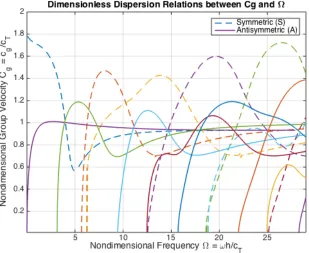
Figure 2.1 Theoretical curves on aluminum plate of thickness 4.72 mm for phase velocity cp and group velocity cg.
Group velocity relation can be represented by a closed form
ˆ
4
4 ˆk2ˆ
q2
1 pˆ ˆ q
tan( ˆp/ 2) tan( ˆq/ 2) (2.1.19) Or (2.1.20)
where G = 0 and pˆ/ 2 represent symmetric and anti-symmetric modes, respectively and the non-dimensional variables are defined by
, ˆ
h/cT kˆkh/
, ˆ
p2(ph/)2 2ˆ2kˆ2 qˆ2 (qh/)2 ˆ2kˆ2