symmetry
S S
Article
A Bidirectional Diagnosis Algorithm of Fuzzy Petri
Net Using Inner-Reasoning-Path
Kai-Qing Zhou1,2,*ID, Wei-Hua Gui1, Li-Ping Mo2and Azlan Mohd Zain3
1 College of Information Science and Engineering, Central South University, Changsha 410083, China;
2 College of Information Science and Engineering, Jishou University, Jishou 416000, China; [email protected]
3 Soft Computing Research Group, Faculty of computing, Universiti Teknologi Malaysia, Skudai 81310, Johor,
Malaysia; [email protected]
* Correspondence: [email protected]; Tel.: +86-0743-856-3673
Received: 1 May 2018; Accepted: 25 May 2018; Published: 1 June 2018
Abstract:Fuzzy Petri net (FPN) is a powerful tool to execute the fault diagnosis function for various industrial applications. One of the most popular approaches for fault diagnosis is to calculate the corresponding algebra forms which record flow information and three parameters of value of all places and transitions of the FPN model. However, with the rapid growth of the complexity of the real system, the scale of the corresponding FPN is also increased sharply. It indicates that the complexity of the fault diagnosis algorithm is also raised due to the increased scale of vectors and matrix. Focusing on this situation, a bidirectional adaptive fault diagnosis algorithm is presented in this article to reduce the complexity of the fault diagnosis process via removing irrelevant places and transitions of the large-scale FPN, followed by the correctness and algorithm complexity of the proposed approach that are also discussed in detail. A practical example is utilized to show the feasibility and efficacy of the proposed method. The results of the experiments illustrated that the proposed algorithm owns the ability to simplify the inference process and to reduce the algorithm complexity due to the removal of unnecessary places and transitions in the reasoning path of the appointed output place.
Keywords:fuzzy petri net; fault diagnosis; inner-reasoning-path; correctness; algorithm complexity
1. Introduction
With the increasing complexity of real systems, multifarious mechanisms have been presented to implement the inference process: expert system [1–4], Bayesian network [5], neural fuzzy system [6–11], multi-class diagnostic technique [12], Petri net (PN) [13,14], fuzzy Petri net (FPN) [15–17], etc. Among these techniques, FPN inherits the graphical nature and mathematical foundation of PN and represents the fuzzy production rule (FPR) accurately. Besides that, FPN can implement the dynamic inference process using different reasoning mechanisms. Owing to the advantages above, FPN has been applied in various fields to implement inference [18–23].
Ever since Looney (1998) proposed the forward fuzzy reasoning method using FPN for rule-based decision making [24], it has received much attention in the field of fault diagnosis to implement reasoning by FPN [25]. According to the existing literature, the main approach of fault diagnosis using FPN could be classified into two type: inference utilizing reachability tree-based analysis strategy and reasoning using the algebraic forms. Based on the former method, various reasoning algorithms based on fuzzy Petri net were proposed to implement knowledge representation and forward/backward inference [26–29]. The first strategy has some benefits as it can generate the reachability tree easily and analyze the reasoning process clearly. However, this approach still has some drawbacks such as
difficulty utilizing the parallel reasoning ability and modeling large-scale knowledge-based systems (KBS). Thus, to make the most of the parallel operational ability of FPN, the second method, namely reasoning mechanism using the algebraic forms, was proposed to analyze and implement the reasoning process. Gao et al. proposed a parallel reasoning algorithm using max-algebra, and they presented an improved reasoning algorithm based on the novel fuzzy reasoning Petri net (FRPN) to represent and reason the KBS with the negative literals [30,31]. In addition, there are other similar algorithms that have been proposed by other researchers [32–34]. Although fault diagnosis algorithms using FPN have been known to be successful, the existing algorithms are facing an enormous challenge called state explosion issue where the scale of FPN would increase with the rapid growth of the scale of KBS. The side-effect of the state explosion issue is to make the scale of related vectors and matrix of FPN using the second fault diagnosis mechanism by algebra forms increase sharply. It further indicates that the complexity and difficulty of the corresponding fault diagnosis algorithm is also increasing.
Focusing on the problematic issues, a bidirectional adaptive fault diagnosis algorithm by FPN is proposed to optimize and simplify the reasoning process based on our previous work, to generate an equivalent FPN model for the corresponding large-scale knowledge-based systems and to decompose the large scale FPN into a series of sub-FPNs surrounding the inner-inference-paths among fuzzy Petri nets [35,36]. The main thinking of the proposed algorithm is to reduce the complexity of fault diagnosis processing by removing the unnecessary places and transitions in the inference path of the appointed output place. To realize this presented function, the proposed algorithm has three phases: (1) using a backward reasoning mechanism to seek the unconcerned places and transitions; (2) implementing delete row or column commands to compress the dimension of the operational matrices; and (3) executing the forward reasoning strategy to calculate the truth degree of the goal on the simplified FPN. A practical example of turbine fault diagnosis system is employed to provide the feasibility and efficacy of the proposed method. The results of the experiments prove the proposed algorithm can select the optimum reasoning path of the appointed output place.
The rest of this article is organized as follows: Section2introduces the basis of FPN. Section3 presents the proposed algorithm in detail. Section4analyzes the correctness and complexity of the proposed algorithm. Section5illustrates the feasibly and validity of the proposed algorithm via a case study. Section6concludes this article.
2. Fuzzy Petri Net
In this section, the formality and relevant notions of FPN are discussed. Following that, the corresponding operators in the inference process are also generated.
2.1. Fuzzy Petri Net and Related Definitions
Focusing on the fault diagnosis issue, an FPN formalism is proposed in this article based on [37].
Definition 1.Fuzzy Petri Net.
The FPN is represented as an 8-tuple: FPN= (P,T,M,I,O,W,µ,CF), where
1. P={p1,p2,· · ·,pn}is a finite set of places. Moreover, X= (x1,x2,· · ·,xn)Tindicates a place vector, where|X|=|P|. If piis the goal place or a place which has a direct or indirect relationship with the goal place, xi =1. Else, xi =0.
2. T={t1,t2,· · ·,tm}is a finite set of transitions. Moreover, Y= (y1,y2,· · ·,ym)Tindicates a transit vector, where|Y|=|T|. If tjis the transition which has a direct or indirect relationship of the goal place, yj=1. Else, yj =0.
Symmetry2018,10, 192 3 of 15
I(pi,tj) = (
1 if there is an arc frompito tj
0 otherwise
4. O:T×P→(O(tj,pi))m×n is an output matrix. Here, O(tj,pi)n×mrecords whether a directed arc from tjto pi(j=1, 2,· · ·,m;i=1, 2,· · ·,n)exists, where
O(tj,pi) =
(
1 if there is an arc from tjtopi
0 otherwise
5. M = (m1,m2,· · ·,mn)T is a vector of fuzzy marking, where mi ∈ [0, 1]means the truth degree of corresponding place pi(i=1, 2,· · ·,n). The initial truth degree vector is denoted by M0.
6. µ:µ→(0, 1],µiis the threshold of tj. Moreover, D= (µ1,µ2,· · ·,µm)Tis a threshold vector, where
µj∈(0, 1] (j=1, 2,· · ·,m);
7. W(i,j)is the weight of the arc from pito tj. w(i,j)∈[0, 1]indicates how much the place piimpacts its following transition tj;
8. CF is the belief strength, where CFij ∈ (0, 1]indicates how much of a transition tjimpacts its output places pi.
Definition 2.Pre-set and Post-set.
For an FPN∑ = (P,T,M,W,µ,CF),•x ={y|(y,x)∈ F}is the pre-set or input set of x and x• = {y|(x,y)∈F}is the post-set or output set of x, where x,y∈P∪T. F is a flow relationship.
Definition 3.Input place and Output place.
If p={p∈P|•p=∅∧p•6=∅}, place p is an input place. If p={p∈P|•p6=∅∧p•=∅}, place p is an output place.
Definition 4.Enable and fired.
For a transition tj∈T, if there exists M(pi)·w(i,j)≥µ(tj), transition tjis enabled in the condition of marking M and denoted by M[tj. Moreover, if transition tjis enabled in the condition of making M, then a new marking M0could be obtained after tjfired and denoted by M[tj>M0.
Additional, an input strength vector I is defined as I= (I1,I2,· · ·,Ii)T(i=1, 2,· · ·,n)to records the input strength value of each place pi, where, Ii =M(pi)·w(i,j).
Definition 5.Incidence Matrix, Input Weight Matrix, and Output Belief Strength Matrix. Incidence matrix H is defined as H= (hij)n×m(i=1, 2,· · ·,n;j=1, 2,· · ·,m), where,
hij=
1 i f pi∈•tj −1 i f pi∈tj• 0 otherwise
Input Weight Matrix A is defined as A= (aij)n×m(i=1, 2,· · ·,n;j=1, 2,· · ·,m), where aij∈(0, 1] is the weight from pito tj. If pi ∈•tj, there are aij =wij. Else, aij =0.
2.2. Proposed Operators of the Proposed Algorithm
In the proposed algorithm, to delete the row or column in the operational matrices, the operators of these delete rows and columns are defined as follows.
Definition 6.Operators of Delete Rows and Columns.
Assume vector V is the vector to record the locations of rows which need to be deleted. Operator matrixname(V, :) = []; %is designed to delete the appointed rows.
Assume vector W is the vector to record the locations of columns which need to be deleted. Operator matrixname(:,W) = []; %is designed to delete the appointed columns.
Definition 7.Three operators of Max Algebra.
⊕:X⊕Y=Z,Zij=max(xij,yij),where, X,Y,Z are the n×m-dimensional matrices.
⊗ : X⊗Y = Z,Zij = max(xik,ykj)(k =, 1, 2,· · ·,s), where X,Y,Z are the n×s,s×m,n× m-dimensional matrices, respectively.
Θ:XΘY=Z. If xij ≥yij,zij=yij. Else, zij=0.
3. Bidirectional Adaptive Reasoning Algorithm
An acyclic net is a net which does not have a loop or circuit structure. According to reference [38,39], there does not exist circularity structure in the practically KBS. Based on this finding, the research focuses on how to implement the inference on the acyclic FPN. Thus, the proposed algorithm would only just consider the situation of the acyclic FPN model.
The related concepts of the proposed algorithm are listed as follows. (The assumption is that the FPN model has its ownnplaces andmtransitions in the reasoning process.)
3.1. The Proposed Algorithm
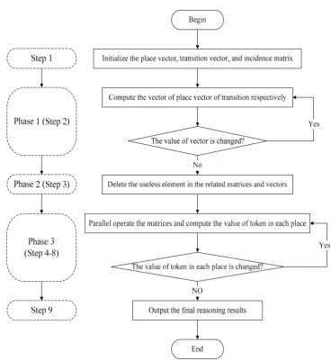
In the algorithm, to compress the scale of the operational matrices, a bidirectional reasoning algorithm is presented with combined highlights and a forward reasoning strategy with backward reasoning mechanism. The backward reasoning mechanism is employed to seek the unnecessary places and transitions to the forward reasoning strategy which is used to calculate the truth degree of the goal on the simplified FPN. The entire flowchart is drawn as shown in Figure1.
Symmetry2018,10, 192 5 of 15
Symmetry 2018, 10, x FOR PEER REVIEW 5 of 15
Figure 1. Flowchart of the Proposed Algorithm.
3.2. Implementation Steps
The implementation of the proposed algorithm could be separated into nine steps: Step 1: Initialize the place vector, transition vector, and incidence matrix.
In the initial place vector 0 ( , , , )1 2 T n
X = x x x , if place pi is the goal place, mark the
correspondence xi as 1. Else, xi is marked as 0. Moreover, each element of the initial transition
vector is marked as 0, where 0 (0,0, ,0) T
Y = .
Step 2: Assume i=1.
First, calculate ( ) 1
T
i i
Y = −H ⊗X− , 1
T
i i i
X =H ⊗ ⊕Y X− , and i+ + repeatedly until Yi =Yi−1 is
satisfied.
Then, execute X =X Y Yi, = i. (In vector X Y, , one represents the related places or transition of
the goal place.)
Step 3: Make V = all locations of elements whose value is 0 in X, and W = the location of elements whose value is 0 in Y . Then, using the proposed operators of delete rows and columns to update the input weighted matrix A', output belief strength matrix B', threshold vector D', and fuzzy marking vector M'.
Step 4: Assume k=0, Imax =(0 ,0 , ,0 )1 2 n . Then, execute I 1 ' ' T k+ =A M k.
Step 5: Execute I'k+1=IK+1ΘImax, and judge whether I'k+1 >Imax(previous). If it is true, it reveals that a
new transition can be enabled in the reasoning process. Then, execute Imax=Ik+1⊕Imax(previous). Else,
1
I'k+ =0 and move to Step 9.
Figure 1.Flowchart of the Proposed Algorithm.
3.2. Implementation Steps
The implementation of the proposed algorithm could be separated into nine steps: Step 1: Initialize the place vector, transition vector, and incidence matrix.
In the initial place vector X0 = (x1,x2,· · ·,xn)T, if place pi is the goal place, mark the correspondencexi as 1. Else, xi is marked as 0. Moreover, each element of the initial transition vector is marked as 0, whereY0= (0, 0,· · ·, 0)T.
Step 2: Assumei=1.
First, calculateYi = (−HT)⊗Xi−1,Xi = HT⊗Yi⊕Xi−1, andi+ +repeatedly untilYi =Yi−1 is satisfied.
Then, executeX=Xi,Y=Yi. (In vectorX,Y, one represents the related places or transition of the goal place.)
Step 3: MakeV =all locations of elements whose value is 0 in X, andW = the location of elements whose value is 0 inY. Then, using the proposed operators of delete rows and columns to update the input weighted matrixA0, output belief strength matrixB0, threshold vectorD0, and fuzzy marking vectorM0.
Step 5: Execute I0k+1= IK+1ΘImax, and judge whether I0k+1> Imax(previous). If it is true, it reveals that a new transition can be enabled in the reasoning process. Then, executeImax= Ik+1⊕Imax(previous). Else, I0k+1=0 and move to Step 9.
Step 6: ExecuteSk+1= ImaxΘD0, and judge whetherSk+1≥D. Then, Fire the related transition. Else, move to Step 9.
Step 7: ExecuteU0k+1 = B0⊗Sk+1, whereU0k+1represents the belief strength of output place with the fired transition in Step 6.
Step 8: ExecuteM0k+1 =U0k+1⊕M0kto get the latest update belief strength of all places. Then, judge whetherMk+0 1=Mk0. If it is true, move to Step 9. Else, move to Step 4.
Step 9: The whole reasoning process is stopped, and the final result is recorded inM0k+1.
4. Analysis
This section presents the theoretical analysis of the proposed algorithm from two different viewpoints: correctness and algorithm complexity.
4.1. Correctness
The analysis of correctness of the proposed algorithm is organized and based on two phases: backward reasoning phase and forward reasoning phase.
In the backward reasoning phase,xk=1(k=1, 2,· · ·,n)means thatpkis the goal in the initial place vector.
Wheni=1, performY1= (−HT)⊗X0,yj= max
1≤k≤n(−hij×xk)(j=1, 2,· · ·,m). Ifhij=−1 and xk =1, thenyj =1 can be obtained (yj =1 meanspk∈ tj•). Then,Y1= (−HT)⊗X0is used to add the input transitiontjof goal placepkinto the transition vectorY.
InX1 = H⊗Y1⊕X0,H⊗Y1is analyzed first. AssumeZ = H⊗Y1, where Zs = max 1≤k≤n(hij× bj)(s=1, 2,· · ·,m). Ifhij=1 andyj =1, thenZs =1 can be obtained whereZs=1 meanspk∈•tj. Hence, the function ofZ= H⊗Yis to add the input place of input transitiontjof conclusion placepk into the vectorZ. Furthermore,X1= H⊗Y1⊕X0 =Z⊕X0reflects the set of related places of the goal placepk.
In the repeated part of Figure1, with the increasing ofi(i = 1, 2,· · ·,n), the equationsYi = (−HT)⊗Xi−1andXi = H⊗Yi⊕Xi−1, can also be easily understood based on the thinking of the situationi=1.
Based on the analysis above, the correctness of backward reasoning phase has been proven. In comparison to the backward reasoning phase, the forward reasoning phase uses four equations to implement the reasoning process.
When k = 0, I1 = A0TM00. iz = n
∑
j=1
wzj·mjz(z = 1, 2,· · ·,m)is the input strength of each
transition. Then, I0k+1 =IK+1ΘImax.i0z =
(
iz iz≥izmax
0 else (z=1, 2,· · ·,m)is used to judge whether a new transition exists in the reasoning path. In addition, if there is a new transition, the equation Imax= IK+1⊕Imax(previous)will be used to update the newest data.
Sk+1 = ImaxΘD0. Sz = (
izmax izmax≥µ
0 else is used to judge which transitions can be enabled. After firing the transition, M0k+1 = B⊗Sk+1is used to record the belief strength of output place related to the fired transition. To sum up, these equations in the forward reasoning phase are used to judge the transition that can be fired and implement the reasoning process step by step.
Symmetry2018,10, 192 7 of 15
4.2. Algorithm Complexity
The algorithm complexity is presented in two phases.
In the backward reasoning phase, the algorithm is used to analyze the worst situation where only one transition is added into the transition vectorYeach time. In the(m+1)th repeat, no transition can be added intoY.Yi+1=Yexists at this time. Thus, the biggest circle number ism+1. Accordingly, the matrix can implement parallel analysis and computation and the algorithm complexity of backward reasoning phase isO(n×m).
After implementing the backward reasoning mechanism, the dimensions of the operational matrices are reduced to(n−r)×(m−p)fromn×m, wherer,pare the number of irrelevant places or transitions.
In the forward reasoning phase, the algorithm complexity is related to the dimension of operational matrices. Thus, the algorithm complexity of forward reasoning algorithm isO((n− r)×(m−p)).
To conclude this section, the proposed algorithm is summarized into two situations as follows.
1. In the worst situation, all places and transitions appear in the reasoning path. This means that the backward reasoning mechanism is out of work. The algorithm complexity of the proposed algorithm isO(n×m).
2. In other situations, the number of unconcerned places and transitions are r and p, and the algorithm complexity of the proposed algorithm isO((n−r)×(m−p)).
5. Case Study
In this section, a numerical case study is reported to demonstrate the whole reasoning process of the present reasoning algorithm, particularly the potential of the proposed method for simplifying the inference process and reducing the algorithm complexity based different appointed output places.
In the experiment, the FPN models adopted in this study should meet three requirements to reflect the algorithm feasibility. First, three types of FPN models are included in the model. Second, the model should contain two or more of the final conclusions (i.e., output places). Third, other special cases, such as a certain place where a pre-set is greater than or equal to two transitions or a subsequent place that is greater than or equal to two transitions, is considered. This study accordingly uses the fault diagnosis case for an integrated manufacturing system in the literature [26] to demonstrate the proposed decomposition of the algorithm.
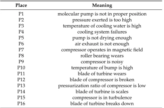
The corresponding FPN model is generated as shown in Figure2and the meaning of each place is listed in Table1.
Table 1.The meaning of each place of Figure2.
Place Meaning
P1 molecular pump is not in proper position
P2 pressure exerted is too high
P3 temperature of cooling water is high
P4 cooling system failures
P5 pump is not drying enough
P6 air exhaust is not enough
P7 compressor operates in magnetic field
P8 roller bearing wears
P9 compressor is noisy
P10 temperature of bump is high
P11 blade of turbine wears
P12 blade of compressor is broken
P13 pressurization ratio of compressor is low
P14 blade of turbine is scales
P15 compressor is in turbulence
Symmetry 2018, 10, x FOR PEER REVIEW 8 of 15
Figure 2. The Fuzzy Petri net (FPN) of case study.
5.1. Relevant Experimental Data of the Case Study
Assume the initial marking vector is defined as follows.
0 (0.85,0.7,0.75,0.8,0,0,0,0,0,0,0,0,0,0,0,0)
T
M =
The H H A,− T,
and B of the case study are illustrated as follows.
− − − − − − − − − − − − − = 1 0 0 0 0 0 0 0 0 0 0 0 1 0 0 0 0 0 0 0 0 0 1 0 1 0 0 0 0 0 0 0 0 0 1 1 0 0 0 0 0 0 0 0 0 1 0 1 1 0 0 0 0 0 0 0 0 1 0 0 1 0 0 0 0 0 0 0 0 1 0 1 1 0 0 0 0 0 0 0 0 1 0 0 1 0 0 0 0 0 0 0 0 1 0 0 1 0 0 0 0 0 0 0 0 1 0 0 1 0 0 0 0 0 0 0 0 1 0 0 1 0 0 0 0 0 0 0 1 0 0 0 0 0 0 0 0 0 0 0 1 0 0 0 0 0 0 0 0 0 0 1 0 0 0 0 0 0 0 0 0 0 1 1 0 0 0 0 0 0 0 0 0 0 0 1 H = − 1 0 1 -0 0 0 0 0 0 0 0 0 0 0 0 0 0 1 0 1 -1 -0 0 0 0 0 0 0 0 0 0 0 0 0 1 1 0 1 -0 0 0 0 0 0 0 0 0 0 0 0 0 0 1 0 1 -0 0 0 0 0 0 0 0 0 0 0 0 0 1 0 0 1 -0 0 0 0 0 0 0 0 0 0 0 0 0 1 1 0 1 -0 0 0 0 0 0 0 0 0 0 0 0 0 1 0 0 1 -0 0 0 0 0 0 0 0 0 0 0 0 0 1 0 0 1 -1 -0 0 0 0 0 0 0 0 0 0 0 0 1 0 0 0 1 -1 -1 -0 0 0 0 0 0 0 0 0 0 1 0 0 0 0 1 -0 0 0 0 0 0 0 0 0 0 0 1 0 0 0 0 1 -T H
Figure 2.The Fuzzy Petri net (FPN) of case study.
5.1. Relevant Experimental Data of the Case Study
Assume the initial marking vector is defined as follows.
M0= (0.85, 0.7, 0.75, 0.8, 0, 0, 0, 0, 0, 0, 0, 0, 0, 0, 0, 0)T
TheH,−HT,AandBof the case study are illustrated as follows.
H=
1 0 0 0 0 0 0 0 0 0 0
0 1 1 0 0 0 0 0 0 0 0
0 0 1 0 0 0 0 0 0 0 0
0 0 1 0 0 0 0 0 0 0 0
0 0 0 1 0 0 0 0 0 0 0
−1 0 0 1 0 0 0 0 0 0 0
0 −1 0 0 1 0 0 0 0 0 0
0 0 −1 0 0 1 0 0 0 0 0
0 0 0 −1 0 0 1 0 0 0 0
0 0 0 0 −1 −1 0 1 0 0 0
0 0 0 0 0 −1 0 0 1 0 0
0 0 0 0 0 0 −1 −1 0 1 0
0 0 0 0 0 0 0 0 −1 1 0
0 0 0 0 0 0 0 0 −1 0 1
0 0 0 0 0 0 0 0 0 −1 0
0 0 0 0 0 0 0 0 0 0 −1
−HT=
−1 0 0 0 0 1 0 0 0 0 0 0 0 0 0 0
0 −1 0 0 0 0 1 0 0 0 0 0 0 0 0 0
0 −1 −1 −1 0 0 0 1 0 0 0 0 0 0 0 0
0 0 0 0 −1 −1 0 0 1 0 0 0 0 0 0 0
0 0 0 0 0 0 −1 0 0 1 0 0 0 0 0 0
0 0 0 0 0 0 0 −1 0 1 1 0 0 0 0 0
0 0 0 0 0 0 0 0 −1 0 0 1 0 0 0 0
0 0 0 0 0 0 0 0 0 −1 0 1 0 0 0 0
0 0 0 0 0 0 0 0 0 0 −1 0 1 1 0 0
0 0 0 0 0 0 0 0 0 0 0 −1 −1 0 1 0
0 0 0 0 0 0 0 0 0 0 0 0 0 −1 0 1
Symmetry2018,10, 192 9 of 15
A=
1 0 0 0 0 0 0 0 0 0 0
0 1 0.3 0 0 0 0 0 0 0 0 0 0 0.5 0 0 0 0 0 0 0 0 0 0 0.2 0 0 0 0 0 0 0 0 0 0 0 0.5 0 0 0 0 0 0 0 0 0 0 0.5 0 0 0 0 0 0 0
0 0 0 0 1 0 0 0 0 0 0
0 0 0 0 0 1 0 0 0 0 0
0 0 0 0 0 0 1 0 0 0 0
0 0 0 0 0 0 0 1 0 0 0
0 0 0 0 0 0 0 0 1 0 0
0 0 0 0 0 0 0 0 0 0.7 0 0 0 0 0 0 0 0 0 0 0.3 0
0 0 0 0 0 0 0 0 0 0 1
0 0 0 0 0 0 0 0 0 0 0
0 0 0 0 0 0 0 0 0 0 0
B=
0 0 0 0 0 0 0 0 0 0 0
0 0 0 0 0 0 0 0 0 0 0
0 0 0 0 0 0 0 0 0 0 0
0 0 0 0 0 0 0 0 0 0 0
0 0 0 0 0 0 0 0 0 0 0
0.9 0 0 0 0 0 0 0 0 0 0
0 0.8 0 0 0 0 0 0 0 0 0
0 0 0.9 0 0 0 0 0 0 0 0
0 0 0 0.8 0 0 0 0 0 0 0
0 0 0 0 0.95 0.9 0 0 0 0 0
0 0 0 0 0 0.7 0 0 0 0 0
0 0 0 0 0 0 0.9 0.95 0 0 0
0 0 0 0 0 0 0 0 0.9 0 0
0 0 0 0 0 0 0 0 0.8 0 0
0 0 0 0 0 0 0 0 0 0.95 0
0 0 0 0 0 0 0 0 0 0 0.8
5.2. Experiments
According to the case study, two experiments are designed based on different appointed goal output place. In Experiment 1, the goal output place isp15. In Experiment 2, the goal output place is changed top16.
5.2.1. Experiment One
Experiment 1 aims at trying to get the truth degree ofp15in Figure2.
The initial place vectorXand transition vectorYare demonstrated as follows.
initial X= (0, 0, 0, 0, 0, 0, 0, 0, 0, 0, 0, 0, 0, 0, 1, 0)T initial Y= (0, 0, 0, 0, 0, 0, 0, 0, 0, 0, 0)T
After performing the backward reasoning phase, the relevant vectors and matrices are gained as follows.
X0 = (1, 1, 1, 1, 1, 1, 1, 1, 1, 1, 1, 1, 1, 0, 1, 0)T Y0= (1, 1, 1, 1, 1, 1, 1, 1, 1, 1, 0)T
Symmetry 2018, 10, x FOR PEER REVIEW 10 of 15 0.4 P1 P2 P3 P6 P7 P8 P5 P9 P10 P11 P12 P13 P15 t3 t2 t1 1 1 0.5 t4 t5 t6 t7 t8 t9 t10 0.9 0.5 0.8 1
0.95 0.9 1 0.9 0.8 1 1 0.7 0.95 1 0.3 0.3 0.2 0.3 0.1 0.2 0.3 0.2 0.2
Figure 3. The reasoning path of goal place p15.
After executing Phases 1 and 2 of the proposed algorithm, the subnet of the goal output place is obtained as shown in Figure 3. The related data (including vectors and matrices) are also modified based on the result of previous phases. The simplified data are given below.
0
' (0.85,0.7,0.75,0.8,0,0,0,0,0,0,0,0,0,0)T
M = '0 (0.3,0.2,0.3,0.3,0.1,0.2,0.3,0.2,0.2,0.2) T
D =
1 0 0 0 0 0 0 0 0 0 0 1 0 .3 0 0 0 0 0 0 0 0 0 0 .5 0 0 0 0 0 0 0 0 0 0 .2 0 0 0 0 0 0 0 0 0 0 0 .5 0 0 0 0 0 0 0 0 0 0 .5 0 0 0 0 0 0 0 0 0 0 1 0 0 0 0 0 '
0 0 0 0 0 1 0 0 0 0 0 0 0 0 0 0 1 0 0 0 0 0 0 0 0 0 0 1 0 0 0 0 0 0 0 0 0 0 1 0 0 0 0 0 0 0 0 0 0 0 .7 0 0 0 0 0 0 0 0 0 0 .3 0 0 0 0 0 0 0 0 0 0
A =
0 0 0 0 0 0 0 0 0 0
0 0 0 0 0 0 0 0 0 0
0 0 0 0 0 0 0 0 0 0
0 0 0 0 0 0 0 0 0 0
0 0 0 0 0 0 0 0 0 0
0 .9 0 0 0 0 0 0 0 0 0
0 0 .8 0 0 0 0 0 0 0 0
'
0 0 0 .9 0 0 0 0 0 0 0
0 0 0 0 .8 0 0 0 0 0 0
0 0 0 0 0 .9 0 .9 0 0 0 0
0 0 0 0 0 0 .7 0 0 0 0
0 0 0 0 0 0 0 .9 0 .9 0 0
0 0 0 0 0 0 0 0 0 .9 0
0 0 0 0 0 0 0 0 0 0 .9
B =
1.0 0 0 0 0 0 0 0 0 0 0 0 0 1.0 0 0 0 0 0 0 0 0 0 0 0 0 0 0.3 0.5 0.2 0 0 0 0 0 0 0 0 0 0 0 0 0 0 0.5 0.5 0 0 0 0 0 0 0 0 0 0 0 0 0 0 1.0 0 0 0 0 0 0 0 '
0 0 0 0 0 0 0 1.0 0 0 0 0 0 0 0 0 0 0 0 0 0 0 1.0 0 0 0 0 0 0 0 0 0 0 0 0 0 0 1.0 0 0 0 0 0 0 0 0 0 0 0 0 0 0 1.0 0 0 0 0 0 0 0 0 0 0 0 0 0 0 0.7 0.3 0
T A =
Based on the modified data, the details of performing the forward reasoning strategy are demonstrated, as shown in Tables 2 and 3, respectively.
According to Table 3, it is easy to get that the final truth degree of p15 is 0.582415 after repeating
the inference process five times.
Figure 3.The reasoning path of goal placep15.
After executing Phases 1 and 2 of the proposed algorithm, the subnet of the goal output place is obtained as shown in Figure3. The related data (including vectors and matrices) are also modified based on the result of previous phases. The simplified data are given below.
M00= (0.85, 0.7, 0.75, 0.8, 0, 0, 0, 0, 0, 0, 0, 0, 0, 0)T D00= (0.3, 0.2, 0.3, 0.3, 0.1, 0.2, 0.3, 0.2, 0.2, 0.2)T
A0=
1 0 0 0 0 0 0 0 0 0
0 1 0.3 0 0 0 0 0 0 0
0 0 0.5 0 0 0 0 0 0 0
0 0 0.2 0 0 0 0 0 0 0
0 0 0 0.5 0 0 0 0 0 0
0 0 0 0.5 0 0 0 0 0 0
0 0 0 0 1 0 0 0 0 0
0 0 0 0 0 1 0 0 0 0
0 0 0 0 0 0 1 0 0 0
0 0 0 0 0 0 0 1 0 0
0 0 0 0 0 0 0 0 1 0
0 0 0 0 0 0 0 0 0 0.7
0 0 0 0 0 0 0 0 0 0.3
0 0 0 0 0 0 0 0 0 0
B0=
0 0 0 0 0 0 0 0 0 0
0 0 0 0 0 0 0 0 0 0
0 0 0 0 0 0 0 0 0 0
0 0 0 0 0 0 0 0 0 0
0 0 0 0 0 0 0 0 0 0
0.9 0 0 0 0 0 0 0 0 0
0 0.8 0 0 0 0 0 0 0 0
0 0 0.9 0 0 0 0 0 0 0
0 0 0 0.8 0 0 0 0 0 0
0 0 0 0 0.9 0.9 0 0 0 0
0 0 0 0 0 0.7 0 0 0 0
0 0 0 0 0 0 0.9 0.9 0 0
0 0 0 0 0 0 0 0 0.9 0
0 0 0 0 0 0 0 0 0 0.9
A0T=
1.0 0 0 0 0 0 0 0 0 0 0 0
0 1.0 0 0 0 0 0 0 0 0 0 0 0 0
0 0.3 0.5 0.2 0 0 0 0 0 0 0 0 0 0
0 0 0 0 0.5 0.5 0 0 0 0 0 0 0 0
0 0 0 0 0 0 1.0 0 0 0 0 0 0 0
0 0 0 0 0 0 0 1.0 0 0 0 0 0 0
0 0 0 0 0 0 0 0 1.0 0 0 0 0 0
0 0 0 0 0 0 0 0 0 1.0 0 0 0 0
0 0 0 0 0 0 0 0 0 0 1.0 0 0 0
0 0 0 0 0 0 0 0 0 0 0 0.7 0.3 0
Based on the modified data, the details of performing the forward reasoning strategy are demonstrated, as shown in Tables2and3, respectively.
Symmetry2018,10, 192 11 of 15
Table 2.The recovery procedure of output strength vector of Experiment 1.
Repeat Output Strength Vector
1st (0.85, 0.9, 0.865, 0, 0, 0, 0, 0, 0, 0)T
2nd (0.85, 0.9, 0.865, 0.3825, 0.72, 0.7785, 0, 0, 0, 0)T
3rd (0.85, 0.9, 0.865, 0.3825, 0.72, 0.7785, 0.306, 0.70065, 054495, 0)T
4th (0.85, 0.9, 0.865, 0.3825, 0.72, 0.7785, 0.306, 0.70065, 054495, 0.613069)T
5th (0.85, 0.9, 0.865, 0.3825, 0.72, 0.7785, 0.306, 0.70065, 054495, 0.613069)T
Table 3.The forward reasoning process of Experiment 1.
Repeat M0
1st (0.85, 0.9, 0.85, 0.85, 0, 0.765, 0.72, 0.7785, 0, 0, 0, 0, 0, 0)T
2nd (0.85, 0.9, 0.85, 0.85, 0, 0.765, 0.72, 0.7785, 0.306, 070065, 054495, 0, 0, 0)T
3rd (0.85, 0.9, 0.85, 0.85, 0, 0.765, 0.72, 0.7785, 0.306, 0.70065, 0.54495, 0.665618, 0.490455, 0)T
4th (0.85, 0.9, 0.85, 0.85, 0, 0.765, 0.72, 0.7785, 0.306, 0.70065, 0.54495, 0.665618, 0.490455, 0.582415)T
5th (0.85, 0.9, 0.85, 0.85, 0, 0.765, 0.72, 0.7785, 0.306, 0.70065, 0.54495, 0.665618, 0.490455, 0.582415)T
5.2.2. Experiment Two
Experiment 2 is meant to try to calculate the truth degree of another output placep16by using the same FPN model shown in Figure2.
The initial place vectorX, transition vectorYare demonstrated as follows.
initial X= (0, 0, 0, 0, 0, 0, 0, 0, 0, 0, 0, 0, 0, 0, 0, 1)T initial Y= (0, 0, 0, 0, 0, 0, 0, 0, 0, 0, 0)T
After performing the backward reasoning phase, the relevant vectors and matrices are gained as follows.
X0 = (0, 1, 1, 1, 0, 0, 0, 1, 0, 0, 1, 0, 0, 1, 0, 1)T Y0= (0, 0, 1, 0, 0, 1, 0, 0, 1, 0, 1)T
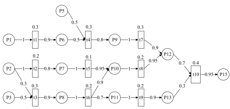
According to theX0,Y0, the reasoning path of goal placep16is demonstrated as shown in Figure4 after deleting the irrelevant element in FPN.
Symmetry 2018, 10, x FOR PEER REVIEW 11 of 15
Table 2. The recovery procedure of output strength vector of Experiment 1.
Repeat Output Strength Vector
1st (0.85,0.9,0.865,0,0,0,0,0,0,0)T
2nd (0.85,0.9,0.865,0.3825,0.72,0.7785,0,0,0,0)T
3rd (0.85,0.9,0.865,0.3825,0.72,0.7785,0.306,0.70065,054495,0)T
4th (0.85,0.9,0.865,0.3825,0.72,0.7785,0.306,0.70065,054495,0.613069)T
5th (0.85,0.9,0.865,0.3825,0.72,0.7785,0.306,0.70065,054495,0.613069)T
Table 3. The forward reasoning process of Experiment 1.
Repeat M’
1st (0.85,0.9,0.85,0.85,0,0.765,0.72,0.7785,0,0,0,0,0,0)T
2nd (0.85,0.9,0.85,0.85,0,0.765,0.72,0.7785,0.306,070065,054495,0,0,0)T
3rd (0.85,0.9,0.85,0.85,0,0.765,0.72,0.7785,0.306,0.70065,0.54495,0.665618,0.490455,0)T
4th (0.85,0.9,0.85,0.85,0,0.765,0.72,0.7785,0.306,0.70065,0.54495,0.665618,0.490455,0.582415)T
5th (0.85,0.9,0.85,0.85,0,0.765,0.72,0.7785,0.306,0.70065,0.54495,0.665618,0.490455,0.582415)T
5.2.2. Experiment Two
Experiment 2 is meant to try to calculate the truth degree of another output place p16 by using
the same FPN model shown in Figure 2.
The initial place vector X, transition vector Y are demonstrated as follows.
(0,0,0,0,0,0,0,0,0,0,0,0,0,0,0,1)T (0,0,0,0,0,0,0,0,0,0,0)T
initial X = initial Y=
After performing the backward reasoning phase, the relevant vectors and matrices are gained as follows.
' (0,1,1,1,0,0,0,1,0,0,1,0,0,1,0,1)T ' (0,0,1,0,0,1,0,0,1,0,1)T
X = Y =
According to the X Y', ', the reasoning path of goal place p16 is demonstrated as shown in
Figure 4 after deleting the irrelevant element in FPN.
Figure 4. The reasoning path of goal place p16.
After executing Phases 1 and 2 of the proposed algorithm, the subnet of the goal output place is obtained as shown in Figure 4. The related data (including vectors and matrices) are also modified based on the result of previous phases. The simplified data are given below.
0
' (0.7,0.75,0.8,0,0,0,0,0)T
M = D'0 =(0.3,0.2,0.2,0.3)T Figure 4.The reasoning path of goal placep16.
After executing Phases 1 and 2 of the proposed algorithm, the subnet of the goal output place is obtained as shown in Figure4. The related data (including vectors and matrices) are also modified based on the result of previous phases. The simplified data are given below.
A0 =
0.3 0 0 0 0.5 0 0 0 0.2 0 0 0
0 1 0 0
0 0 1 0
0 0 0 1
0 0 0 0
B0=
0 0 0 0
0 0 0 0
0 0 0 0
0.9 0 0 0
0 0.7 0 0
0 0 0.8 0
0 0 0 0.8
A0T=
0.3 0.5 0.2 0 0 0 0
0 0 0 1 0 0 0
0 0 0 0 1 0 0
0 0 0 0 0 1 0
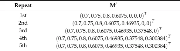
Based on the modified data, the details of the forward reasoning are demonstrated, as shown in Tables4and5, respectively.
Table 4.The recovery procedure of output strength vector of Experiment 2.
Repeat Output Strength Vector
1st (0.745, 0, 0, 0)T
2nd (0.745, 0.6705, 0, 0)T
3rd (0.745, 0.6705, 0.46935, 0)T
4th (0.745, 0.6705, 0.46935, 0.37548)T
5th (0.745, 0.6705, 0.46935, 0.37548)T
Table 5.The forward reasoning process of Experiment 2.
Repeat M0
1st (0.7, 0.75, 0.8, 0.6075, 0, 0, 0)T
2nd (0.7, 0.75, 0.8, 0.6075, 0.46935, 0, 0)T
3rd (0.7, 0.75, 0.8, 0.6075, 0.46935, 0.37548, 0)T
4th (0.7, 0.75, 0.8, 0.6075, 0.46935, 0.37548, 0.300384)T
5th (0.7, 0.75, 0.8, 0.6075, 0.46935, 0.37548, 0.300384)T
According to Table5, it is easy to get that the final truth degree ofp16is 0.300384 after repeating the inference process five times.
5.3. Analysis of Experiments 1 and 2
The two experiments used the same FPN model to calculate the truth degree of different output places. Although these inferences are implemented under the same framework, the details of the inference are different. Table6illustrates the comparison of the two experiments from the viewpoint of the related operational matrices.
Table 6.Comparison of Experiments.
Related Matrices Experiment One Experiment Two
Original Matrices H,AandB 16×11 16×11
−HT 11×16 11×16
In backward reasoning phase A
0andB0 16×11 16×11
A0T 11×16 11×16
In forward reasoning phase A
0andB0 14×10 7×4
Symmetry2018,10, 192 13 of 15
In Table6, it easily found that the scale of the operational matrices is compressed. In the case of Experiment 2, the scale of the original matricesAandBare 16×11 and−HT is 11×16. In the backward reasoning phase, these matrices are unitized to seek the reasoning path for the goal place. Then, irrelevant places and transitions are deleted by implementing operators. Finally, the dimensions of related matrices are reduced from 14×10 and 10×14 to 7×4 and 4×6, because the forward reasoning phase is executed in the individual reasoning path as shown in Figure4.
In the existing literature, the fault diagnosis mechanism using FPN algebra is that all elements (including places and transitions) of the FPN model are used to execute the fault diagnosis. However, with the rapidly increasing scale of FPN, the number of unrelated places and transitions of the goal outplace in a large-scale FPN is also increased. Hence, the biggest feature of the proposed algorithm is that the complexity of inference is adjusted by different goal places because of the removal of unnecessary places and transitions of the goal output places. The case study is a typical instance to indicate this advantage. Although these two experiments are implemented on the same FPN, the scales of related matrices are compressed from 16×11 and 11×16 to 7×4 and 4×7 based on the different reasoning paths.
In summary, the proposed mechanism will adjust the dimension of the related operational matrices and vectors in the reasoning process automatically because the individual reasoning path will be recognized based on different goal places. By implementing the fault diagnosis using large-scale FPNs, the inference process is more flexible and closer to human thinking
6. Conclusions
Focusing on the side-effect of state explosion issue of FPN, a bidirectional adaptive fault diagnosis algorithm has been presented in this paper to control the dimensions of the operational matrices and simplify the reasoning process by removing the irrelated elements (i.e., places and transitions) in a large-scale FPN model. In the proposed algorithm, the algorithm was implemented in three phases. Firstly, backward reasoning mechanism was executed to find the unconcerned places and transitions. Secondly, the delete row and column commands were used to compress the dimensional of the corresponding operational matrices. Finally, forward reasoning was implemented to calculate the truth degree of the goal place. After undergoing the three phases, a theoretical analysis was carried out to prove the feasibly and validity of the proposed algorithm from two aspects: correctness and algorithm complexity. Using the analysis, a case study of fault diagnosis was used to illustrate the whole implementation process. From the results of two experiments, it is easy to find that the proposed algorithm can overcome the state explosion issue effectively because the places and transitions that are not involved in the reasoning path will be removed automatically.
Author Contributions:K.-Q.Z. conceived and designed the experiments; W.-H.G. performed the experiments; L.-P.M. analyzed the data; K.-Q.Z. and A.M.Z. wrote the paper.
Acknowledgments:This work is supported by the National Natural Science Foundation of China (Nos. 61741205, 61462029 and 61363073), the Research Foundation of Education Bureau of Hunan Province, China (No. 16C1314) and Post-doctoral Science Foundation of Central South University (No. 175605).
Conflicts of Interest:The authors declare no conflict of interest.
References
1. Burrell, P.; Inman, D. An expert system for the analysis of faults in an electricity supply network: Problems and achievements.Comput. Ind.1998,37, 113–123. [CrossRef]
2. Liu, S.C.; Liu, S.Y. An efficient expert system for machine fault diagnosis.Int. J. Adv. Manuf. Technol.2003, 21, 691–698. [CrossRef]
3. Liu, H.; Gegov, A.; Cocea, M. Rule-based systems: A granular computing perspective.Granul. Comput.2016, 1, 259–274. [CrossRef]
5. Huang, Y.; McMurran, R.; Dhadyalla, G.; Jones, R.P. Probability based vehicle fault diagnosis: Bayesian network method.J. Intell. Manuf.2008,19, 301–311. [CrossRef]
6. Alessandri, A. Fault diagnosis for nonlinear systems using a bank of neural estimators.Comput. Ind.2003, 52, 271–289. [CrossRef]
7. Chen, K.Y.; Lim, C.P.; Lai, W.K. Application of a neural fuzzy system with rule extraction to fault detection and diagnosis.J. Intell. Manuf.2005,16, 679–691. [CrossRef]
8. Lai, Y.F.; Chen, M.Y.; Chiang, H.S. Constructing the lie detection system with fuzzy reasoning approach. Granul. Comput.2017,3, 169–176. [CrossRef]
9. Lukovac, V.; Pamuˇcar, D.; Popovi´c, M.;Đorovi´c, B. Portfolio model for analyzing human resources: An approach based on neuro-fuzzy modeling and the simulated annealing algorithm.Expert Syst. Appl.2017, 90, 318–331. [CrossRef]
10. Pamuˇcar, D.; Ljubojevi´c, S.; Kostadinovi´c, D.;Đorovi´c, B. Cost and risk aggregation in multi-objective route planning for hazardous materials transportation—A neuro-fuzzy and artificial bee colony approach. Expert Syst. Appl.2016,65, 1–15. [CrossRef]
11. Pamuˇcar, D.; Vasin, L.; Atanaskovi´c, P.; Miliˇci´c, M. Planning the City Logistics Terminal Location by Applying the Green-Median Model and Type-2 Neurofuzzy Network.Comput. Intell. Neurosci.2016,2016, 6972818. 12. Mortada, M.A.; Yacout, S.; Lakis, A. Fault diagnosis in power transformers using multi-class logical analysis
of data.J. Intell. Manuf.2013,25, 1429–1439. [CrossRef]
13. Reyes, A.; Yu, H.; Kelleher, G.; Lloyd, S. Integrating Petri Nets and hybrid heuristic search for the scheduling of FMS.Comput. Ind.2002,47, 123–138. [CrossRef]
14. Cecil, J.A.; Srihari, K.; Emerson, C.R. A review of Petri-net applications in manufacturing. Int. J. Adv. Manuf. Technol.1992,7, 168–177. [CrossRef]
15. Luo, X.; Kezunovic, M. Implementing fuzzy Reasoning Petri-Nets for fault section estimation.IEEE Trans. Power Deliv.2008,23, 676–685. [CrossRef]
16. Hu, H.; Li, Z.; Al-Ahmari, A. Reversed fuzzy Petri nets and their application for fault diagnosis. Comput. Ind. Eng.2011,60, 505–510. [CrossRef]
17. Yang, B.; Li, H. A novel dynamic timed fuzzy Petri nets modeling method with applications to industrial processes.Expert Syst. Appl.2018,97, 276–289. [CrossRef]
18. Pan, H.L.; Jiang, W.R.; He, H.H. The Fault Diagnosis Model of Flexible Manufacturing System Workflow Based on Adaptive Weighted Fuzzy Petri Net.Adv. Sci. Lett.2012,11, 811–814. [CrossRef]
19. Amin, M.; Shebl, D. Reasoning dynamic fuzzy systems based on adaptive fuzzy higher order Petri nets. Inf. Sci.2014,286, 161–172. [CrossRef]
20. Liang, W.; An, R. Unobservable fuzzy petri net diagnosis technique.Aircr. Eng. Aerosp. Technol.2013,85, 215–221.
21. Liu, H.C.; Lin QL Ren, M.L. Fault diagnosis and cause analysis using fuzzy evidential reasoning approach and dynamic adaptive fuzzy Petri nets.Comput. Ind. Eng.2013,66, 899–908. [CrossRef]
22. Wang, W.M.; Peng, X.; Zhu, G.N.; Hu, J.; Peng, Y.H. Dynamic representation of fuzzy knowledge based on fuzzy petri net and genetic-particle swarm optimization.Expert Syst. Appl.2014,41, 1369–1376. [CrossRef] 23. Liu, H.C.; You, J.X.; Tian, G. Determining Truth Degrees of Input Places in Fuzzy Petri Nets.IEEE Trans. Syst.
Man Cyber. Syst.2017,47, 3425–3431. [CrossRef]
24. Looney, C. G Fuzzy Petri nets for rule-based decision making.IEEE Trans. Syst. Man Cyber.1988,18, 178–183. [CrossRef]
25. Zhou, K.Q.; Zain, A.M. Fuzzy Petri Nets and Industrial Applications: A Review.Artif. Intell. Rev.2016,45, 405–446. [CrossRef]
26. Chen, S.M. Weighted fuzzy reasoning using Weighted Fuzzy Petri Nets.IEEE Trans. Knowl. Data Eng.2002, 14, 386–397. [CrossRef]
27. Liu, Z.; Li, H.; Zhou, P. Towards timed fuzzy Petri net algorithms for chemical abnormality monitoring. Expert Syst. Appl.2011,38, 9724–9728. [CrossRef]
28. Wai, R.J.; Liu, C.M. Design of dynamic petri recurrent fuzzy neural network and its application to path-tracking control of nonholonomic mobile robot.IEEE Trans. Ind. Electron.2009,56, 2667–2683. 29. Chen, S.M.; Ke, J.S.; Chang, J.F. Knowledge representation using fuzzy Petri nets. IEEE Trans. Knowl.
Symmetry2018,10, 192 15 of 15
30. Gao, M.M.; Wu, Z.M.; Zhou, M.C. A Petri net-based formal reasoning algorithm for fuzzy production rule-based systems.IEEE Int. Conf. Syst. Man Cyber.2000,4, 3093–3097.
31. Gao, M.M.; Zhou, M.C.; Huang, X.G.; Wu, Z.M. Fuzzy reasoning Petri nets.IEEE Trans. Syst. Man Cyber. Part A Syst. Hum.2003,33, 314–324.
32. Liu, H.C.; Luan, X.; Li, Z.; Wu, J. Linguistic Petri Nets Based on Cloud Model Theory for Knowledge Representation and Reasoning.IEEE Trans. Knowl. Data Eng.2018,30, 717–728. [CrossRef]
33. Guo, Y.; Meng, X.; Wang, D.; Meng, T.; Liu, S.; He, R. Comprehensive risk evaluation of long-distance oil and gas transportation pipelines using a fuzzy petri net model.J. Nat. Gas Sci. Eng.2016,33, 18–29. [CrossRef] 34. Li, H.; You, J.X.; Liu, H.C.; Tian, G. Acquiring and Sharing Tacit Knowledge Based on Interval 2-Tuple
Linguistic Assessments and Extended Fuzzy Petri Nets.Int. J. Uncertain. Fuzziness Knowl.-Based Syst.2018, 26, 43–65. [CrossRef]
35. Zhou, K.Q.; Zain, A.M.; Mo, L.P. A decomposition algorithm of fuzzy Petri net using an index function and incidence matrix.Expert Syst. Appl.2015,42, 3980–3990. [CrossRef]
36. Zhou K, Q.; Mo L, P.; Jin, J.; Zain, A.M. An equivalent generating algorithm to model fuzzy Petri net for knowledge-based system.J. Intell. Manuf.2017, 1–12. [CrossRef]
37. Liu, H.C.; You, J.X.; Li, Z.; Tian, G. Fuzzy Petri nets for knowledge representation and reasoning: A literature review.Eng. Appl. Artif. Intell.2017,60, 45–56. [CrossRef]
38. Zhang, J.H.; Xia, J.J.; Garibaldi, J.M.; Groumpos, P.P.; Wang, R.B. Modeling and control of operator functional state in a unified framework of fuzzy inference petri nets.Comput. Methods Prog. Biomed.2017,144, 147–163. [CrossRef] [PubMed]
39. Nazareth, D.L. Investigating the applicability of Petri nets for rule-based system verification.IEEE Trans. Knowl. Data Eng.1993,5, 402–415. [CrossRef]