ABSTRACT
BURKE, DAVID ALEXANDER. A Conservative Approach To Mounting And
Applying An Omnidirectional Vision System Onto EvBot II Mobile Robot Platforms, For Use In Accurate Formation Control. (Under the direction of Edward Grant).
The research sensing capabilities of the EvBot II mobile robot platforms were increased and enhanced by the addition of the omnidirectional camera. This, along with the
A CONSERVATIVE APPROACH TO MOUNTING AND APPLYING AN OMNIDIRECTIONAL VISION SYSTEM ONTO EVBOT II MOBILE ROBOT
PLATFORMS
by
DAVID ALEXANDER BURKE
A thesis submitted to the Graduate Faculty of North Carolina State University
in partial fulfillment of the requirements for the Degree of
Master of Science
COMPUTER ENGINEERING
Raleigh, NC 2007
APPROVED BY:
_______________________________ ______________________________ Dr. Edward Grant Dr. Alex Dean
Chair of Advisory Committee Committee Member
_______________________________ ______________________________ Dr. Charles Hall Dr. Mansoor Haider
DEDICATION
I would like to thank my parents for their never-ending love, support, and wise advice. Without them and my friends I never would have made it this far. I would also like to thank my friends Cheng Tsai and Jonathan Brandmeyer for their help and advice on the programming aspects of this research.
I would like to dedicate this thesis to my mentor Blair Turner, a retired Electrical Engineer who I grew up next door to. Blair had worked on the first UNIVAC computer and first sparked my interest in engineering when I was young. He never hesitated to answer my questions about electronics completely even if I couldn’t understand it all at the time. He passed on to me the essential engineering trait; a supreme curiosity about how all things work. I wouldn’t be where I am now without his example and mentoring and I owe much of who I am today to him. It is on his shoulders I stand and it was sitting on his lap that I read my first sentence:
“Press any key to continue”
BIOGRAPHY
David Burke was born in Greenville, NC to Steven and Peggy Burke. He was always interested in computers and was greatly influenced by Blair Turner, a retired Electrical Engineer who worked on one of the first computers, UNIVAC I. David graduated from South Point High School in 1999 and entered North Carolina State University (NC State) in the fall of that same year. He triple majored in Computer Engineering, Electrical Engineering, and Computer Science graduating in May of 2004 with all three degrees. He was heavily involved with the Aerial Robotics Club at NC State from 2001 until the present and was accepted into the Computer Engineering Graduate School at North Carolina State University in the fall of 2004. David worked with Dr. Edward Grant in the Center for Robotics and Intelligent Machines (CRIM) where he concentrated on
computer vision for robot control.
TABLE OF CONTENTS
List of Tables ……….v
List of Figures ………vi
1. Introduction and Overview of Omnidirectional Vision……… 1
2. Literature Review………..6
3. Robotic Platform & Omnidirectional Vision Tower……….. 9
4. Machine Vision Techniques ……… 21
5. Conclusions and Future Work……….. 51
Appendix A: Expense Report……… 54
Appendix B: Software Layout……….. 56
Appendix C: Configuration File Format……… 58
Appendix D: Command Line Options………... 59
Appendix E: Software Optimization……….. 60
Bibliography……….. 61
LIST OF TABLES
Page Table #1 Look-up Table for Quickly Mapping Pixel
Distances to feet ……….. 20
Table #2 Computer Hardware Comparisons Between Development Computer and Process Native to EvBot II Platform………..21
Table #3 Execution Time Comparisons ………. 48
Table #4 Qualitative Comparison of Algorithms ………... 49
Table #A1 Expense Sheet for Research ……… 56
LIST OF FIGURES
Page Figure #1 Example of Standard EvBot II with Green Acoustic
Array……….. 11
Figure #2 Original Design of Omnidirectional Vision Tower
and Finished Tower……… 12 Figure #3 Example of EvBot with OV Camera Tower ………….… 13 Figure #4 Example Images from Omnidirectional Vision
Tower with Old Camera and New Camera ………... 14 Figure #5 Examples of Images with EvBot in the Center of the
EvBot Arena and Toward the Edge of the Arena with Three Targets……….. 16 Figure #6 Angle Calculation for Target in OV Image in relation
to host’s heading……… 16 Figure #7 Calibration Image with Concentric Circles set 1 ft.
apart……….... 18
Figure #8 Raw Data Points for Calibration from Pixels to Distance in Feet from Host EvBot……… 19 Figure #9 Line fit to data after misalignment was fixed for
relationship between distance in pixels and distance
in feet……….. 19 Figure #10 Example Image for OV Camera……….… 23 Figure #11 Example of the Useful Pixels from the Previous
OV Image………24
Figure #12 Color Wheel with Known Targets and Unused
Areas Marked……….… 26 Figure #13 Example of Yellow EvBot in Arena as Seen by
the OV camera and a close-up of the Yellow EvBot
outside the arena………..26
Figure #14 Example of Setting Tolerance Value Too High…………. 28
Figure #15 Full OV Image with Trimming……….. 32
Figure #16 Examples of the Red Target, Green EvBot, and Yellow EvBot with the grown regions highlighted in black……….. 33
Figure #17 Same Image as Figure #15 without Trimming…………... 33
Figure #18 Targets Extract from Figure #17 with Grown Regions Indicated in Black………...……… 34
Figure #19 Region Growing on Raw Image with Tolerance Moved from 25 to 35……….. 34
Figure #20 Example of Dilation using 3x3 Structuring Unit………… 37
Figure #21 Example of Erosion using 3x3 Structuring Unit………… 38
Figure #22 Example of Closing Using 3x3 Structuring Element……..39
Figure #23 Example Image with Standard Tolerance after Closing Image………... 39
Figure #24 Targets from Figure #23 ……….. 39
Figure #25 Example of OV Image with Dilation………. 41
Figure #26 Targets from Figure #25………. 41
Figure #27 Side by Side Comparisons of Region Growing Results... 42
Figure #28 Full OV Image divided up into 16x16 pixel blocks…….. 43
Figure #29 Example of EvBot distributed over 16x16 pixel blocks …44 Figure #30 Simulated Example of Arena Boundary Tracking………..47
Figure #31 Standard Arena Configuration used for Execution Time Comparison Experiments………...………48
Figure #A1 Close-up of Meditation Ball mounted in Plexiglas OV Tower……….………. 55
Chapter 1
Introduction
A robotic test-bed is any robot platform that is easily adapted to undertake various research projects with the minimum hardware and software changes. There is always a desire to increase the capabilities of such test-bed platforms without negatively affecting their processing performance or significantly adding to the cost of each platform. This is especially true when research involves multiple mobile robots (MR), MR’s that interact and form a colony. The EvBot II platform is a small, tracked, MR that is the main test-bed for evolutionary robotic research in the Center for Robotics and Intelligent Machines (CRIM) at North Carolina State University (NC State). The original EvBot II platform was designed by John Galeotti, Stacey Rhody, and Andrew Nelson as part of his doctorate research on evolutionary robotic algorithms [44]. The current version of the EvBot II platform was designed by Leonardo Mattos as part of his master’s research [34], he added an acoustic array capability and worked on sensory integration. Since then the EvBot II platform has been used for a range of diverse research projects that includes: UAV controller development for the U.S. Naval Research Laboratory [3], for
implementing distributed sensor networks (in association with the School of Computing at the University of Utah), and for ongoing evolutionary robotics projects in the CRIM itself .
The EvBot II platform, which is discussed in more detail in Chapter 3, was originally limited to a single forward facing USB webcam as its only vision sensor. This sensor proved adequate for much of the evolutionary robotics research done so far, but it was noted that it had limited capabilities for MR formation control, or any other such activity where a high degree of surround perception is required. So, to overcome this limitation to current and expensive MR formation control, it was decided that in order to broaden the usefulness of the EvBot II platform an omnidirectional vision system would be developed and tested.
Omnidirectional Vision (OV) is an aspect of surround perception that is defined as a camera system that sees in all directions simultaneously. In its purest form it is a camera that has the sensing area of a sphere in 3D space that extends out to infinity.
Unfortunately, such a camera system is physically impossible to construct so a better definition would be any camera system that attempts to see in as many directions as possible. There are many different ways to construct Omnidirectional Camera Systems, but most can be broken into three main groups: a rotating camera, multiple cameras, and lastly catadioptric systems.
Rotating OV systems are comprised of a single camera that scans the viewing area by merging successive frames into a single panoramic image on which machine vision algorithms are applied. Because a single rotating camera is used to take pictures it must be controlled accurately, since the camera needs to move at a known rate and must either be slow enough to ensure that the image is not blurred or stop at set positions when
taking pictures. The single rotating camera system also adds a time dependency to the panoramic picture, so it works on fairly stationary scenes and from a stationary location. An example of time dependency is as follows, a person walking around the camera at the same rate as the camera’s rotation will either appear to be in multiple places around the camera system or they will never appear in the final image at all, having stayed just out of frame for the entire circuit around the camera. Likewise, if a rotating OV system was put on a MR and images taken while it moves; the images will be distorted and difficult to form into a single panoramic image.
As the name implies multiple camera systems are any OV system that uses more than one camera, cameras that are usually arranged such that they have an overlapping fields of view. This overlap allows for the individual images to be merged together to form a single panoramic image. Fusing together the images from multiple cameras first requires that the system be large enough to mount multiple cameras on and requires addition processing power in order to fuse together the individual images before any actual vision processing can be done. Also, in the context of this research, this system requires that multiple cameras need to be purchased and that adequate computing resources are allocated to handle the addition system inputs. Merging the images from multiple cameras also means that there are non-linear aspects to a combined image, caused by the various offsets of the cameras; as well as the calibration parameters of each camera. Since each camera in the system only really views a cone in 3D space it can take several cameras with overlapping cones to gain any sizable increase in viewing area. One advantage to using multiple cameras is that each camera region has the a constant pixel
resolution, but this also means that the combined panoramic image is more detailed and hence takes more processing time when various machine vision algorithms are applied.
A catadioptric system is any camera system that combines a mirror that reflects the scene to a camera. The term catadioptric is historically associated with telescope lens-mirror configurations and comes from the combination of reflection (catadi-) and vision (-optric). It has recently become the term used to describe OV systems that use a camera and a mirror. In most cases the mirror in a catadioptric system is convex with axial symmetry, such as a sphere, cone, or complex cone, i.e., a hyperbolic or parabolic lens. Other systems use a single flat mirror mounted at an angle to the camera system, and this mirror rotates to achieve omnidirectional vision. Using a single rotating mirror that reflects an image back down onto a single camera has similar drawbacks to that of a rotating camera system. The exception is that it is easier to control the rotation of the mirror than an entire camera, because the mirror has no attached cables and the camera has, because it needs them to power the camera.
After researching the various methods of obtaining OV it was determined that a
catadioptric system would be the easiest to implement on the EvBot platform. This was reasoned because of the size of each EvBot and the limited computing resources available to handle a more complex system. Also, since the EvBot Arena (covered in depth in Chapter 3) is fairly small it was reasoned that a downward facing catadioptric OV system could image the entire arena with fairly good resolution. After researching the cost of catadioptric mirrors it was decided to attempt the research using a mirrored sphere. A
suitable mirrored sphere was found, one that was very inexpensive ($5 each) as opposed to the higher quality mirrors which cost upwards of $100 each. Appendix A has more information about the mirror used in the OV tower. This camera system was also very easy to construct and add to the EvBot II platform quickly.
Chapter 2
Literature Review
Although OV systems do produce distorted images that are often difficult for human users to interpret, computers can extract large amounts of information from them quite easily using appropriate filters. Several good overviews of OV are given by Daniilidis [12] and Nayar [42]. These two articles clearly define the mathematics for the different catadioptric perspectives as well as the calibration methods needed for them. Nayar has published several other papers [1, 40, 41, 43] on catadioptric OV systems, papers that deal with the mathematics behind the projections, and how to take an OV image and convert it into a panoramic image by way of a cylindrical projection. Daniilidis has published a more in-depth article on camera calibration that deals specifically with paracatadioptric system [18]. Similarly, Barreto [2] and Jankovich [24] have published papers on paracatadioptric system. In a related paper Marchese discusses how to create OV cameras of a desired accuracy and calibration parameters [32].
Much work has already been done using omnidirectional cameras for mobile robot platforms including one innovative use of OV for robot designs includes a hopping robot that pauses between hops [11]. Also, many researchers used OV systems in order to solve the localization problem for robot navigation such as Gaspar et al [16] who showed that a mobile robot platform using a single upward facing omnidirectional camera can
navigate an indoor environment based only on landmarks, by using an Eigen-image scheme. Gaspar takes the OV image and converts it into a “bird’s eye view” map so that perspective isn’t an issue when trying to identify landmarks. Using a conical mirror in their OV system Cauchois et al [6, 9, 14] have shown a robust localization algorithm on their SYCLOP mobile robot. Several researchers have experimented with using multiple OV cameras in order to achieve various degrees of stereo-vision [11, 14, 35, 39, 46, 47, 49]. Other work has been done using multiple images from a single OV camera to
achieve 3-D scene reconstruction [7]. Other techniques using OV for localization include a Monte-Carlo scheme [38], a Spatial Semantic Hierarchy approach [36], several
landmark matching approaches [4, 5, 16, 19, 22, 33].
Another use for OV is in motion estimation [15, 26] or visual odometry [8] since on a planar surface rotation and translation are decoupled for an OV camera. This property makes it easier to achieve “dead-reckoning” using an OV camera rather than a standard camera.
OV cameras are also beginning to be used in real world situations like search and rescue [28] and reconnaissance [20, 29]. Several papers have been published discussing the use of OV cameras on remotely operated helicopters for both autonomous operation [20] and in order to give a remote pilot more information about the vehicles surroundings [29]. OV has also been used in a visual servoing scheme [52]. OV is also being pursued as a method for formation control [53] and as a driver assist system [54]. Some of the resolution issues that occur with OV are being compensated by merging the OV
information with other sensor data to help a MR better understand its local environment [23, 55].
After conducting this research it was decided that OV would be a very useful sensor addition to the EvBot II platform. Aside from being able to provide information about the EvBot Arena, it holds promise for moving the EvBots into less controlled
environments and perhaps out of the arena completely. OV also shows great promise for any type of formation control and route planning. Unfortunately, most of the algorithms being used by other researchers are very processor intensive. In most cases they were being performed off-board the robot platform, on a dedicated processor, or not in real time. Due to the very limited processing power available on the EvBot II any algorithm would need to be very simple.
Chapter 3
Robotic Platform & Omnidirectional
Vision Tower
Omnidirectional vision is highly useful for mobile robots since these platforms
commonly need large amounts of information about their environment, and they need this information faster than stationary counterparts. Mobile robots are limited by the amount of sensing they can achieve in order to understand and thus interact with their
environment. Omnidirectional vision allows a mobile robot to get a very large amount of information about its environment in a single image, while requiring only a relatively small amount of computation time. Since a single image from an omnidirectional camera contains information about the environment regardless of the orientation of the robot (unlike a forward facing camera which can see nothing if the robot has bumped into an obstacle) the information density of each image from an omnidirectional camera is higher. This amounts to more information per pixel on average and thus more
information gain per processor cycle. This increased information density comes with several trade offs.
First, although each image has more information about the environment in general it has less information about each object in the image. This is due to the fact that the same
number of pixels (in the case of VGA resolution, 640 by 480 pixels) is now being mapped to a much larger region of the environment. An object viewed by a standard camera mounted on the front of the robot might be represented by several hundred pixels, while the same object in an omnidirectional image might only be represented by twenty or thirty pixels. This effect results in more environmental objects per image, but less information about each object.
The second trade off is that the viewing range must be limited. In the case of an
omnidirectional camera that is pointed up at a spherical mirror, as in this implementation, the effective area of view is a cone extending down from the mirror. An omnidirectional camera of this design can not look “out” from the robot and is therefore constrained to look at the region local to the robot base that it is mounted on.
The third trade off is that many OV systems often lack depth perception. In the case of a camera pointed up a mirror the OV system has very little ability to tell if objects are not coplanar. For most applications this isn’t too much of a restriction since the majority of human environments are mostly planar. It can cause problems if there are multiple levels in the environment or if there are objects not resting on the plane of the camera’s host.
These three limitations mean that just a single omnidirectional camera maybe insufficient as the only sensor for a mobile robot. It is wise to pair an omnidirectional camera with another camera usually mounted at the front of the robot. The control system can then use the omnidirectional camera to get a rough overview of the environment local to the
robot platform and then use the images from the forward facing camera to learn more specifics about the objects detected in the omnidirectional image.
3.1 The EvBot II Mobile Robot Platform
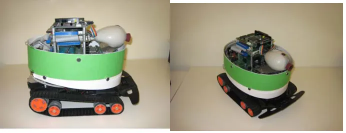
Figure #1: Example of Standard EvBot II with Green Acoustic Array
The EvBot II mobile robot platform was designed by graduate students in the CRIM [34, 44] as a test-bed for mobile robot experiments. The main processing unit is a PC-104 stack, which is mounted on a tracked Radio Controlled (RC) car body. Two BasicX microcomputer stamps control the servos used to move the tracks. A webcam is mounted on the front of the robot that gives it a field of view of approximately 40 degrees and an acoustic array can be fitted around the robot so that it can detect sound sources [3]. For this research all of the processing was done on one of the PC-104-MZ stacks on one of the EvBot II platforms. This is the slowest processor being used by the CRIM and operates at only 100 MHz. It is also limited to a 500MB flash disk and 64 MB of RAM.
3.2 Omnidirectional Camera Tower
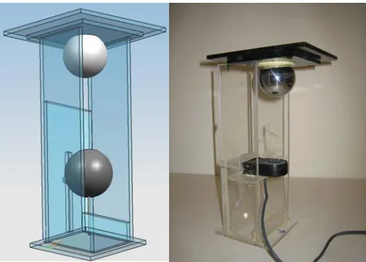
The omnidirectional camera tower was constructed of Plexiglas such that it mounted on the standoffs of the PC-104 stack that already occupied the top of the EvBot II platform. A webcam mounted inside the tower looking up a shiny sphere that would be used as the
convex mirror. Although a spherical mirror isn’t the most efficient choice for a
catadioptric system it is the cheapest option that was found (see Appendix A for detailed expense information).
Figure #2: Original Design of Omnidirectional Vision Tower (left) and Finished Tower (right)
The USB hub on the EvBot allowed for both webcams to be connected at the same time, although this did reduce the frame rate on both cameras some since they were sharing the same serial bus. The webcam was mounted on a groove such that it could be adjusted to different positions to allow the same mount to work for many different types of webcams. After the final webcam was chosen the tower was modified to better accommodate the Notebook Camera chosen for the research. The groove was removed and the webcam was mounted on a shelf 3.75” from the base of the tower. The base of the camera tower sits 9.5 inches from the floor when mounted to the top of an EvBot without the acoustic array expansion board
.
Figure #3: Example of EvBot with OV Camera Tower
3.3 Beginning Image Experiments
Once the tower was completed test images were taken. These images showed that the OV camera tower did work and that it could image the entire EvBot Arena (see Chapter 5.1 for more details about the arena) when placed in the center of the arena. The test images also revealed that the resolution and sharpness of the omnidirectional vision images was very poor. Originally this was thought to be due to the low quality of the reflective sphere used as the OV Tower mirror, but it was soon determined that the noise was artifact of the webcams themselves.
3.4 Camera Limitations
Up until this point all images had been taken using the webcams that were originally
purchased when the EvBot II platforms were designed several years ago, Phillips PCVC620K. Although capable of capturing VGA resolution images (640x480 pixels) they lacked the sharpness required for an Omnidirectional Camera system and, more importantly, they had poor color contrast; a limitation of the CCD technology they used.
By examining the pixel colorations it was determined that the color bands all faded toward grey once they were moved about four feet away from the camera base. This meant that the effective viewing distance of the omnidirectional camera was limited to less than half of the EvBot Arena. This was determined to be too limited for the OV system, to be useful a new webcam was needed. After an extensive search a new camera, the Logitech Deluxe Notebook Webcam, was found that had much better image quality. The new Logitech webcam was a bit more expensive than the older cameras at $50, but it was cheaper than most of the current generation webcams. Also, the Logitech Deluxe Notebook Webcam was a V4L device so it would be compatible with the current OS of the EvBot II platform. Base images were taken with both the old camera and the new camera.
Figure #4: Example Images from Omnidirectional Vision Tower with Old Camera (left) and New Camera (right)
3.5 Tower Modifications
The original camera towers had been designed for webcams that were designed to sit on a full-size monitor. In most of those camera designs there is a threaded socket at the base of the camera, which was used to bolt the camera to the groove in the tower. The
Logitech Deluxe Notebook unfortunately was designed to clip onto the outer edge of the display of a laptop computer. This meant that it didn’t fit well into the original OV tower so the design had to be modified. The first modification was to place a Velcro strip over the groove in one of the towers and to create a sled that would adhere to this Velcro to make the camera adjustable. This set-up can be seen in the image above (Figure 2). This configuration worked well enough to get sample images, but it had some problems. First, the camera moved too much on the Velcro strip so if the EvBot was jostled around the camera would no longer be pointed at the center of the mirrored sphere. Second, the top two inches of the Velcro blocked the view of 2 square feet directly behind the robot. The tower was modified again to remove the top two inches of Plexiglas and permanently fix the camera to a shelf 3.75” above the tower base. At this point there was the option to drop the height of the camera tower down such that the webcam would be sitting just above the PC 104 stack reducing the height of the OV tower by approximately four inches. Although this would have made the EvBot more compact several quick
experiments showed that it would reduce the overall viewing area of the OV system by a meter in each direction. Therefore, in order to view the entire EvBot arena at once the camera tower was kept at its original height.
Figure #5: Examples of Images with EvBot in the Center of the EvBot Arena (Left) and Toward the Edge of the Arena (Right) with Three Targets
3.6 Vector Angle
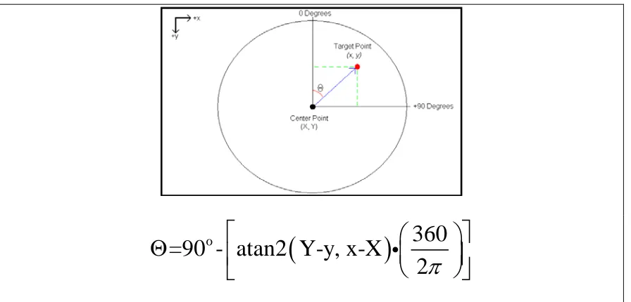
The advantage of using an axial symmetric mirror is that the angle information isn’t distorted. This means that if a target is found to be 45 degrees to the right of vertical from the center of the image then that target is 45 degrees to the right of the front of the EvBot. This made it easy to calculate the angle that a target is away from the camera base. The following equation was created to quickly determine the angle of a target pixel from this center point with relation to the pixel numbering.
(
)
o
360
=90 - atan2 Y-y, x-X
2
π
⎡
⎛
⎞
⎤
Θ
⎢
⎜
⎟
⎥
⎝
⎠
⎣
i
⎦
Figure #6: Angle Calculation for Target in OV Image in relation to host’s heading
This equation maps objects on the right hand side of the camera host to positive 1 through positive 180 degrees and objects on the left hand side of the camera host to negative 1 through negative 180 degrees. This convention was chosen to make it easier for a user to interpret the angle. If the host robot needs to face the object its direction of rotation is only dependant on the sign of the angle to that object (clockwise for positive angles, counter-clockwise for negative angles) and the angle of rotation is the same as the angle to the object (e.g. if an object is at +34 degrees the host robot needs to rotate clockwise 34 degrees to be facing it). This convention does however cause problems when an object is directly behind the host. Although negative 180 and positive 180 degrees would both work in most cases it was decided to have the negative mapping stop at -179 degrees to avoid potential problems. This also turned out to fix an issue with the Count & Out algorithm, which is discussed in Section 4.7
3.7 Camera Calibration and Distance Look-up Table
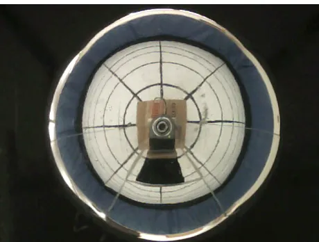
In order to determine the distance to the targets found in an image a look-up table was created. It was decided that a true camera calibration could be avoided if a look-up table could be determined experimentally so that any camera “fish-eye” characteristics would be compensated for. A calibration pattern of concentric circles spaced one foot apart with radial lines was laid down in the EvBot arena. The camera tower was placed in the center of this pattern and the following image was taken.
Figure #7: Calibration Image with Concentric Circles set 1 ft. apart
Since the OV tower mirror is spherical the concentric circles in the calibration pattern appear as concentric circles in the image. Each line represents a one foot separation so the distance from the center of the image to a line gives the vector length in pixels corresponding to the physical distance away from the camera base. Note that the resolution at the edges of the disk causes the one inch thick lines to fade into the white background and that the center of the image is dominated by the camera in the OV tower. This shows two of the limitations of this system that are discussed in more detail in Chapter 4. Due to the low resolution points along the circle were manually gathered from the picture. The points were chosen along the radial lines of the calibration pattern in order to insure that they were all in line with one another.
Vector Length to Distance 0 50 100 150 200
0 1 2 3 4 5 6 7 8
Distance from Camera (ft)
Di stan ce fr o m C e n ter o f F ram e ( p ix el s)
Figure #8: Raw Data Points for Calibration from Pixels to Distance in Feet from Host EvBot
Reviewing this data showed that there are small differences in the vector lengths
depending on what angle is being measured. It was determined that this error was due to the camera being misaligned in the tower by only 1/4 of an inch. That such a small misalignment would cause such a variance in the distance calculation showed how sensitive the Omnidirectional Camera system is to misalignments. In order to avoid future issues the camera was attached to the camera shelf with foam tape and also during this modification the back of the tower above the camera was removed since it was blocking out a significant about of area behind the EvBot. Another calibration image was taken in order to get good data points for the look-up table.
Avg. Pixel Vector Length to Distance
0 20 40 60 80 100 120 140 160 180
0 1 2 3 4 5 6 7 8
Distance from Camera (ft)
D ista n ce fr o m C e n ter o f F ram e t o D ist an ce ( P ixe ls)
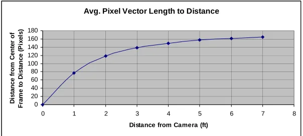
Figure #9: Line fit to data after misalignment was fixed for relationship between distance in pixels and distance in feet.
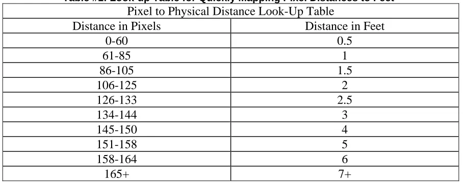
This shows that as the object gets further out on the disk (further away from the camera platform) that smaller changes in vector length translate into much larger changes in physical distance. There is good distance resolution within four feet of the camera, but beyond that the confidence that a target is at that distance is reduced. Therefore, this OV system is good for finding out roughly where targets might be located, but not at
pinpointing them exactly. This is especially true the further away the target is from the camera. Due to this resolution issue the look-up table was set-up as a bin system with more bins for the closer locations.
Table #1: Look-up Table for Quickly Mapping Pixel Distances to Feet
Pixel to Physical Distance Look-Up Table
Distance in Pixels Distance in Feet
0-60 0.5 61-85 1 86-105 1.5 106-125 2 126-133 2.5 134-144 3 145-150 4 151-158 5 158-164 6 165+ 7+
Chapter 4
Machine Vision Algorithms
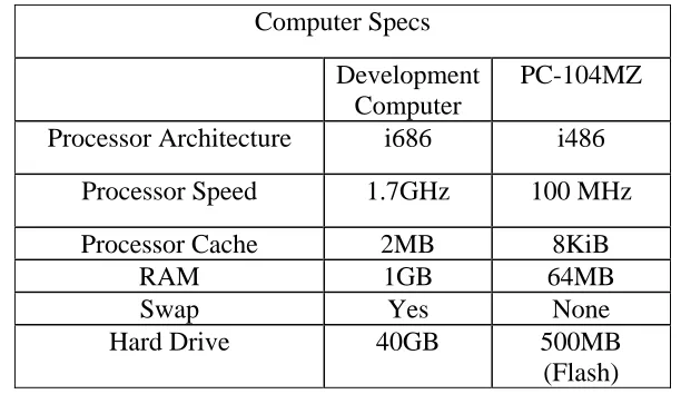
Adding an OV camera is only useful if data can be easily extracted from it and made available to the other routines running on the robot system. Machine vision algorithms were needed to take the raw images and extract the useful information. There were two main obstacles to performing machine vision techniques onboard the EvBot, limited processor power and limited RAM. The EvBot used for this research had a PC104-MZ stack as the main processor for the robot. This PC-104 stack ran a striped down version of Red Hat Linux with USB capabilities. Due to the limited processing power of the PC104-MZ native to the EvBot most of the development was run on a faster development computer and then once the code was working was moved over to the EvBot for testing. Figure 4.1 shows the primary specifications for both the Development Computer and PC-104MZ. For more complete statistics on the EvBot please reference [34].
Table #2: Computer Hardware Comparisons between Development Computer and Processor Native to EvBot II Platform
Computer Specs
Development Computer
PC-104MZ Processor Architecture i686 i486
Processor Speed 1.7GHz 100 MHz
Processor Cache 2MB 8KiB
RAM 1GB 64MB
Swap Yes None
Hard Drive 40GB 500MB
(Flash)
Obviously the development computer was able to run much more complex algorithms in real-time than the PC104 stack. Run times were recorded for the Development Computer and on the EvBot II in order to have some data for extrapolating suggested upgrades for the next generation of EvBots. This data will be presented and discussed in the
conclusions section of this chapter.
As discussed in Chapter 2, many of the OV techniques currently being used by other researchers are designed to run on much more powerful systems. Since this OV tower software is supposed to run in the background at a low priority providing OV data to other more important evolutionary algorithms the OV machine vision techniques needed to be simple and fast. Also, since the OV software was running at a relatively low priority it this software could not assume that it would be able to get sequential frames from the webcam. This meant that many of the more complicated machine vision algorithms would not be feasible for use here as they would take far too long to compute or, in the case of optic flow, require that the camera gets frames on dependable time intervals. Along with the limited processing power native to the EvBots a second problem encountered was the lack of image resolution. The OV Tower’s webcam is providing images that are 640 by 480 pixels, but only a 440 pixel disk worth of those pixels are actually looking at the mirror.
In addition to the loss of pixels around the edges there is a sizable block of pixels in the center of the image that only show the reflection of the EvBot and camera. This center section of pixel was removed from the image by a quick routine that overwrites data with a constant blue color that is close to the background color of the arena. This fixed a
problem of the machine vision algorithms finding false positive hits on the host EvBot. Once this center section is removed from the larger disk the remaining ring of pixels contains only about 44% of the pixels from the original 640x480.
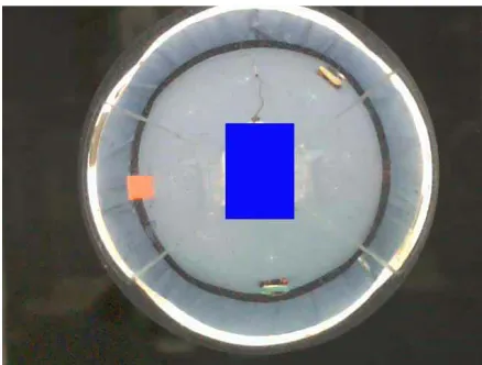
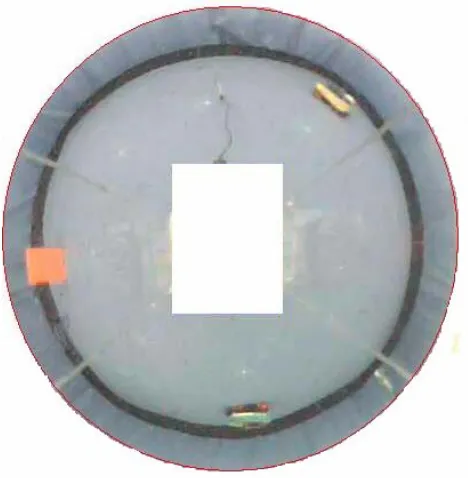
Figure #10: Example Image for OV Camera. There are three targets in the image; a yellow EvBot at 2 o’clock, a red target at 9 o’clock, and a green EvBot at 6 o’clock. The blue
square in the center masks out the camera.
This means that of the starting 302,700 pixels in the 640x480 image only approximately 133,000 pixels contain all the information for an area approximately 8 foot radius around the camera system (~200 sq. ft.). This has effectively down sampled the image by almost a third and increased the amount of area viewed by twelve and a half times (this is
assuming that the useful viewing area of the OV camera is an eight foot radius with area for the first foot removed compared to a normal camera with a 45 degree Field of View that extends out eight feet). From this it is easy to tell that the resolution, especially at the edge of the disk, is going to be a limitation. It was decided to do all of the machine vision processing on the distorted “disk” image from the OV camera rather than attempt to transform the distorted OV image into a rectangular panoramic image. This saves some processing time and allows for quicker searches. On the downside it means that many edge detection algorithms will not be applicable, due to them being optimized for horizontal and vertical lines. This isn’t seen as a disadvantage since the resolution in
many of the OV image regions is so low that most of the high frequency components that the edge detection algorithms look for are lost. The low resolution of the OV camera system effectively acts as a low pass filter.
Figure #11: Example of the Useful Pixels from the Previous OV Image
4.1 EvBot Arena
The EvBot arena is a 156.25 square foot section of the CRIM (12.5 ft by 12.5 ft square) that is the controlled environment for the EvBot II platforms. It is bordered by black walls ten inches tall with blue sheeting behind them extending up to five feet. The floor of the arena is covered with light blue plastic that provides good traction and a constant color. The arena is lit from above with indirect lighting to evenly illuminate the arena and reduce shadows. There is a camera mounted above the arena that can be used to record the EvBot movements and interactions. Due to the controlled nature of this arena it was possible to make a machine vision program very efficient by making several assumptions:
1. The light blue color of the backdrop and floor would not be used by anything else in the arena and could thus be ignored.
2. Only obstacles would be black (Including arena walls)
3. Each EvBot would have a colored band 4 inches tall around its acoustic array. 4. The colors of the bands would be known and unique.
4.2 EvBot Colors
Previous researchers [3, 34, 44] used red and green as the two distinct colors for the different EvBot teams. It was decided in this research to add a third color, one that is unique under a wide range of arena configurations. Due to the indirect lighting of the EvBot Arena most colors stay fairly consistent with position. The main issue became finding a color that didn’t fade into any of the other colors when viewed with the OV camera. The low resolution caused all colors to fade toward grey the further the target was from the camera. Since blue was already dedicated to the arena floor, black for the arena walls, red and green for the EvBots there weren’t very many choices. The only open colors were in the ranges of orange to yellow and some purples between red and blue (See Figure# 12).
Figure #12: Color Wheel with Known Targets and Unused Areas Marked
Since there was a large space in the yellows and oranges it was decided to try to find an acceptable color in that range. Samples of different colors were put in the arena and finally a bright yellow was chosen.
Figure #13: Example of Yellow EvBot in Arena as Seen by the OV camera (left) and a close-up of the Yellow EvBot outside the arena.
4.3 Machine Vision Code
Using these assumptions a simple machine vision program was written in C that could detect various objects of known colors. The programming language C was chosen because it was known to execute quickly and allowed for tight control of memory and processor executions. The principle was that since the arena is a controlled environment any large areas of color not associated with the walls, floor, or backdrop must be objects of interest in the arena.
4.3.1Configuration File
A configuration file was used to set many of the variables used by the machine vision algorithms. This file is read in each time the program is run so that the variables can be changed without recompiling the code. It would also be possible for another process to modify the values of the configuration file and restart the OmniVision program so that it could be dynamically tuned by the user process. More information about the
Configuration File and its required format can be found in Appendix C.
4.3.2 Tolerance Values for Input Targets
Each target read from the configuration file contains values for Red, Green, and Blue and a tolerance value. The tolerance value becomes one of the most important variables for all of the machine vision algorithms. Due to the camera’s innate resolution problems all colors fade toward a bluish gray as the target moves further from the host EvBot. This is due to the color data now being mapped to the pixels at the edge of image disk and
receiving fewer pixels the further away it gets. The tolerance value for each target is used by all of the algorithms in finding target pixels. Every algorithm uses the same function for pixel comparison (see below).
. . . & &
. . .
. . .
pixel red target red target tolerence if pixel green target green target tolerence
pixel blue target blue target tolerence
⎛ − <
⎜ ⎟
− <
⎜ ⎟
⎜ − < ⎟
⎝ ⎠
& &
⎞
This means that a “Low” tolerance is very strict whereas a “High” tolerance value is very lenient on which pixels count as targets. The software doesn’t check the input values and the tolerance for collisions so poor choices for tolerance values will mean that an object in an image will be identified multiple times as different targets. It also means that if the tolerance is set too high the color space will include the background blue color for the arena. An example of a tolerance value that is too high is shown below, see Figure #14. All of the green pixels are ones marked as target pixels. It shows that there are lots of false positives, especially on the walls of the arena, but that it did find all of the pixels on the color band.
Figure #14: Example of Setting Tolerance Value Too High. The Green Target is at 2 o’clock and all the other green pixels are false positive hits found by the software.
4.3.3 Trimming Targets
An issue that arose during many of the experiments with the Region Growing Algorithm (see section 4.4) was that small groups of false positive hits were grown. These
erroneous blobs were usually on the curtains that form the walls of the arena or on the floor of the arena. In both cases they were usually less than ten pixels. Other than the size of the blobs the false positives were inconsistent and depended greatly on the lighting around the arena. A trimTargets() function was created that removed any targets with a connected region count less than a certain pixel count. Some rough experimentation showed that setting the threshold at 10 pixels removed the vast majority of the false positive hits without negatively affecting true positive results.
4.3.2 Webcam Set-Up
After this configuration file has been read in by the OV program upon start up it is stored in an InputSettings struct (See Appendix B for software diagram and struct definitions) where it is handed to all of the algorithms as they need the information. Software was written that sets-up the webcam such that it functioned in RGB mode. There were many driver problems that occurred while trying to get the webcams working on the PC-104 boards running the Linux OS. A more detailed discussion about the driver problems can be found in Section 4.4.3. Forcing the webcam into RGB mode meant that the extracted frames were already in the correct color format and were stored in a file buffer. The webcam software also read in each frame as a file buffer and only saved images to jpegs when specifically requested by the user. Both of these features allowed the software to run quicker, while giving the operator flexibility on getting images from the system at
different points in the process (See Appendix C for more information about getting images from the camera). The software also overwrote all of the pixels in the center of the image where the camera and host EvBot are located (See Figure #10) These pixels were all made to be a blue very close to the color of the EvBot Arena floor so that they wouldn’t be picked up by any of the machine vision algorithms. This fixed the problem of the machine vision algorithms getting false positive matches due to the color of the EvBot circuit boards being very close to the color of the green EvBot targets.
4.4 Region Growing on Unmodified OV Image
Due to the constraints on the EvBot system discussed earlier the machine vision
algorithms would need to be very simple in order to run in a timely manner. Most of the higher frequency data in the images (sharp lines) is lost due to the resolution issues inherent to an omnidirectional camera. Also, since most of the defining data for the targets of interest is color data the frequency based algorithms, such a sliding window FFTs, were abandoned for functions that find connected color regions. For these reasons a Region-Growing algorithm was applied first. The Region Growing algorithm searches an image for a pixel that matches one of the entries in the configuration file (allowing for that entry’s tolerance value). Starting from that pixel it performs an 8-neighbor search for other pixels that match that particular entry. As the program found pixels that matched that entry they were added to an array list for that region and that pixel’s neighbors were then explored. Eventually this method finds all of the pixels that belong to a connected region of color. The centroid of this region would then be calculated by averaging all of the pixel coordinates. This centroid is then used to compute the distance
of the region from the center of the image using a look-up table. This distance should be the distance from the EvBot to the center of the target.
4.4.1 Binary Images
The major disadvantage to using a region growing algorithm is the number of
comparisons that need to be made and the bookkeeping that has to occur that keeps track of which pixels are in the individual connected regions along with which pixels have already been searched. Not only does each pixel in the image need to be checked to see if it falls into a one of the target color bins (one comparison each for Red, Green, and Blue values for each pixel), but a standard region growing algorithm could examine the same pixel up to eight times. Since there are 302,700 pixels in a standard VGA
resolution (640x480) image this could result in so many comparisons that the algorithm runs very slowly, especially on the EvBot. Not only is the number of comparisons very high, but each comparison involves an absolute value operation, which is often very computationally expensive. To combat this obstacle Binary Images were created for each target in the configuration file. Each Binary Image is created such that it has a single bit for each pixel in the image. It does all of the comparisons for every pixel in the image for a specific target value. If a pixel falls into one of the target bins then its bit in the Binary Image is raised. This allows for the expensive absolute value comparisons to only need to be done once per pixel per input target and since binary comparisons are very quick this also helped speed of the Region Growing Algorithm. This has the added effect of reducing the memory footprint for each image from 921,600 bytes for raw RGB888
format to 38,400 bytes per Binary Image. In most cases there were three targets in the input file so the memory was effectively reduced by 3.
4.4.2 Experimental Results from Region Growing on Unmodified Image
The Region Growing algorithm was run for many different arena configurations. It was able to successfully find the targets, but it was noted that it often found multiple blobs per target.
Figure #15: Full OV Image with Trimming. Grown Regions are Shown as Black Pixels Overlaid with Original Image
In Figure #15 above the solid black pixels are the ones that the Region Growing algorithm found and grew. It is easy to see that both the red and green targets were detected as two separate connected regions. Also since the target list is still being trimmed at this point the algorithm may be growing more connected regions that are below the trimming threshold.
Figure #16: Examples of the Red Target (left), Green EvBot (middle), and Yellow EvBot (Right) with the grown regions highlighted in black. Note that both the Red Target and Green EvBot have two distinct and disconnected regions. Also note that this is with any
blobs under 10 pixels being trimmed.
It was determined that this type of separation of the targets was caused by the curved surface of the color bands around each EvBot reflecting the light in slightly different manners. To try to fix this first the trimming algorithm was disabled. The results from that are shown below.
Figure #17: Same Image as Figure #15 without Trimming. Note the false positive hits at the bottom of the image on the walls of the arena.
Figure#18: Targets Extract from Figure #17 with Grown Regions Indicated in Black. Note the false positive hits around the green EvBot and especially on the red wheel.
This shows that although some of the dropped regions were on the correct targets there were many false positive hits that trimming had removed. Of particular interest is the false positive hit on the wheel of the green EvBot in Figure #18. With trimming turned off this run would have reported that a red target was collocated with the green EvBot. This shows that the trimming function does keep the number of false positive hits down, but that it also means that the algorithm might throw away useful data. It was determined that the trimming algorithm was needed to avoid false positives so the tolerance value was increased to 35 to see if it found more connected regions.
Figure #19: Region Growing on Raw Image with Tolerance Moved from 25 to 35
Figure #19 shows quite well that raising the tolerance value won’t work for connecting the blobs since it results in so many false positive hits. It can also be seen that with higher tolerance values the shadows of the EvBots, although minimal due to the over head indirect lighting, do cause false positive hits (this is most notable around the base of the green EvBot in Figure #19). To further examine the effects of the tolerance values to finding the target EvBots an experiment was performed with the tolerance set to 15 instead of 25. This experiment resulted in no targets being found thus showing how sensitive the Region Growing Algorithm is to target tolerance values. A tolerance value of 25 finds only the desired targets (although there are often multiple disjointed regions in each target), but a tolerance deviation plus or minus 10 results in completely unusable results.
4.4.3 Execution Time Analysis for Region Growing
After showing that the region growing algorithm would work with the OV camera and tuning the tolerance values properly the software was compiled on the EvBot II and run on the 100 MHz processor native to the robot. It was noted that on the Development Machine (see Table #2 at the beginning of Chapter 4) the Region Growing algorithm took approximately 150 milliseconds to process a single frame without saving any of the images to disk. On the EvBot the same code took over 20 minutes to process a single frame. Some profiling was done that showed that a significant amount of time (up to 40 seconds) was being used to just read the image from the camera, but that if just the camera code was run (removing all of the Region Growing code) it took on average 3 seconds to read each image. It is unknown exactly what caused this discrepancy, but the
most likely cause is the webcam driver. The Logitech Deluxe Notebook webcam uses the SPCA5XX driver to work with Linux. It was noted that the driver was only
marginally supported on the i486 architecture. Improving either the EvBot II processor or the webcam driver may fix the image read time issue. It was estimated that the Development Computer would run code at least 150 times faster than the EvBot processor (1.7 GHz vs 100 MHz). With this estimate in mind it was expected that the EvBot would run the Region Growing code in about 1 minute. After removing the read times a comparison showed that the Development Computer actually ran the code 600 times faster than the EvBot. At this point it was determined that the EvBot could never actually run any machine vision algorithms in real time, let alone have them run as a background processes. This data could be used however to show what processor any upgraded EvBot II would need in order to have a chance at running machine vision algorithms onboard. It was also noted that the images could be passed off the EvBot II platform via the wireless 802.11b link so that these algorithms could be run on faster desktops.
4.5 Region Growing after Image Closing
Although Region Growing was shown to be rather slow it was also shown to be effective at finding the targets accurately when properly tuned. One issue that was noted with Region Growing was that it often grew several disconnected regions on each target (see Figure #16). Each of these different regions would be reported back as a distinct target. Although the user could likely tell when targets were collocated some experiments at filtering the image prior to the Region Growing algorithm was attempted to see if the regions could be merged.
4.5.1 Definition and Discussion of Closing
The first filter that was used was Closing, which is defined as dilation and then erosion by the same structuring unit. In this case a 3x3 block was the structuring unit. It allows for target blobs to merge if they are within one or two pixels of each other.
4.5.2 Dilation
Dilation is one of the basic binary morphology operators [48] where each target pixel is dilated by the structuring element. The formal definition of Dilation is[48]:
(
)
{
}
:
|
,
b b B
Dilation of A by B
A
B
a b
a
A b
B
which is equivilent to
A
B
A
∈
⊕ =
+
∈
∈
⊕ =
∪
In the case of a 3x3 structuring element this grows a connected region by one pixel in every direction (see Figure #20 below).
Figure #20: Example of Dilation using 3x3 Structuring Unit
4.5.3 Erosion
Erosion is one of the other basic binary morphology operators and is the opposite of Dilation. The formal definition of Erosion is:
(
)
(
{
}
:
|
,
b b B
Erosion of A by B
)
A
B
a
a b
A for every a
A b
B
A
B
A
∈
Θ =
+ ∈
∈
∈
Θ =
∩
For this application, using a 3x3 structuring unit, Erosion shrinks the connected region by one pixel in every direction (see Figure #21 below).
Figure #21: Example of Erosion using 3x3 Structuring Unit 4.5.4 Closing
Closing a binary image therefore will result in bridging gaps internal and between connected regions. The size of the gaps bridge depends on the structuring element used, in the case of a 3x3 structuring element it can bridge gaps of 2 pixels (see Figure #22 below). The main advantage of performing closing is that it only adds the bridging pixels to the overall image as long as the same structuring element is used for both Dilation and Erosion.
Figure #22: Example of Closing Using 3x3 Structuring Element
4.5.5 Experimental Results of Region Growing on Closed Image
Experiments were run that Closed the image with a 3x3 structuring element prior to performing the Region Growing algorithm.
Figure #23: Example Image with Standard Tolerance after Closing Image
Figure #24: Targets from Figure #23. Red Target (left), Green EvBot (middle), and Yellow EvBot (right)
These experiments showed that the Closing operator did combine some of the
disconnected regions in some of the targets, but that the gaps were in many instances greater than two pixels. A few experiments were run trying larger structuring elements, but the number of false positive errors increased dramatically. Also, run-time analysis showed that the Closing operator was very processor expensive. On the Development Machine it doubled the time to process a single frame, taking it to ~0.4 seconds per frame. On the EvBot Closing the image added on average about 3 minutes to the processing time, but this was only about a 10% increase in the overall runtime. It is suspected that the smaller cache on the i486 architecture lead to the actually region growing being much more inefficient than on the development computer. Using the profiling program ValGrind it was determined that the Erosion operator was significantly more complex than Dilation. This is reasonable since for each pixel in the region Erosion checks all of its neighbors before deciding if that pixel is to remain. It was thought that perhaps the Erosion step in the Closing process could be eliminated to help improve run times.
4.6 Region Growing on Dilated Image
A series of experiments were run that Dilated the image by the 3x3 structuring element before Region Growing was attempted on them. Figure #25 and Figure #26 below show an example of one of these runs.
Figure #25: Example of OV Image with Dilation
Figure #26: Targets from Figure #25.
Red Target (left), Green EvBot (middle), Yellow EvBot (right)
4.6.1 Experimental Results of Region Growing on Dilated Image
These experiments showed that Dilation of the image prior to Region Growing improved the Region Growing algorithm’s success rate of finding pixels on the color bands of the EvBots, but also it resulted in a large number of false positive hits. These false positive hits were not removed by the trimming since Dilation had caused their size to be larger than the 10 pixels effective in trimming the previous two sets of experiments. Increasing the trimming threshold resulted in most of the false positive errors being removed. A user could also remove extraneous false positives by limiting the distance a target can be from the host since many of the remaining false hits are on the curtains around the EvBot. Removing the Erosion step in the Closing process also cut the processing time down significantly. Run times on the Development machine were reduced from 900 ms for
Region Growing with Closing to 500 ms for Region with Dilation. Runtimes on the EvBot were likewise expedited, ~3 minutes per frame for Region Growing with Closing versus ~2 minutes per frame for Region Growing with Dilation.
4.7 Experimental Results Comparisons of Previous 3 Region Growing Experiments
After completing numerous experiments with Region Growing on the raw image, the closed image, and the dilated image it was determined that Region Growing after dilating the binary image resulted in the most number of pixels found on each target, but also the highest rate of false positive errors. Figure #27 below shows a side-by-side comparison of the algorithms on the same EvBot.
Figure #27: Side by Side Comparisons of Region Growing Results
Although Region Growing on the Dilated Image resulted in higher false positive errors it was decided that the user could deal with all of those errors through either a knowledge based filter or by dynamically adjusting the trimming threshold. To accommodate this the setUpOV() function, which allows the user to modify the OV and algorithm settings, was modified to allow for user control of the trimming threshold.
4.7 Simple Counting with Easy Out on Sub-Images (“Count & Out”)
After the issues involved in the region growing algorithms it was decided to try an even simpler algorithm. The image is broken up into 16 by 16 pixel blocks so that a 640x480 image is effectively down sampled to 30x40.
Figure #28: Full OV Image divided up into 16x16 pixel blocks
The “Count and Out” algorithm takes each block and counts how many pixels fall into each target bin. If any bin count reaches a threshold that is set in the configuration file then the entire block is allocated to that target. After a first pass where all the SubBlocks are sampled the distance and angle for each block that is a target hit are calculated. This often results in numerous vectors toward a single target. In the sample below the
algorithm returned hits on five of the SubBlocks.
Figure #29: Example of EvBot distributed over 16x16 pixel blocks
The list of hits is then merged such that any vectors that fall within a set angle and a set distance (both of which are read in from the configuration file) of the same target ID are merged into a single vector. This pass is only done once to avoid merging distinct targets and so the algorithm can be used to track wall locations.
4.7.1 “Count & Out” Tuning
The effectiveness of this algorithm is dependant on four separate variables aside from the color of the target. These variables are MaxCount, MaxAngle, MaxDistance, and target Tolerance. Of these variables target Tolerance is the only one that varies between the individual targets. The MaxCount variable is how many pixels in each 16 by 16 pixel block need to be within a single target bin before the entire SubBlock is allocated to that target. The MaxAngle and MaxDistance variables are used in the merging function to decide how to merge the many hits a single target often has. If the Tolerance on a target color is too high then false positives will occur from various reflections around the EvBot arena. If the tolerance is chosen too low then there won’t be enough pixels in a bin to have any SubBlocks allocated to any colors. If the MaxCount is lowered the algorithm becomes very susceptible to noise in the image, which results in false positive results. If
MaxAngle is set too high then two separate targets near each other will be merged into a single target, while if it is set too low the merging will be incomplete and a single target may have two or more vectors still pointing to it after the merging algorithm. If
MaxDistance is too high then targets that are behind another target of the same color will be merged with the close target, while if it is too low the merging function won’t function properly.
4.7.2 Count & Out Trade Offs
The count and out algorithm can be remarkably efficient under certain situations. Unlike for Region Growing this algorithm will only touch each pixel once and, since it exits the counting process once the threshold is reached, it will often not have to compare every in an image. This makes the algorithm more efficient the more targets are in the image. The drawback is that “Count and Out” doesn’t maintain any sense of connected regions. It can easily merge two different targets of the same color if they get too close to each other. It will also give multiple hits to any large area. The advantage to the multiple hits for any large targets is that it could be used to track the walls of the EvBot arena as well as the location of targets.
4.7.3 Experimental Results of Count and Out Algorithm
The “Count and Out” algorithm was run on the same arena arrangements as the previous three experiment sets and performed very well. It was noted that since the counting threshold was set around 25 pixels it had very few false positive hits, but still found the targets with comparable accuracy to the Region Growing algorithms. It was also noted
that with the merging angle set to around 15 degrees there were very few instances where a single target had multiple hits. The main observation about the “Count and Out” algorithm was that it ran very quickly; taking around 19ms per frame to run on the Development Machine and around 40 seconds per frame to run on the EvBot II. This dramatic speed increase compared to region growing does come at the expense of
accuracy since it has no real concept of connected regions. For most arena situations this didn’t cause any problems, but several experiments were performed where two EvBots of the same color were placed next to each other in the arena. The Region Growing
Algorithms always returned that there were two targets, but the “Count and Out” algorithm would often merge the two targets into single hit. Also several experiments were preformed where a very large target was placed very close to the camera host. In these experiments the “Count and Out” algorithm always resulted in multiple hits to the same target. This could be countered by increasing the merging angle, but in doing so distinct targets further from the host would then be merged. It was decided that a merging angle of 15 degrees and a merging distance of 100 pixels was a good
compromise that worked well for the vast majority of expected arena situations. Also of interest was that if the black color of the edges of the arena was added to a input target list the “Count and Out” algorithm could track the arena edges. It would return a fairly even spread of vectors from the host to the edge of the arena approximately equal to the merging angle (see Figure #30).
Figure #30: Simulated Example of Arena Boundary Tracking
It was also noted that this didn’t greatly increase the execution time of the algorithm. Examining the program flow in more depth showed that the “Count and Out” algorithm became more efficient the more crowded the arena became. This was due to the fact that the “Count and Out” algorithm would stop making comparisons as soon as the count threshold was reached, hence the title of the algorithm. A 16x16 pixel block contains 256 pixels. Each pixel has three color values such that the worst case scenario of completely comparing all three pixel values for every pixel in a SubBlock would be 768 comparisons and absolute value calculations. If the first 25 pixels, the recommended count threshold, are all matches to a single target then the algorithm saves 693 computations (granted this is the best case scenario). Overall, the worst-case number of comparisons for the “Count and Out” algorithm is equal to the required number of comparisons to make a single Binary Image for one target value in the Region Growing algorithm. The more targets that are found the fewer pixel comparisons need to be made, but the greater the number of atan2() calls and the time to merge the targets goes up. Exactly what this relationship is wasn’t explored due to time constraints, but the “Count and Out” algorithm showed that it is by far the superior algorithm for this OV implementation.
4.8 Side-by-Side Comparison of All Algorithms
After testing the Count and Out algorithm runtimes were compared for all of the
experiments looking at a standard arena configuration (3 targets each of a separate target color arrange around the camera host between 3 and 6 feet away, see Figure #31).
Figure #31: Standard Arena Configuration used for Execution Time Comparison Experiments
The results of the execution time experiments can be seen in Table #3 below.
Table #3: Execution Time Comparisons
Action Development Computer Execution Times
(average time in seconds)
EvBot Execution Times (average time in seconds) Read Image from WebCam 0.067 5.5
Convert from File Buffer to Image Struct
0.0046 7.6 Count and Out Algorithm 0.015 23.1
Region Growing on Raw Image 0.147 1363 (22 min, 43 sec) Closing Image 0.153 162
(3 min, 42 sec) Region Growing on Closed
Image
0.096 735 (12 min, 15 sec)
Dilating Image 0.079 64 (1 min, 4 sec) Region Growing on Dilated
Image
0.784 1395 (23 min, 15 sec)