ABSTRACT
BARGE, WALTER S. II. Autonomous Solution Methods for Large-Scale Markov Chains. (Under the direction of William J. Stewart.)
AUTONOMOUS SOLUTION METHODS
FOR
LARGE-SCALE MARKOV CHAINS
by
WALTER S. BARGE, II
A dissertation submitted to the Graduate Faculty of North Carolina State University
in partial fulfillment of the requirements for the Degree of
Doctor of Philosophy
OPERATIONS RESEARCH
Raleigh
2002
APPROVED BY:
You may say to yourself, “My power and the strength of my hands have
pro-duced this wealth for me.” But remember the Lord your God, for it is he who
gives you the ability to produce wealth, and so confirms his covenant, which
he swore to your forefathers, as it is today.
Biography
Walter Shepherd Barge, II, was born in the Army Hospital at Fort George
G. Meade, Maryland. He is one of three brothers and the eldest son of Sarah
Patterson Barge and Walter Shepherd Barge, Sr. He grew up as an army
brat and graduated from James I. O’Neill High School in Highland Falls, New
York. In 1982 he graduated Magna Cum Laude from North Carolina State
University with a Bachelor of Science in Civil Engineering and accepted a
commission in the United States Army.
After tours of duty in Hawaii and Germany he attended the Georgia
In-stitute of Technology where he earned a Master of Science in Operations
Research. These studies were followed by teaching undergraduate
Mathe-matics at the United States Military Academy, West Point, NY.
From 1994 to 1999 he served with the 577th Engineer Battalion, Fort
Leonard Wood, Missouri; in the Former Yugoslavia during Operation Joint
Endeavor; and on the faculty of the Army War College, Carlisle Barracks,
Pennsylvania. In 1999 he was assigned to the Army Student Detachment to
begin his Ph.D. studies at North Carolina State University. He is currently
on active duty at the rank of Lieutenant Colonel.
He is married to the former Sarah Kathryn Armstrong and they have one
Acknowledgments
I owe a debt of gratitude to Dr. Billy Stewart for his guidance, patience and
encouragement. Without his expert insights I would not have been able to
complete this research. I am also grateful to Drs. Thom J. Hodgson, Russell
E. King, and Robert St. Amant for giving their time and talent to serve on
my committee.
I am also indebted to fellow Ph.D. students Amy Langville, Emily Lada,
and Edna Chan who made the rigors of graduate school interesting and
enjoyable. Amy and I had many discussions on the theories and techniques
of solving Markov chains and they always ended with greater understanding
on my part. I also need to thank Gary Gatling, Jason Askew, and Reuben
Stocks of Information Technology and Engineering Computing Services for
their responsive computer support. I wish them all continued success.
I would like to thank the United States Army for the lifetime of education
they have provided to me. Every college opportunity I have undertaken has
been supported by the Army—either financially or with duty time to attend
classes. I strive to repay these opportunities with sincere efforts on behalf of
the Americans who pay my salary.
Finally, I thank my wife, Sarah, and daughter, Kathryn, for their love,
encouragement, and cheerful attitudes during this effort. My “second”
grad-uation from NCSU will coincide with our 20th wedding anniversary—I could
Table of Contents
List of Tables ix
List of Figures xii
1 Introduction 1
1.1 Research Motivation . . . 1
1.1.1 Possible Roadblocks . . . 2
1.1.2 Roadblock Removal . . . 4
1.2 Research Hypothesis . . . 5
1.3 Research Objectives . . . 5
1.4 Research Approach . . . 6
1.5 Dissertation Road map . . . 7
2 Technology and Literature Review 9 3 Markov Chain Concepts and Terminology 13 3.1 Example of a Markov Chain . . . 14
3.3 Definitions and Terminology . . . 18
4 Solution Methods 25 4.1 Direct Methods . . . 26
4.2 Iterative Methods . . . 27
4.2.1 The Power Method . . . 28
4.2.2 Additional Iterative Methods . . . 31
4.3 Projection Methods . . . 45
4.4 Decompositional Methods . . . 54
4.5 Solution Methods Summary . . . 55
5 Selection of a Solution Method 58 5.1 Solution Criteria . . . 58
5.2 Battery of Initial Tests . . . 72
6 Design of the Expert System 76 6.1 Components of a Basic Expert System . . . 78
6.2 Implementation . . . 82
6.3 Example Problem for the Expert System . . . 84
7 A Proposed Graphical User Interface 87 7.1 User Interface and Software Details . . . 89
7.2 Matlab and Fortran Files . . . 91
8.1 Description of Five Test Models . . . 94
8.2 Solution Experiments . . . 100
8.2.1 Kanban Model . . . 103
8.2.2 Satellite Model . . . 109
8.2.3 Time Sharing System (TSS) Model . . . 111
8.2.4 Recurrent Epidemic Model . . . 113
8.2.5 Resource Sharing Model . . . 115
8.2.6 Summary of Solution Experiments . . . 117
8.3 Method Switching Experiments . . . 117
8.4 Scalability Experiments . . . 121
8.5 Parameter Adjustment Experiments . . . 124
9 Critique and Future Research 131 References 134 A User’s Guide 139 B Computer Code 141 B.1 Expert System matlab Code . . . 141
B.2 GUImatlab code . . . 148
B.3 Solution Methods matlab code . . . 163
B.4 Example of mex-fortran code . . . 176
List of Tables
3.1 Transition probabilities of daily fire danger . . . 14
4.1 Summary of solution methods . . . 56
4.2 Summary of IAD method . . . 56
5.1 Time estimate for Gaussian elimination . . . 71
6.1 M-files used in the expert system . . . 83
6.2 Initial test results for kanban55 Model . . . 84
7.1 Files called by the m-file m build.m . . . 91
7.2 Files called by the m-file simple gui1.m . . . 92
7.3 Files called by the m-file simple gui2.m . . . 92
8.1 State space size for satellite model . . . 96
8.2 Model parameters for kanban55 . . . 103
8.3 Initial test results for kanban55 Model . . . 103
8.4 Initial test times for kanban55 Model . . . 104
8.6 Solution times for kanban33 model . . . 106
8.7 Solution search forkanban66 model . . . 108
8.8 Model parameters for sat54 . . . 109
8.9 Initial test results for sat54 model . . . 109
8.10 Solution times forsat54 satellite model . . . 110
8.11 Model parameters forncd40 . . . 111
8.12 Initial test results forncd40 model . . . 111
8.13 Solution times forncd40 TSS model . . . 112
8.14 Solution times for TSS model . . . 112
8.15 Model parameters forridler256 . . . 113
8.16 Initial test results forridler256 model . . . 113
8.17 Solution times forridler256 model . . . 114
8.18 Model parameters formutex8 . . . 115
8.19 Initial test results formutex8 model . . . 115
8.20 Solution times formutex8 model . . . 116
8.21 Expert system method choice . . . 117
8.22 Matrix Score as a solution method criterion . . . 118
8.23 Extendkanban54 tokanban55 . . . 122
8.24 Extendmutex7 to mutex8 . . . 122
8.25 Extendncd4 toncd6 . . . 123
8.26 Extendncd5 toncd6 . . . 123
8.27 Re-use of solution vector: ridler100 . . . 126
8.29 Re-use of solution vector: ridler256 . . . 128
8.30 Comparison of vector norms: ridler256 . . . 129
8.31 Re-use of solution vector: kanban54 . . . 129
List of Figures
3.1 State transition diagram of daily fire danger . . . 15
3.2 DTMC transition diagram . . . 17
3.3 A reducible Markov chain . . . 19
3.4 An NCD Markov chain . . . 20
3.5 An example of periodicity . . . 21
4.1 Subdominant eigenvalue plot . . . 36
4.2 Golden Section adaptive ω adjustment forkanban55 matrix . 39 4.3 Convergence ratio adaptive ω adjustment forkanban55 matrix 41 5.1 Element-wise plot of mutex2 . . . 63
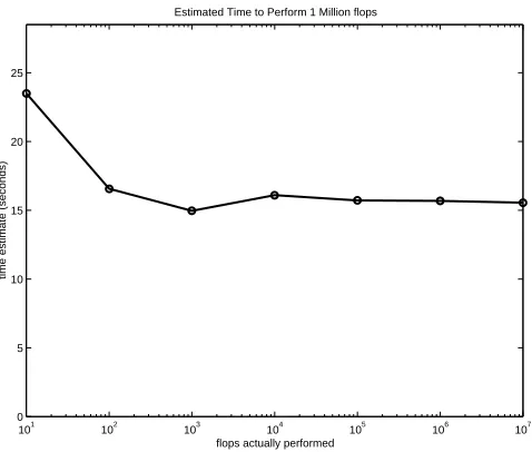
5.2 Typical time estimate plot . . . 70
5.3 Possible time estimate plot . . . 70
6.1 Sieve decision chart . . . 77
6.2 Model of a rule-based expert system . . . 79
8.1 Schematic of a kanban system . . . 95
8.2 Satellite telephone model . . . 96
8.3 Time-sharing computer system . . . 97
8.4 Epidemic model transition . . . 99
8.5 Resource sharing model . . . 100
8.6 Subdominant eigenvalue plot . . . 107
8.7 Solution vector plot . . . 127
Chapter 1
Introduction
1.1
Research Motivation
Since their introduction in the early 1900s, Markov chains have been proposed
as a means of modeling a variety of stochastic processes, including weather
forecasting, voting patterns, and demographic trends. Markov chains have
even been suggested as a model to predict and guide usage of the World
Wide Web [34].
In his book, Modeling and Analysis of Stochastic Systems [23], Kulkarni
provides some details on how applications in genetics, sociology, manpower
planning, neurology and telecommunications could be modeled as Markov
chains. In most scenarios, the models are kept very small, usually less than
several hundred states, in order to be kept tractable. The use of large Markov
knowledge of numerical solution algorithms. Subject areas where large
mod-els have been used successfully include telecommunications and computer
systems performance modeling.
1.1.1
Possible Roadblocks
The successful use of a Markov chain model involves at least three (global)
steps:
1. A detailed knowledge and understanding of the application domain
such as genetics, weather forecasting, or telecommunications.
2. A working knowledge of how to construct a Markov chain model.
3. The knowledge and ability to obtain useful information from the Markov
chain after it has been constructed.
We contend that step 3 represents a real and often unnecessary roadblock
for potential users of Markov chain modeling.
The ability to model a system or procedure using a Markov chain can be
distinct from the ability to analyze the chain’s behavior. Modeling ability
is derived primarily from a basic knowledge about the meaning of a Markov
chain coupled with adetailed knowledge of a specific application area. One of
the roadblocks to greater application of Markov chains is that potential but
non-numerically sophisticated users possess the detailed domain knowledge
deciding which numerical method might be best suited to their applications.
A realistic Markov chain model can easily contain thousands or hundreds
of thousands of states. The transition matrix can be quite sparse, which
means that compact storage schemes, which store only non-zero elements,
are often required to make the matrix manageable for the computer. The
choice of a particular solution method also has a great effect on the amount
of time required to obtain a solution. Even after deciding upon a certain
method, implementation details imposed by compact storage schemes and
the nature of the solution methods themselves pose additional barriers. As
a consequence, users may severely restrict their models to keep them small
enough so that software packages such as matlab can be used.
The difficultly with a self-imposed model size restriction is that even
small, simple models can generate very large state spaces. An example we
have used in our research is a manufacturing model proposed by Krieg and
Kuhn [22] that describes a kanban controlled production system where
prod-ucts are processed on a single manufacturing facility. With only five different
products and five kanbans for each product the resulting Markov chain has
71,280 states. Clearly, an a priori size limitation is not a realistic approach
for removing roadblocks to the usefulness of Markov chain models.
Greenbaum observes that “it remains an open problem to characterize
the classes of problems for which one [solution] method outperforms the
oth-ers” [16]. Indeed, she reports that examples can be constructed for which a
researcher’s goal. In their book, Templates for the Solution of Linear
Sys-tems, Barrett, van der Vorst, and Dongarra, et al, agreed with Greenbaum
and summarized their comments on Krylov subspace methods by stating that
“there will be no ultimate method” [5].
Because the modeling nuances are limitless we hold out little hope for a
far-reaching theoretical classification scheme that encompasses all potential
Markov chain models and the currently known solution techniques. Instead,
we take the view offered by Barrett, et al: “The best we can hope for is some
expert system that guides the user in his/her choice.” [5].
1.1.2
Roadblock Removal
Where does this leave the non-numerically sophisticated user? This person
is in need of an intelligent software tool to guide the analysis. We envision
an experimentally-validated solution approach embedded into a software
ap-plication. The application should have a suitable user interface to guide the
analysis of a Markov chain. We propose a battery of diagnostic tests to be
performed at the time the Markov chain matrix is obtained by the software.
The results of these tests are interpreted by an expert system and then a
suitable solution method is chosen and executed. In addition to selecting an
appropriate solution technique, any needed algorithm parameters are
sup-plied for the novice user.
The goal is that both the initial tests and the interpretation of their
to the analysis. Our analogy for this system is that of a sieve which receives
a Markov chain and sifts out information from the matrix that can be used
to make an intelligent solution recommendation.
Our goal in this dissertation is to show how advantage may be taken of
information readily available in the Markov chain to aid in the selection and
execution of a solution method.
1.2
Research Hypothesis
A computer tool with a graphical user interface (GUI) and embedded
knowl-edge could provide a beneficial means to make Markov chain analysis more
available to current and prospective Markov chain users. This computer
tool could receive a user’s Markov chain, examine the chain, determine its
primary characteristics, and then give the user useful information and
recom-mendations about how to analyze the model. This can be done without the
user being an expert in the various solution techniques and their respective
areas of applicability. Finally, the tool should allow users to override the
recommendation and select a solution technique of their choosing.
1.3
Research Objectives
• To determine the feasibility of using a GUI solution tool that makes
industry practitioners.
• To demonstrate implementation of a knowledge-based GUI solution
tool.
• To demonstrate that the research hypothesis is correct by examining
several real world problems and attempting to meet user needs.
1.4
Research Approach
Our research approach is divided into three broad areas.
• Conduct literature search. Areas of concentration are:
– Current and common uses of Markov chains
– Solution mechanisms (approach and software) commonly used to determine system behavior
– Similar uses of a knowledge-enhanced GUI
– Similar approaches that have been developed to make optimiza-tion more accessible
– Trends in statistical expert systems in the 1980s and 1990s
• Develop an implementation of an intelligent GUI tool to examine and
solve Markov chains. Specific issues include GUI design, Markov chain
input methodology, and detection of user’s information needs as well
• Test the GUI solution tool on several real-world problems that can
benefit from use of a Markov chain modeling approach. Determine the
limitations and/or extensions required to use the proposed GUI tool
for more widespread use on real-world problems.
1.5
Dissertation Road map
The dissertation is organized into 9 chapters.
• Chapter 2 reviews the literature and related technology efforts. Here
we show precedents for our approach and point out extensions and
contributions that we will make.
• In Chapter 3 we give an example of a Markov chain and show how they
fit into the broader framework of stochastic processes. We also define
terms that will be required later.
• In Chapter 4 we discuss in detail the solution methods used in this
research.
• Chapter 5 discusses our choice of specific solution criteria for obtaining
a solution and details our specific approach for testing Markov chain
matrices.
• Chapter 6 describes the basics of Expert Systems and details our
• In Chapter 7 we describe our Graphical User Interface.
• In Chapter 8 we describe our five test models and then present the
results of our numerical experiments using the software tool and expert
system. We also present results from Method Switching, Scalability,
and Parameter Adjustment experiments.
• Lastly, in Chapter 9 we summarize and critique our work and present
Chapter 2
Technology and Literature
Review
The ability to model a system or procedure using a Markov chain is derived
primarily from a basic knowledge about the meaning of a Markov chain
coupled with adetailed knowledge of a specific application area. Examples of
application areas are genetics, meteorology, and manufacturing. In complex
application areas the Markov chain can grow to many thousands of states,
or more.
Of course, the purpose for modeling a system, be it with Markov chains,
or any other technique, is to gain valuable information about the system.
In terms of Markov chains, this implies the ability to compute various
func-tionals, or metrics, that are characteristic to the system (as described by the
is the stationary distribution of the Markov chain. Some functionals can be
obtained by more than one method and this is true for the stationary
distri-bution. If the state space is large, the novice user of Markov chains may not
be equipped to solve the Markov chain in an efficient manner. The choice
of a solution technique can have a large impact on the speed, efficiency, and
accuracy of the computed solution. A person with experience solving Markov
chains might employ a variety of tests or judgments to reach a conclusion
about which solution technique to use. This expertise may be lacking in a
person who possesses all the abilities required to devise and construct the
model.
Basic texts that introduce Markov chains as stochastic models may even
unknowingly contribute to user confusion in selection of an appropriate
so-lution method. Some use an iterative scheme (e.g., power method) as a way
of illustrating convergence to a stationary solution but may then leave the
reader with the impression that direct methods are used for routine solution
of Markov chains [21, 44, 14, 31].
The idea of providing analysis aids is not new. In their book, Fitting
Equations to Data, authors Daniel and Wood begin with a flow chart that
offers a scheme for making sense of raw scientific data. In their case, the goal
is the design of a useful predictor equation that allows greater inference into
the behavior of the underlying system [10]. Their general purpose was to
help the analyst, scientist, or engineer to select appropriate parameters and
predictor equations for data.
In their 1976 book, Markov Chains: Theory and Applications, Isaacson
and Madsen devote an entire chapter to the topic of using a computer to
help classify and analyze a Markov chain. One of their main goals is that
“No preliminary analysis of the Markov chain by the user of the program
is required” [21, p.223]. The chapter also contains many flow charts that
describe a logical procedure for analysis of a Markov chain. Many of their
methods depend heavily on the calculation of powers of matrices and would
not be appropriate for the large matrices we use in our examples. Also, their
treatment of finding the stationary distribution provides little insight into
when one solution method might be preferred over another.
The book Templates for the Solution of Linear Systems by Barrett, et
al, describes a wide variety of iterative solution methods. The flowchart on
the inside jacket gives a suggested rationale for their possible selection and
use. However, the flowchart does not consider the characteristics of a Markov
chain and is not designed in the context of a software application [5].
In the 1980’s, academic and industrial statistical communities had a
sub-stantial amount of interest in augmenting statistical analysis software with
embedded statistical expertise [29, 28, 18, 8]. One of the chief concerns
was that the advent of Personal Computers (PC) had made statistical
soft-ware widely available but the softsoft-ware lacked intelligence and was not
user-friendly [18]. In view of what exists for the casual PC user today, that charge
statis-ticians had specific goals in mind for what embedded expert knowledge could
do for data analysis.
Some early software solutions were targeted at helping a user in one
par-ticular statistical area, such as time series or linear regression analysis; others
were more general in application and sought to help the user select the
sta-tistical method or test statistic appropriate for the data. Another goal was
to help the user interpret the results of statistical tests.
Some software packages were built from the “ground up” and others were
intelligent overlays to existing software packages [18, 29]. Pregibon [29]
de-scribed one early software effort that “died of island fever” because it “existed
on a workstation that no one used or cared to learn to use”. Certainly, there
are challenges to the widespread implementation of intelligent software and
diagnostic systems.
By the 1990’s commercial software claimed to be catching up with the
desires of statisticians [2]. Today, advertisements for statistical software claim
to have expert systems and artificial intelligence designed into the software.
In our research we do not evaluate these claims – we comment on them here
only to show the absence of similar claims from software that can analyze
Chapter 3
Markov Chain Concepts and
Terminology
The phrase solving a Markov chain can evoke several interpretations. Taylor
and Karlin [44] use the termfunctional to refer to various characteristics that
can be computed for systems modeled with Markov chains. These include
• mean time to absorption
• first return time
• transient analysis
• stationary distribution
Not all of these functionals apply to every Markov chain. We are primarily
concerned with the methods and choices for computing the stationary or
limiting distribution of finite, irreducible Markov chains.
3.1
Example of a Markov Chain
As a basic example of a Markov chain we use the following model of daily fire
danger in Pisgah National Forest (adapted from [43]). We assume that the
fire danger of tomorrow depends only on the fire danger of today (and not the
fire danger two or more days ago). Table 3.1 shows the transition probability
from one day to the next. This model has three states: Low, Moderate, and
High. Note that each row sum equals one, meaning that for any given day,
we have completely accounted for all of the possible outcomes for the next
day. Assuming the table holds valid data, a fair question would be “What
percentage of days will the fire danger be high, in the long run?” We can
Table 3.1: Transition probabilities of daily fire danger
Tomorrow’s Fire Danger Today’s Fire Danger Low Moderate High
Low 0.5 0.4 0.1
Moderate 0.3 0.5 0.2
High 0.0 0.5 0.5
also view the daily fire danger model by constructing the state transition
as Table 3.1. To be more formal, we can extract the data in Table 3.1 and 0.4 0.5 0.2 0.5 0.3 0.5 0.5 0 0.1 LOW MOD HIGH
Figure 3.1: State transition diagram of daily fire danger
place it into a transition probability matrix P,
P =
0.5 0.4 0.1
0.3 0.5 0.2
0.0 0.5 0.5
.
To answer the question“What percentage of days will the fire danger be high,
in the long run?” we must solve for π in the linear system
πP =π, X
i
πi = 1, π ≥0 (3.1)
whereP is the transition probability matrix of the Markov chain. The vector
π is the left eigenvector of the matrix P associated with eigenvalue 1. The
this example, we have
π =
·
πLOW πMOD πHIGH
¸
=
·
0.2830 0.4717 0.2453
¸
.
Assuming that this Markov chain correctly models forest fire danger, we see
that πHIGH = 0.2453, so about one-fourth (24.53%) of the days will be in
High danger of a forest fire.
3.2
Stochastic Processes and Markov Chains
A stochastic process is defined by an indexed set of random variables{X(α), α ∈
T}, where we consider the index T as time. When T is discrete we observe
the stochastic process{Xn, n≥0}andnis an integer index. When T is
con-tinuous, we consider the process {X(t), t≥0}. The possible values attained
by the set {X(α)}are called states and the set of all states is thestate space
of the process. The state space is either discrete or continuous [23].
A Markov chain is a stochastic process with a discrete state space and
the remarkable property that the next state of the process depends only on
the current state; that is, the future is independent of the past and depends
only on the current state of the process. In the discrete time case, we can
express the Markov property as
P r{Xn+1 =j|X0 =i0, X1 =i1, . . . , Xn−1 =in−1, Xn=i}
for time steps n and possible states i0, i1, . . . , in−1, i, j. It is convenient to denote the single-step transition probability as pij where
pij =P r{Xn+1 =j|Xn =i}. (3.3)
In other words, pij is the probability of moving from state i to state j in 1
time step.
We only consider Markov chains with a finite state space and we use the
data structures of matrices andtransition diagrams to represent the Markov
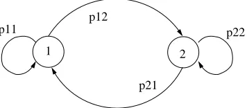
chain process. For example, consider the two state discrete-time Markov
chain (DTMC) represented by Figure 3.2.
1 2
p22 p11
p21 p12
Figure 3.2: DTMC transition diagram
We can represent the same Markov chain by its 2 x 2 transition probability
matrix P:
P =
p11 p12 p21 p22
where the rows of P sum to 1.
let-ters for vectors, and we refer to the size of a matrix as n x n, where n is the
number of states in the Markov chain model. For the individual elements of
a vector we use subscripts on lowercase letters. For example,x2 is the second element in the vector x= [x1, x2, x3, . . . , xn].
For successive vectors resulting from iteration we use a superscripted
index enclosed in parentheses, such as x(1), x(2), x(3), . . .. Lastly, we generally use Greek letters for important scalar quantities—the exception to this is the
Greek letter π which we use to represent the stationary solution vector.
3.3
Definitions and Terminology
For what follows we need definitions of several Markov chain terms. Each of
these terms refers to a property of Markov chains that have an impact on the
selection of a solution method when computing the stationary distribution.
A Markov chain isirreducible if every state in the chain is reachable from
every other state in the chain. Markov chains that do not have this property
are called reducible. This property is easily seen in a transition diagram.
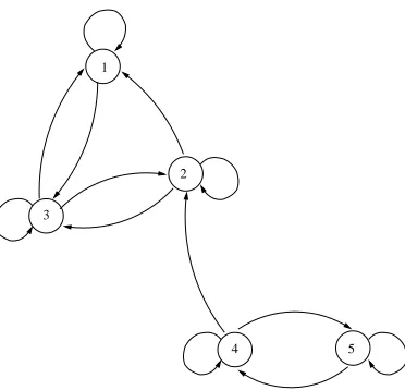
For example, in Figure 3.3 we see a reducible Markov chain because states 4
and 5 are not reachable from states {1,2,3}. If states 4 and 5 were deleted,
along with the associated arcs, then the remaining states {1,2,3} would
form an irreducible transition diagram for a Markov chain. Alternatively, if
the {4} → {2} arc is deleted then we are left with two distinct, irreducible
5 4
3 1
2
Figure 3.3: A reducible Markov chain
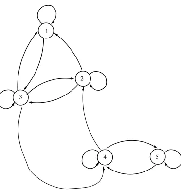
A Markov chain is said to be nearly completely decomposable if certain
transition probabilities are (relatively) small enough so that the chain can
almost be broken into two or more separate Markov chains. For short, we
use the acronym NCD. For example, consider Figure 3.4. Imagine that the
thin arcs {3} → {4} and {4} → {2} have considerably less magnitude than
the heavy arcs. Based on our previous example, we see that this Markov
chain is irreducible; however, if the two thin arcs are deleted we have two
structures that qualify as stand-alone Markov chains. Because of this, we say
that the Markov chain in Figure 3.4 defined by states {1,2,3,4,5} is NCD.
The property of being NCD is also evident in the matrix representation of
this Markov chain. Suppose that the transition diagram in Figure 3.4 has
transition probabilities as shown in matrix (3.4). The matrix (3.4) shows that
most of the probability is in the two diagonal blocks and very little probability
3 1
2
5 4
Figure 3.4: An NCD Markov chain
into two separate Markov chains matrices.
P =
.8501 .0 .1499 .0 .0
.1 .65090 .249 .0 .0
.1 .8 .09970 .0003 .0
.0 .0004 .0 .7 .2995
.0 .0 .0 .3995 .6004
(3.4) .
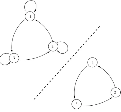
The final property to consider isperiodicity. The directed graph of every
irreducible Markov chain contains at least one elementary cycle. An
elemen-tary cycle is a path from state i back to stateiwhere no intermediate states
are repeated. The length of an elementary cycle is the number of steps
re-quired to return to the starting state. Some states have self-loops which are
elementary cycles of length 1. Most Markov chains have several elementary
cycles in a given Markov chain. Then the periodicity of the Markov chain is
defined as
p= gcd{cl1, cl2,· · ·, clk} (3.5)
where gcd≡greatest common divisor. For example, in Figure 3.5, the upper
figure has elementary cycles of length 1 and 3—so the period is 1. In the
lower graph, all elementary cycles are of length 3—here the period is 3. A
matrix is termed aperiodic if p= 1.
3 1
2
3 1
2
Figure 3.5: An example of periodicity
Kulkarni [23] describes five aspects of a stochastic process and we discuss
them here as a way of framing the focus of this dissertation:
• Characterization. We focus on stochastic processes that have the Markov
property. Markov chains have additional classifications based on their
• Transient behavior. This is the distribution of the process at a
par-ticular time, t or n, and the observation of how the process changes
through time.
• Limiting behavior. This is the behavior of the process as time → ∞
and is the main focus of our current research. Under certain structural
conditions, the limiting behavior of a Markov chain is interpreted as
the probability of finding the process in a particular state; under other
conditions its interpretation is the fraction of time the process spends
in each state.
• First passage times. This is the examination of when the process first
enters a particular state or set of states.
• Costs and Rewards. This aspect considers the costs and rewards
gen-erated by the process based on which states are visited and how long
the process is in a particular state.
In the case of a continuous-time Markov chain (CTMC) the transitions from
one state to another are distributed exponentially and the matrix
represent-ing the Markov chain is a matrix of transition rates. TheMarkov property is
still present and is described mathematically as
P r{X(tn+1) = j|X(t0) = i0, X(t1) =i1, . . . , X(tn) = in}
for time sequencet0, t1, . . . , tn, tn+1and possible statesi0, i1, . . . , in−1, in, j. In a manner analogous to the DTMC, the limiting distribution of an irreducible
CTMC is the solution π to
πQ= 0, X
i
πi = 1, π ≥0. (3.7)
In this case, the rows of Q sum to zero and qij is an element of Q. The
element qij is the rate of transition from state i toj. The diagonal elements
are defined by
qii=−X
i6=j
qij.
The system in (3.7) is assured of a non-zero solution vector π because the
matrix Qis singular with rank (n−1) [37]. We can rewrite system (3.7) as
QTπT = 0.
For a DTMC we can also describe the problem of obtaining π as the
solution to a homogeneous linear system. We are able to do this because of
the following equalities that allow us to express the matrix P in terms ofQ,
and vice versa:
Q=I−P, and P = ∆t Q+I, (3.8)
where I is the identity matrix and
∆t = 1
For a DTMC we rewrite equation (3.1) as
πP = π
πP −π = 0
π−πP = 0
π(I −P) = 0, (3.9)
and letting Q = I −P, we obtain πQ = 0, which is identical to (3.7). In
both cases, we see that the solution vector π can be obtained by solving the
linear system
QTπT = 0, X
i
πi = 1, π ≥0. (3.10)
The solution vector π to the systems (3.1) and (3.7) is also called the
sta-tionary probability vector.
When the Markov chain is finite, irreducible, and aperiodic then the
el-ement πj from the vector π is interpreted as both the probability of finding
the process in statej and the long-run proportion of time the process spends
in state j. When the Markov chain is finite, irreducible, and periodic, the
el-ement πj from the vector π is interpreted as the long-run proportion of time
the process spend in state j. In both cases, the unique solution to (3.10)
provides the vector π. The reader is invited to see references [37, 44, 33] for
Chapter 4
Solution Methods
Solution methods for obtaining the vector π include direct, iterative,
projec-tion, anddecompositional methods [5, 16, 23, 30, 37, 38], as well as various
ap-proximation and bounding techniques such as those described by Semal [36].
Direct methods always terminate in a finite number of operations and this
number can be accurately computed before starting the algorithm.
Con-versely, iterative methods use a convergence-based stopping criteria and the
exact number of operations (or iterations) is unknown until the algorithm is
applied to the matrix at hand. In general, iterative methods begin with an
initial solution and at each step update the current solution to obtain the
next solution approximation.
Projection methods do have an iterative aspect to them but instead of
up-dating the solution vector at each iteration, projection methods repeatedly
from the vectors within the current subspace. The result is an improving
se-quence of solution vectors{xk}that result in convergence to the solution [38].
Decompositional methods are appropriate for use on Markov chain
ma-trices that are NCD, or nearly completely decomposable. Since the matrix is
nearly decomposable, a tempting idea is to divide the matrix into its largest
parts, find their individual solutions, and then somehow combine the
indi-vidual solutions to obtain the overall solution. This is the concept of divide
and conquer [37].
Each of the four solution categories are considered in more detail later
when we discuss their implementation and application.
4.1
Direct Methods
Gaussian elimination is the oldest method for solving a linear system.
Ma-trices and determinants were seriously studied as long ago as the second
century BC and in the early 1800s Gauss proposed the solution method we
know today as Gaussian elimination [3]. When applied to a discrete time
Markov chain, the solution vector π that we seek is the solution to the linear
system
πP =π, X
i
πi = 1, π ≥0 (4.1)
whereP is the transition probability matrix of the Markov chain. The system
of (4.1) can be rewritten using Q = I −P to obtain QTπT = 0. Now we
singular coefficient matrix [30].
For reasonable sized systems, Gaussian elimination is efficient and
ac-curate. Through elementary row operations the coefficient matrix is
trans-formed into an upper triangular system and then the solution is obtained
through back-substitution. Because the matrixQT has rank (n−1), the
ele-mentary row operations end with the last row of the reduced matrix having
all zero elements. This allows us to assign an arbitrary value to the πn
ele-ment and proceed with the back-substitution to obtain a solution. Recalling
the requirement for Piπi = 1, we can normalize the result and obtain the
desired solution vector π.
For large problems, depending on the initial structure of the matrix, a
direct method can cause fill-in as the computations progress. Fill-in is the
replacement of zero elements with non-zero elements. For a large matrix, the
creation of new, non-zero elements can create a memory shortage. The fill-in
is limited when the matrix has a banded structure with most of the non-zero
elements close to the main diagonal. Thus direct methods are appropriate
for small matrices or matrices where excessive fill-in will not occur.
4.2
Iterative Methods
Iterative methods are generally preferred to direct methods unless the matrix
has a special structure that can be exploited [38]. Iterative methods have the
computations. Once the matrix is stored in a compact form no fill-in or
changes are made to the matrix [37]. Iterative methods can also be faster
than direct methods.
The power method is the simplest of the iterative methods for obtaining
the stationary vectorπand is one of the keys to understanding the Successive
Over-Relaxation (SOR) method that we use in this research.
4.2.1
The Power Method
The stationary distribution vectorπ of an irreducible Markov chain satisfies
the matrix-vector equation π =πP, where π is the left-hand eigenvector of
P corresponding to the unit eigenvalue. Again,P is the matrix of transition
probabilities. If P is also aperiodic, then π can be obtained through an
iterative scheme as shown in 4.2. Recall that π(i) is the approximation of the vector π at iteration i.
π(1) = π(0)P
π(2) = π(1)P = (π(0)P)P =π(0)P2
π(3) = π(2)P =π(0)P3
.. . ... ...
Under the previously mentioned conditions on P,
lim
k→∞π
(k) =π.
Letting x=πT, an iteration scheme based on the above can be expressed as
x(k+1) =PTx(k). (4.3)
This method for obtaining π is called the power method. If the Markov
chain is aperiodic and irreducible, then the iteration matrix has a simple
unit eigenvalue (λ1 = 1) and the power method converges; however, the rate of convergence depends on the sub-dominant (second largest) eigenvalue, λ2, and the ratio
|λ2|
|λ1|. (4.4)
The smaller the ratio, the faster the convergence of the power method. If
|λ2| ≈ 1 then the power method has little practical value because the
con-vergence is too slow.
Initial Iteration Vector
The simplest initial vector to use with an (nxn) Markov chain matrix system
Stopping Criterion
As noted at the start of this section, we hope the chosen iterative method
produces a converging sequence (4.5) of iterates (vectors) that end up being
acceptably close to the exact solution for our system of equations. To make
this scheme complete, we must consider appropriate stopping criteria. For
general linear systems Ax = b, stopping criteria usually involve either the residual, defined as r(k) =Ax(k)−b, or some other suitable measurement of the progress being made towards the solution. If the residual is used, then
the algorithm can be stopped when
kr(k)k ≤²,
where ² is a user-defined tolerance. See Barrett [5] for more details. If
progress toward a solution is used as the stopping criterion, then the
algo-rithm can be halted when continued iterations yield little or no additional
improvement in the solution. This is measured by the norm of thedifference
of successive iteration vectors:
kx(k)−x(k−1)k ≤².
This stopping criterion works well for iterative methods that exhibit at least
somewhat monotone convergence, such as the Jacobi, Gauss-Seidel, and SOR
4.2.2
Additional Iterative Methods
Other iterative methods for determining the stationary distribution of a
Markov chain are derived from iterative methods for the solution of
lin-ear systems Ax = b. An iterative method for solving Ax = b constructs a
sequence of approximate solution vectors
x(0), x(1), x(2),· · ·, x(i),· · · (4.5)
with the goal of quickly converging to the solution (within an acceptable
tolerance level). Here x(0) is a initial vector used to start the algorithm. If the system arises from a Markov chain, then x(0) is a probability vector that must satisfy the normalization constraint Pixi = 1. The iteration scheme
takes the form
x(k) =Bx(k−1)+c, (4.6)
where the matrix B and the vector c are both time-invariant. The
itera-tion formula (4.6) arises from a conveniently1 chosen splitting of the original coefficient matrix A. For example, let A=M −N, then
Ax = b
(M −N)x = b
M x−N x = b
M x = N x+b
x = M−1N x+M−1b. (4.7)
Letting B =M−1N and c=M−1b, we can see that equation (4.7) is equiv-alent to equation (4.6).
In the particular case of a Markov chain, the stationary distribution is the
solution to the homogeneous system 0 = πQ or QTπT = 0. Letting x = πT
we obtain
QTx= 0. (4.8)
Here Q is the (n x n) infinitesimal generator matrix of the Markov chain.
Since P has a unit eigenvalue, the matrixQ= (I−P) has a zero eigenvalue,
and equation (4.8) has a non-trivial solution [37]. Since the right-hand side
of equation (4.8) is zero the iteration scheme of (4.6) becomes
x(k+1)=Bx(k). (4.9)
At convergence, x=Bx and x is the right-hand eigenvector of the iteration
matrixBcorresponding to the unit eigenvalue. Note that equations (4.3) and
(4.9) are of identical form. So we see that the iterative solution to QTx =
0 via a splitting technique is the same as the power method applied to an
appropriately chosen iteration matrix B. The same ratio of the dominant
and sub-dominant eigenvalues of the iteration matrix shown in (4.4) controls
We next examine three iterative solution methods that successively build
on each other and each use a splitting technique: the Jacobi, Gauss-Seidel,
and the Successive Overrelaxation (SOR). We then discuss in detail a
modi-fication of the SOR method that makes it easier for novice users to employ.
Jacobi Method
The method of Jacobi considers the matrix splittingQT =D−(L+U), where
D, L, and U are, respectively, the diagonal, lower, and upper structures of
the coefficient matrix. Then
QTx = 0
[D−(L+U)]x = 0
Dx = (L+U)x
x(k+1) = D−1(L+U)x(k). (4.10) Equation 4.10 is then a power iteration with iteration matrixBJ =D−1(L+
U).
Gauss-Seidel Method
When the method of Jacobi is executed in an algorithm, the elements,xi, of
the next approximate solution vector are computed in sequence as the
newly computed elements of the next solution vector constitute the most
recent information about the solution vector. Accordingly, in Gauss-Seidel,
the most recently computed elements x1, x2,· · ·, xi are used for the matrix-vector product that yields the xi+1 element. This amounts to a splitting of
the coefficient matrix as QT = (D−L)−U. Then
QTx = 0
[(D−L)−U]x = 0
(D−L)x−U x = 0
(D−L)x = U x
x(k+1) = (D−L)−1U x(k). (4.11) Equation 4.11 is then a power iteration with iteration matrix BGS = (D−
L)−1U.
SOR Method
The method of Successive Overrelaxation (SOR) is a modification of the
Gauss-Seidel method. SOR iterates are computed by taking a weighted linear
combination of the previously computed iterate and the current Gauss-Seidel
iterate for each component:
where the ¯xdenotes the current Gauss-Seidel iterate and ω is the relaxation
parameter [5]. Note that when ω = 1, then SOR iteration is identical to the
Gauss-Seidel method. The SOR method generally follows the same splitting
approach that was used for Jacobi and Gauss-Seidel. For SOR, the splitting
can be observed as QT = M − N where M = ω−1[D − ωL] and N =
ω−1[(1−ω)D+ωU] [37]. Then
x(k+1) = (D−ωL)−1[(1−ω)D+ωU]x(k) (4.13) and equation (4.13) is a power iteration with iteration matrix BSOR = (D−
ωL)−1[(1−ω)D+ωU].
The relaxation parameter ω is valid for 0 < ω <2, and it can be shown
that SOR fails to converge if ω ≤ 0 or ω ≥ 2 [30]. The optimal choice,
ωopt, for the value of ω is one that accelerates convergence by decreasing the
value of the sub-dominant eigenvalue more than any other ω value. This, in
turn, decreases the ratio (4.4) and accelerates the convergence of the power
iterations.
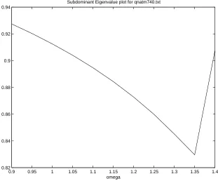
As an example, we show Figure 4.1, which is a plot of the subdominant
eigenvalue of the SOR iteration matrix as a function of ω for the matrix
qnatm740.2
This plot was produced by creating amatlab code loop that repeatedly
forms the SOR iteration matrix and then solves for the three greatest (in
0.9 0.95 1 1.05 1.1 1.15 1.2 1.25 1.3 1.35 1.4 0.82
0.84 0.86 0.88 0.9 0.92 0.94
Subdominant Eigenvalue plot for qnatm740.txt
omega
Figure 4.1: Subdominant eigenvalue plot
magnitude) eigenvalues. The subdominant eigenvalue is then plotted. For
relatively small matrices this can be done in a few minutes but for large
matrices it can be impractical—so it is clear that making plots such as these
it not an efficient means of selecting an ω value for the SOR algorithm.
However, plots like these are helpful in testing an adaptive SOR algorithm.
By adaptive we mean an algorithm that chooses and adaptively changes the
value of ω as the algorithm progresses.
In only a few special cases can the value ofωopt be determined in advance
(see [30] for a discussion). In general, the value of omega is determined
value of ω as the SOR iterations proceed. While simple in concept, the
actual implementation of an adaptive SOR algorithm is somewhat complex.
Many authors who describe the SOR method do not discuss adaptive schemes
in detail, if at all.
A trial and error implementation of SOR begins when the user selects a
value for the relaxation parameter (ω) and starts the SOR algorithm. The
user observes the results and then repeats the cycle, picking a new ω, until
convergence is obtained in a reasonable number of iterations. This is neither
a satisfactory nor systematic approach since for some choices of ω the SOR
iteration probably fails to converge. Additionally, this approach fails to take
advantage of information that is available in the Markov chain matrix.
Conversely, an adaptive SOR procedure does not require the user to
choose a value for omega. Instead the program assumes a default starting
value of omega and begins iterations. The value of omega is then adaptively
changed to obtain convergence of the iterations.
In this research we experimented with several approaches for adaptively
choosing an ω value. These included using a Golden Section search [7] and
the method of Merrall [24].
The Golden Section search is an efficient one-dimensional, non-gradient
search for locating the minimum of a function within a bounded interval. It
is based on the ancient intervals of g and 1−g, where
g = −1 +
√
and g is used for dividing a line or a solid object [7]. The search proceeds
by evaluating the function initially at 2 points and then discarding the point
(and interval) which is furthest from the minimum of the function.
Subse-quent iterations only need one functional evaluation. This is an appealing
idea for finding the value of ω that gives us the best SOR iteration matrix
but we do not know the function for the curve in Figure 4.1; this would seem
to prohibit the use of a Golden Section Search. To overcome this difficultly
we used a convergence ratio test in place of a functional evaluation.
Unfor-tunately, the Golden Section method was not sensitive enough to adaptively
adjust ω. Figure 4.2 shows the Golden Section adjustment for thekanban55
matrix. For this matrix, ωopt ≈ 1.0 and the Golden Section adjustment
widely oscillates and then stabilizes far from the optimum ω value.
Merrall’s method attempts to locate the optimum ω by starting with
ω = 0.5 and adjusting the value ever higher while a convergence ratio is used
to sense the characteristic cusp that reveals the optimum value of ω (see
Figure 4.1). This type of cusp is present for every SOR iteration matrix.
Merrall makes the assumption that the cusp (and his convergence ratio) are
approximately polynomial near the minimum. He tests for changes in the
convergence ratio and then uses a Newton polynomial interpolation on the
last three values of the convergence ratio. We had some success with Merrall’s
approach but found it tricky to sense the cusp. We also disliked the brute
0 2 4 6 8 10 12 14 0.5
0.6 0.7 0.8 0.9 1 1.1 1.2 1.3
iterations
Omega
Figure 4.2: Golden Section adaptive ω adjustment forkanban55 matrix
expert; that is, start withω = 1.0 and adjust up or down based on how the
SOR algorithm behaves.
Our implementation is based on a method demonstrated by Barth [6]
whereω0 = 1.0 and then is adjusted up or down depending on observation of a convergence ratio; however, based on experimentation we chose a convergence
ratio different than that presented in his paper.
In addition to the convergence test contained within the basic SOR
al-gorithm, a convergence ratio is defined to indicate the effect of the changes
inω. The∞-norm is computed on the difference between successive iterates
value of ω and then successive iterates are used in a ratio [4].
We define a convergence ratio as
αk= kx
k−xk−20 k
∞
kxk−20−xk−40k∞. (4.14)
Each two consecutive values ofαare compared. We favor values ofαthat are
progressively getting smaller because this indicates convergence. We continue
to increment the value of ω according the rule
ωk+1 =ωk+ ∆k (4.15)
where ∆0 = 0.1 at the start of the algorithm. Since the majority of systems respond best toover-relaxation we start our adaptive procedure by assuming
that ω increases fromω = 1.0. If the most recent value ofα is greater than
the previous value then we make the assumption that the value of ω needs
adjustment in the opposite direction. We set
∆k+1 =−∆k 2
and again increment ω according to (4.15).
Once begun, the adaptive process continues until one of three events occurs:
1. The SOR algorithm converges for some value ofω.
0 100 200 300 400 500 600 700 800 0.65
0.7 0.75 0.8 0.85 0.9 0.95 1 1.05 1.1
Iterations
Omega
Figure 4.3: Convergence ratio adaptive ω adjustment for kanban55 matrix
then set toω = 1.85 and the SOR continues to its natural completion.
3. The omega value is decremented toω ≤0.50. If this occurs then omega
is then set toω = 0.50 and the SOR continues to its natural completion.
As an example, again consider Figure 4.3 which shows the adaptive
ad-justment of ω for the matrix kanban55. After starting at 1.0, the value of
ω is adjusted every 60 iterations and finally is stabilized at ω = 0.96875
until convergence occurs. The final ω is very close to ωopt ≈ 1.0. Compare
Figure 4.3 to Figure 4.2 which shows the use of a Golden Section search.
The Golden Section search oscillates widely and does not stabilize near the
While testing various Markov chain models for this research, we
discov-ered a case where the adaptive procedure adjusted the ω value too far. This
caused the algorithm to nearly converge and then quickly veer away from
con-vergence to failure. This behavior was only observed in the ridler model
(see Section 8.1). To counteract this effect, we added code that monitors the
convergence criteria and catches this type of behavior. When detected, the
ω value is reset backtwo steps and stabilized. This mechanism corrected the
problem and allowed convergence for this model.
In summary, we had the best results when we started at ω = 1.0 and
adaptively adjusted based on a convergence ratio measured at spaced
inter-vals. Hovland and Heath [19] report some success using a derivative-based
method to adjust ω. We did not experiment with their methods but we did
observe the same phenomenon: we found that some models return faster
SOR times with adaptiveω adjustment than with iterations where the
relax-ation parameter is fixed atωopt. An extensive literature search did not reveal
any explanation for this behavior. On the surface, this behavior does not
make sense because the value of ω is responsible for altering the eigenvalue
ratio given in (4.4). Areas that could be investigated include the structure
of the iteration matrix and the fact that in the adaptive SOR algorithm the
Block Versions of Jacobi, GS and SOR
Each of the previously described point iterative algorithms has a block
ver-sion. Block iterative methods are sometimes useful when the states of a
matrix can be partitioned (and permuted) into meaningful groups, or blocks.
One example where this occurs is in matrices that are Nearly Completely
Decomposable, or NCD. The following 8×8 matrix taken from [37] is NCD
with three distinct diagonal blocks that are nearly decomposable into three
distinct Markov chains.
P =
.85 .0 .149 .0009 .0 .00005 .0 .00005
.1 .65000 .249 .0 .0009 .00005 .0 .00005
.1 .8 .09960 .0003 .0 .0 .0001 .0
.0 .0004 .0 .7 .2995 .0 .0001 .0
.0005 .0 .0004 .399 .6 .0001 .0 0
.0 .00005 .0 .0 .00005 .6 .2499 .15
.00003 .0 .00003 0.00004 .0 .1 .8 .0999
.0 .00005 .0 .0 .00005 .1999 .25 .55
.
From equation (4.8) we can envision blocks of states where
QT11 QT12 · · · QT1N QT21 QT22 · · · QT2N
..
. ... . .. ...
QTN1 QTN2 · · · QTNN
x1 x2 .. . xN
The block Jacobi iterative method splits QT into
QT =DN −(LN +UN),
where DN is ablock diagonal matrix, LN is alower block triangular matrix,
and UN is an upper block triangular matrix. Each Jacobi iteration has the
form
DNx(k+1) = (LN +UN)x(k).
Letting ZN = (LN +UN)x(k), we see that for every Jacobi iteration we must solve N systems of equations:
DNx(k+1) =ZN.
The Jacobi iterations are called outer iterations. The N inner systems of
equations can be solved by any appropriate method. If the inner system is
small enough then Gaussian elimination may be appropriate; if not, then
an iterative method such as Gauss-Seidel can be used. We expect that the
additional effort per iteration to solve the N systems is rewarded by fewer
4.3
Projection Methods
Projection methods repeatedly create small-dimension subspaces and seek
the best approximate solution from the vectors within the current subspace.
The result is an improving sequence of vectors {x(k)} that converge to the solution. Here we focus on Krylov subspace projection methods. Common
Krylov methods include the generalized minimum residual (GMRES),
con-jugate gradient (CG), and bi-concon-jugate gradient stabilized (BiCGSTAB).
Krylov methods are based on the observation that an approximate
solu-tion vector, x, to an (n×n) system of equations, Ax=b, lies in a subspace
whose dimension is generally smaller than the order of A (m ¿ n). If m
is small, then a solution method based on Krylov subspaces might quickly
converge to the solution. See [20] for more details.
Starting with an initial solution guess, x(0), a Krylov projection method finds the best approximation, x(k) = x(0)+z, to the exact solution. It does this by selecting a vector z from vectors in the Krylov subspace Kk where
Kk(A, c)≡span{c, Ac, A2c, . . . , Ak−1c} (4.16)
for some vector c. When the solution sequence, {x(k)}, is designed to build a basis for the subspace, Kk, the projection method terminates in at most n
iterations (since there can be no more than n linearly independent vectors in
a subspace of dimension n) [37, 20].
a Krylov subspace, it helps to consider that our solution is x = A−1b. Let
m be the degree of the minimal polynomial of A, ψm(A) = 0. Then as a
concrete example, imagine a matrix A with m = 3. Then
0 = ψ3(A)
0 = α0I+α1A+α2A2+α3A3
α0I = −(α1A+α2A2+α3A3)
I = − 1
α0(α1A+α2A
2+α 3A3)
A−1I = − 1
α0(α1A
−1A+α
2A−1A2+α3A−1A3)
A−1 = − 1
α0(α1+α2A+α3A
2).
Recalling that x=A−1b, then
x=A−1b=− 1
α0(α1b+α2Ab+α3A
2b)
and we can see that x∈ K3(A, b).
Conjugate Gradient Methods
In this section our goal is to describe the use of the bi-conjugate gradient
stabilized (BiCGSTAB) algorithm as a method for finding the stationary
dis-tribution of a Markov chain by solving QTπT = 0. The BiCGSTAB method
gradi-ent (CG), Bi-conjugate gradigradi-ent (BiCG), and the conjugate gradigradi-ent squared
(CGS) methods for solving Ax=b. To understand BiCGSTAB we first need
to review the underpinnings of its related methods.
If the matrix A is symmetric and positive definite, then the solution to
the system Ax=b is equivalent to minimizing the quadratic function
F(y) = 1 2y
TAy−yTb. (4.17)
The minimum can be found using the gradient or steepest descent method.
Starting with an initial approximation, x(0), the approach consists of two parts in each iteration: (i) choose a direction, d, and (ii) choose how far
to proceed in that direction (step parameter, α, chosen to minimize
equa-tion 4.17). For a symmetric, positive definite matrix A, let d =r =b−Ax.
Then the steepest descent method is represented by
Do until convergence:
• Compute scalar α
• Updatex=x+αr
• Updater=b−Ax
At each iteration the value of α is calculated as
αk = r
(k)T r(k) r(k)TAr(k).
This value of α minimizes F(x+αr) which is equation (4.17) evaluated at