An Advanced Algorithm for Construction of Integral Transport Matrix Method Operators Using Accumulation of Single Cell Coupling Factors.

(1)

ABSTRACT

POWELL, BRIAN PAUL. An Advanced Algorithm for Construction of Integral Transport Matrix Method Operators Using Accumulation of Single Cell Coupling Factors. (Under the direction of Yousry Y. Azmy.)

The Integral Transport Matrix Method (ITMM) has been shown to be an effective method

for solving the neutron transport equation in large domains on massively parallel architectures. In the limit of very large number of processors, the speed of the algorithm, and its suitability for

unstructured meshes, i.e. other than an ordered Cartesian grid, is limited by the construction

of four matrix operators required for obtaining the solution in each sub-domain. The existing algorithm used for construction of these matrix operators, termed the differential mesh sweep,

is computationally expensive and was developed for a structured grid. This work proposes the

use of a new algorithm for construction of these operators based on the construction of a single, fundamental matrix representing the transport of a particle along every possible path

through-out the sub-domain mesh. Each of the operators is constructed by multiplying an element of

this fundamental matrix by two factors dependent only upon the operator being constructed and on properties of the emitting and incident cells. The ITMM matrix operator construction

time for the new algorithm is demonstrated to be shorter than the existing algorithm in all

tested cases with both isotropic and anisotropic scattering considered. While also being a more efficient algorithm on a structured Cartesian grid, the new algorithm is promising in its

geo-metric robustness and potential for being applied to an unstructured mesh, with the ultimate

(2)

(3)

An Advanced Algorithm for Construction of Integral Transport Matrix Method Operators Using Accumulation of Single Cell Coupling Factors

by

Brian Paul Powell

A thesis submitted to the Graduate Faculty of North Carolina State University

in partial fulfillment of the requirements for the Degree of

Master of Science

Nuclear Engineering

Raleigh, North Carolina

2013

APPROVED BY:

Dmitriy Y. Anistratov Robert E. White

(4)

DEDICATION

(5)

BIOGRAPHY

The author graduated from the United States Military Academy at West Point in May, 2006 with a B.S. in Nuclear Engineering. He then served as an active duty U.S. Army Officer from

2006 to 2011 with deployments to both Iraq and Afghanistan. In 2011, Brian returned to academia to pursue graduate studies in Nuclear Engineering, specifically in the field of

Compu-tational Neutron Transport Theory under the direction of Professor Yousry Y. Azmy. In 2012,

(6)

ACKNOWLEDGEMENTS

The Department of Energy Computational Science Graduate Fellowship (DOE CSGF) and the Department of Energy Nuclear Energy University Program (DOE NEUP) both supported this

(7)

TABLE OF CONTENTS

List of Tables . . . vi

List of Figures . . . vii

Chapter 1 Introduction . . . 1

Chapter 2 Review of Literature . . . 3

2.1 Discretization of the Transport Equation . . . 3

2.2 Parallel Domain Decomposition of the Transport Equation . . . 5

2.3 Response Matrix Methods . . . 6

2.4 The Integral Transport Matrix Method . . . 8

Chapter 3 The Integral Transport Matrix Method . . . 10

3.1 Consideration of Anisotropic Scattering . . . 14

3.2 The Differential Mesh Sweep (DMS) Algorithm . . . 16

Chapter 4 The Fundamental Matrix Method Algorithm . . . 20

4.1 Example Construction of Elements of F for a 3 x 3 Cell Domain . . . 30

Chapter 5 Performance Model and Timing Results . . . 51

5.1 Performance Model . . . 51

5.2 Timing Results . . . 53

5.3 Memory Requirements . . . 57

Chapter 6 Conclusions. . . 61

(8)

LIST OF TABLES

Table 3.1 Matrix Operator Definitions . . . 14

Table 4.1 Emergent and Incident Multipliers of F_n₍_i,j,k₎₍_i0_,j0_,k0₎_,di,df for Construction of ITMM Operators . . . 26

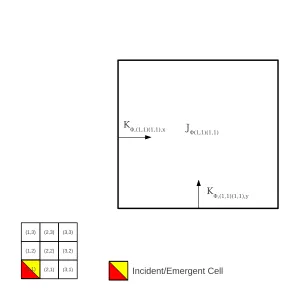
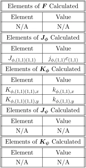
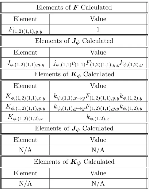
Table 4.2 Values of Nonzero Elements of F, Jφ, Kφ, Jψ, and Kψ Resulting from an Angular Flux Incident on a Face of Cell (1,1) for an Ordinate in the Primary Octant . . . 33

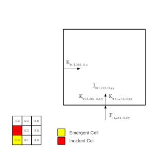
Table 4.3 Values of Nonzero Elements ofF,Jφ,Kφ,Jψ, andKψResulting from an Angular Flux Incident on a Face of Cell (1,2) and Emergent from a Face of Cell (1,1) for an Ordinate in the Primary Octant . . . 35

Table 5.1 Matrix Operator Construction Time (s) for L=0 (isotropic) . . . 53

Table 5.2 Matrix Operator Construction Time (s) for L=1 . . . 54

Table 5.3 Matrix Operator Construction Time (s) for L=3 . . . 54

Table 5.4 Least Squares Fit Constant Values for Equation 5.6 . . . 55

Table 5.5 Matrix Operator Memory Requirements for L=0 . . . 58

(9)

LIST OF FIGURES

Figure 4.1 Two Dimensional Representation of F_n₍_i,j₎₍_i0_,j0₎_,y,x for an Ordinate in the

Primary Octant . . . 22 Figure 4.2 Two Dimensional Representation of Fn(i,j)(i0_,j0₎_,y,y for an Ordinate in the

Primary Octant . . . 23 Figure 4.3 Two Dimensional Representation ofF_n₍_i,j₎₍_i0_,j0₎_,x,x for an Ordinate in the

Primary Octant . . . 24 Figure 4.4 Two Dimensional Representation of Fn(i,j)(i0_,j0₎_,x,y for an Ordinate in the

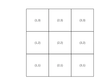
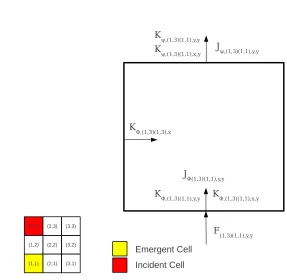
Primary Octant . . . 25 Figure 4.5 3 x 3 Cell Domain with Numbered Cells . . . 30 Figure 4.6 Construction Basis of All Four ITMM Operators Resulting from an

An-gular Flux Incident on a Face of Cell (1,1) for an Ordinate in the Primary Octant . . . 32 Figure 4.7 Construction Basis of All Four ITMM Operators Resulting from an

An-gular Flux Incident on a Face of Cell (1,2) and Emergent from a Face of Cell (1,1) for an Ordinate in the Primary Octant . . . 34 Figure 4.8 Construction Basis of All Four ITMM Operators Resulting from an

An-gular Flux Incident on a Face of Cell (3,3) and Emergent from a Face of Cell (1,1) for an Ordinate in the Primary Octant . . . 48

Figure 5.1 Performance Model (lines) and Measured Matrix Operator Construction Times (triangles) for L=0 (isotropic scattering) . . . 55 Figure 5.2 Performance Model (lines) and Measured Matrix Operator Construction

(10)

(11)

Chapter 1

Introduction

The neutron transport equation governs neutron movement through a medium over time at various energies and directions. The neutron transport equation is [1]

1

v ∂ ∂tψ(~r,

ˆ

Ω, E, t) + ˆΩ·5ψ~ (~r,Ωˆ, E, t) +σ(~r, E)ψ(~r,Ωˆ, E, t) =σs(~r, E)φ(~r, E, t) +q(~r,Ωˆ, E, t) ,

(1.1)

where v is the neutron speed, ψ(~r,Ωˆ, E, t) is the neutron angular flux at position~r, direction of travel ˆΩ , energyE, and timet, σ(~r, E) is the total neutron cross section at position ~r and

energyE,σs(~r, E) is the neutron scattering cross section at position~r and energy E,φ(~r, E, t)

is the neutron scalar flux at position ~r, energy E, and time t, and q(~r,Ωˆ, E, t) is the fixed neutron source at position~r, direction of travel ˆΩ , energy E, and timet.

For the purposes of this work, the neutron transport equation is considered to be time-independent.

The removal of the time variable results in the form of the transport equation considered here,

ˆ

Ω·5ψ~ (~r,Ωˆ, E) +σ(~r, E)ψ(~r,Ωˆ, E) =σs(~r, E)φ(r, E~ ) +q(~r,Ωˆ, E) . (1.2)

This form of the transport equation must be discretized in space, angle, and energy to allow for

a numerical solution. The Integral Transport Matrix Method (ITMM) for solving the neutron transport equation, which is the method examined in detail in this work, makes use of each of

these discretizations.

In the field of computational neutron transport theory, advanced methods for solving the

neu-tron transport equation are needed for solving larger problems on a greater number of proces-sors. Solution algorithms suitable for massively parallel architectures must continue to achieve

speedup as the number of processors is increased. One such method that has shown promise in

this area is the ITMM.

(12)

operators used iteratively in two equations to converge to the solution of the neutron

trans-port equation. This work is motivated by the desire to implement the ITMM on geometries for complicated engineering using unstructured grids. The rise of unstructured tetrahedral mesh

transport methods and codes as a means to a more accurate representation of geometric

con-figurations typical of radiation transport problems requires adaptations of the ITMM for the application of this method to such a mesh.

A complete algorithm for the construction of the four matrix operators on a Cartesian grid has

already been developed. This algorithm, although effective for constructing the matrix opera-tors on a Cartesian grid, is computationally expensive and requires orderly mesh structure to

perform well. As such, the need for a method of constructing the ITMM matrix operators that

is both more computationally efficient and geometrically robust is evident.

The method presented in this work, although confined to three-dimensional Cartesian meshes

at this stage, is promising in that it has demonstrated significantly faster matrix operator

construction times and has the potential to be applied with relative ease to an unstructured tetrahedral mesh. This algorithm derives its efficiency from the fact that all transport of

par-ticles through a mesh, whether originating from a distributed source or an incoming angular flux, follows the same paths from the emergent face of a cell to the incident face of a cell. This

principle allows for the creation of a fundamental matrix for face-to-face transport, off of which

each of the matrix operators required for the ITMM can be constructed. It will therefore be termed the Fundamental Matrix Method (FMM).

In the following chapter, relevant literature will be reviewed. This will be followed by a

deriva-tion of the ITMM. The FMM will then be derived, along with a complete example of the construction of the four ITMM operators for a 3 x 3 cell system in two dimensions. A

per-formance model for the FMM algorithm will then be described, followed by a comparison of

matrix operator construction time results for several different scenarios for both the existing algorithm and the FMM. This will be followed by a comparison of the FMM timing results to

the algorithm performance model. Finally, conclusions will be presented along with thoughts

(13)

Chapter 2

Review of Literature

The Integral Transport Matrix Method (ITMM) of solving the neutron transport equation on multiprocessing platforms is a spatial domain decomposition method and is therefore ideally

ap-plied to a large domain in a massively parallel computational environment. Given that this work

focuses on the construction of the matrix operators needed for the ITMM and not computation of the solution, either in serial or parallel, the review of literature will focus on the development

of the use of matrix operators in solving the neutron transport equation. The ITMM makes

use of angular, spatial, and energy discretization, so a brief review of these methods will be examined as well.

2.1 Discretization of the Transport Equation

Energy discretization methods, generally referred to as multigroup methods, allow for solv-ing the transport equation for neutrons in a specific energy range. This is accomplished by

integrating equation 1.2 over all energies, resulting in [1]

ˆ

Ω·5ψ~ g(~r,Ω) +ˆ σg(~r)ψg(~r,Ω) =ˆ σs,g(~r)φg(r~) +qg(~r,Ω) ,ˆ (2.1)

where the subscript g indicates a specific energy group. Lewis and Miller discuss multigroup

methods in detail [1]. Here, it is sufficient to note that the methods derived in this work solve the transport equation for a single energy group, hence the subscript g will be suppressed.

Angular discretization, as accomplished by the method of discrete ordinates, is a key component

of this work. Discretizing equation 2.1 by angle yields [1]

(µn

∂ ∂x+ηn

∂ ∂y +ξn

∂

(14)

whereµ is the angular cosine in the x-direction, η is the angular cosine in the y-direction, ξ is

the angular cosine in the z-direction, and the subscriptnindicates a discrete angle. The discrete ordinates method has been used in production-level radiation transport codes since the 1960s,

with much of the early development done by Carlson and Lathrop [2]. Significant advances in

discrete ordinates methodology since that time have been described by Larsen and Morel [3]. Lewis and Miller [1] provide a thorough description of a discrete ordinates solution algorithm

in one, two, and three dimensions using the diamond difference spatial differencing method. By

solving the transport equation for the angular flux at several individual angles in quadrature discrete ordinates allows for an accurate approximation to the solution of the transport

equa-tion. However, discrete ordinates algorithms generally require a repetitive and computationally

expensive mesh sweep in order to converge to the solution. In the ITMM formulation, however, only a single mesh sweep was required in single sub-domain, with convergence achieved by

it-erating on the incoming angular flux to each sub-domain [4].

Spatial discretization, also known as spatial differencing, allows for solving the transport equa-tion in a finite domain by separating that domain into multiple nodes, or cells, in each of which

the flux solution can be found and related to neighboring cells. Considering equation 2.2, spatial central differencing of the partial derivatives comprising the streaming operator yields [1]

µn

4xi

(ψn,i+1/2,j,k−ψn,i−1/2,j,k) +

ηn

4yj

(ψn,i,j+1/2,k−ψn,i,j−1/2,k)+

ξn

4z_k(ψn,i,j,k+1/2−ψn,i,j,k−1/2) +σi,j,kψn,i,j,k =σs,i,j,kφi,j,k+qi,j,k . (2.3)

Where i, j, k are the indices of the given cell in the x−, y−, z− direction, respectively. The

subscripti−1/2, j, kindicates the left x-face of celli, j, kand the subscripti+ 1/2, j, kindicates the right x-face of cell i, j, k, with analogous meanings in the y and z directions.

Larsen and Morel [3] describe in detail three methods of spatial discretization used in solving

the transport equation: The characteristic method, the linear discontinuous method, and nodal methods. Any one of these methods form what is called the auxiliary equation, which relates

the incoming and outgoing angular flux in a cell to the angular flux at the cell center. In the

ITMM formulation used in this work, the diamond difference equation is the auxiliary equation of choice. The diamond difference method is the approximation of the angular flux at the cell

center by

ψn,i,j,k =

1

2(ψn,i+1/2,j,k+ψn,i−1/2,j,k) (2.4)

(15)

2.2 Parallel Domain Decomposition of the Transport Equation

The benefits of the ITMM are realized only on multiprocessing platforms. The method is not

competitive in serial mode but is highly competitive in parallel [4] and therefore the application of parallel domain decomposition must be discussed. Domain decomposition can accomplished

through three distinct means: Energy domain decomposition, angular domain decomposition,

and (as in the ITMM formulation) spatial domain decomposition. A hybrid decomposition combining any of these three methods is also possible. Developments in parallel domain

de-composition are also much more recent than discretization methods due to the availability of

parallel computing resources that became widespread starting in the 1980s.

Energy domain decomposition involves solving the transport equation in a sub-domain for

different energy groups, each on a separate processor. The obvious advantage of domain

de-composition by energy is the ability to rapidly solve transport problems involving a large span of energies. As such, energy domain decomposition is particularly applicable to nuclear reactor

core simulation, where neutrons are constantly changing energy through collisions and neutrons

at varying energies have important properties (e.g. thermal neutrons causing fission). Much of the early work in energy domain decomposition was completed by Weinke and Hiromoto [5,6,7].

Despite its applications, energy domain decomposition is the least used of domain

decomposi-tions due to the possibility that the energy groups could be solved out of order, increasing the iterative cost of convergence with increasing number of participating processors[8,9].

Angular domain decomposition is based on the previously described discrete ordinates angular

discretization method, the main difference being that the transport equation can be solved for each ordinate on a separate processor, assuming vacuum boundary conditions on all external

faces of the problem domain. The resulting angular fluxes are then summed in quadrature on

the base processor or in parallel to achieve a solution for the scalar flux, or, if desired, angular moments of the flux. While advantageous in that, in Cartesian geometry, the ordinates do not

need to be solved in any particular order, the disadvantage of angular domain decomposition is

that the decomposition is limited to the number of ordinates, which generally will not exceed several hundred, to a few thousand at the very most. Therefore, this limitation does not allow

for massively parallel implementations of angular domain decomposition schemes. Another

dis-advantage of angular domain decomposition is that the full spatial domain must be replicated on all processors (e.g. large flux arrays), which requires significant memory storage. Fischer and

Azmy [8] detailed a performance model for both angular and spatial domain decomposition

methods in order to determine which method was better applied to a given problem. They concluded that, for a small computational cluster, it is more efficient to discretize by angle and

that the opposite is true as the number of processors is increased. Azmy [9] also described the

(16)

Spatial domain decomposition is the domain decomposition method used by the ITMM. By

separating a domain into multiple smaller sub-domains, each solved on a separate processor, the transport equation can be solved faster. A disadvantage of spatial domain decomposition is

the necessity of a sub-domain to have the solution to the outgoing angular flux in neighboring

domains. Any disadvantage that this causes, however, is outweighed by the ability to decompose the domain into a large number of smaller sub-domains to match the number of available

pro-cessors, assuming (as typical for large applications worthy of massively parallel solution) that

the spatial discretization yields significantly more computational cells than available processors for execution.

Early work in spatial domain decomposition was completed by Yavuz and Larsen [10], who first

attempted a spatial domain decomposition algorithm on one-dimensional and two-dimensional domains. Yavuz and Larsen [11] also developed the Alternating Direction Transport Sweep

(ADTS), which allowed for adjacent sub-domains to receive updated values for the incoming

angular flux. Although their method was able to achieve parallel speedup, it was not designed for massively parallel architectures and is therefore not competitive with the ITMM. A detailed

account of the development of early spatial domain decomposition methods is provided by Azmy [9].

It is important to emphasize one spatial domain decomposition method: The KBA (Koch,

Baker, Alcouffe) algorithm [12,13], also known as the wavefront algorithm, is a method of spa-tial domain decomposition that is used by the current state-of-the-art neutron transport codes

[4]. The KBA algorithm involves the conduct of a sequential mesh sweep on a diagonal

wave-front through the given domain, where the transport equation is solved on a single processor for each sub-domain and the outgoing angular fluxes are used as incoming angular fluxes in

the adjacent sub-domain. It has been shown [13] that the KBA algorithm is effective on

mas-sively parallel architectures. The shortcoming of the KBA algorithm, however, is that, due to the sequential nature of the parallel mesh sweep, some processors must remain dormant. The

ITMM solution algorithm works simultaneously across the entire domain, minimizing unused

processors and therefore is competitive with KBA as a massively parallel spatial domain decom-position method [4]. An important difference to note between the KBA and ITMM algorithms

is that KBA is synchronous and ITMM is asynchronous, resulting in the disadvantage of KBA,

processor idleness, being essentially traded for increasing iterations in the ITMM.

2.3 Response Matrix Methods

(17)

a known quantity (e.g., incoming angular flux at the boundaries) and provide a response (e.g.,

outgoing flux at the boundaries). Each ITMM matrix operator is then essentially a response matrix.

Response matrix methods (RMM) have been developed for use in solving the transport equation,

but with widely varied techniques [1]. A thorough review and derivation of the RMM in addition to applications in nuclear engineering for both transport theory and the diffusion approximation

were provided by Lindahl and Weiss in 1981 [14]. Lindahl and Weiss asserted that the RMM

provides the solution of a transport problem on a large domain by consolidating solutions of smaller sub-domains. They also state that the advantageous characteristic of the RMM is

the ability to consider each sub-domain as a separate problem. This general introduction to the

RMM is remarkably similar to the basis of the ITMM, which breaks a larger domain into smaller sub-domains on a multiprocessing platform, allowing for the consideration of each sub-domain

as a separate problem, where the global solution is obtained by iterating on the angular flux at

the boundaries of the sub-domains. Lindahl and Weiss consider each sub-domain, or node, as they identify it, to be characterized by a response kernel which is, in essence, a probability of

particle interaction inside the node. The response kernel is then more concretely identified as a response matrix which, when multiplied by an incoming angular flux, produces an outgoing

angular flux. The definition of the response matrix is also expanded to include the response of a

sub-domain over several nodes rather than just a single node. Lindahl and Weiss go on to define four distinct response matrices which relate in the incoming current, outgoing current, scalar

flux, and fixed source in the sub-domain. These matrices are used in two equations iterating on

the incoming current to provide a global solution to the transport equation.

The RMM of Lindahl and Weiss bears significant similarity to the ITMM. Both methods,

generally, make use of multiple cell, or node, sub-domains and the four response matrices using

the iterative solution method described in the previous paragraph. The differences lie in the specifics of the method. The RMM uses particle currents, whereas the ITMM is able to make

use of angular flux via the discrete ordinates method and spatial differencing. The response

matrices are also constructed in a very different manner. Lindahl and Weiss use block matrices defining the response of each node individually to construct the larger response matrix. This

construction method leads to computational storage inefficiency by requiring the storage of more

zeros than meaningful data. Contrasting this approach, the ITMM requires the construction of differential matrix operators and, through the use of discrete ordinates, allows for operator

elements to be grouped efficiently and avoids unnecessary storage.

Although response matrix methods exist for several techniques including Monte Carlo, collision probabilities, and finite elements [1], it is the use of discrete ordinates that is the basis for the

(18)

by Hanebutte and Lewis [15], who proposed using a response matrix algorithm to iteratively

solve the transport equation. The same two-equation iteration technique used by Lindahl and Weiss [14] is used to iterate on the incoming angular flux. The main difference between the

two techniques is that Hanebutte and Lewis iterate on the incoming angular flux as opposed to

the incoming current used by Lindahl and Weiss. The discrete ordinates method allows for this difference. The method of Hanebutte and Lewis was also limited to the response of a

single-cell sub-domain and was therefore computationally expensive in an iterative sense. The ITMM

then, is an evolution of the work of both Hanebutte and Lewis and Lindahl and Weiss.

2.4 The Integral Transport Matrix Method

The response matrix algorithm of Hanebutte and Lewis [15] was not further developed until 1997 by Azmy [16], who first proposed a method for using full-domain operators, rather than

single cell operators, to allow for a solution to the transport equation without the need for repetitive mesh sweeps that continue to dominate deterministic method solution algorithms.

Azmy also described the algorithm required to construct the matrix operator that relates the

scalar flux spatial moments in all cells to the fixed source spatial moments. This matrix operator is identified as A in the equation

φv =A(σsφp+S) , (2.5)

whereφv is the scalar flux in the current iteration,φpis the scalar flux in the previous iteration,

σs is the scattering cross section operator (basically a diagonal matrix whose elements are the

cell by cell isotropic scattering cross section), andSis the fixed neutron source. Azmy identified

thatAis essentially an iterative map of the scalar flux. The algorithm to constructAwas based on a mesh sweep using differential relations between the angular flux and scalar flux spatial

moments to create the matrix identified as the iteration Jacobian. An assumption critical to

the development of the ITMM made in this work is that the iterations defined in equation 2.5 are convergent yielding a converged scalar flux solution,φ∞, giving

φ∞= (I−σsA)−1AS . (2.6)

Through this assumption, previous and current iterates of the cell scalar flux converge to the

same value, eliminating a variable and allowing for a solution of the converged cell scalar flux

without iteration based on the matrix operatorAand the fixed neutron sourceS. Azmy’s work is the first thorough description of an algorithm required to create a matrix operator in the

ITMM,A. However, it is limited to the case of vacuum boundary conditions and also does not

(19)

Azmy continued to evolve the method in 1999 [17] by describing a matrix operatorB such that

B= (I−σsA) . (2.7)

Azmy provides a thorough description of the algorithm required to create B, including the

specific values of diagonal and off-diagonal elements of the matrix and also examines

precondi-tioning methods to allow for faster convergence. Although he further developed the algorithm for matrix operator B in this work, he continued to use only vacuum boundary conditions in

his calculations. Rosa, Azmy, and Morel expanded this work in 2009 [18], examining spectral

properties of A and B and further developing the algorithm for the construction of these op-erators on configurations with vacuum boundary conditions. Rosa et al. identified B as the

integral transport matrix.

Zerr provided major developments in the ITMM in 2011 [4] by expanding the method to

in-clude non-vacuum incoming and outgoing angular flux at the boundaries of the sub-domain. In

doing so, he created four matrix operators Jφ, Jψ, Kφ, and Kψ, withJφ related to Azmy’s previously defined operator as

Jφ=AC , (2.8)

where C is the scattering-ratio matrix (a diagonal matrix whose elements are the cell by cell scattering ratios). The use of each of these operators will be described in the following chapter.

Most importantly to this work, Zerr describes the construction algorithm, the Differential Mesh Sweep (DMS), used to create each of the four matrix operators of the ITMM that are necessary

to account for non-trivial incoming angular flux. Zerr also developed a code for parallel

imple-mentation of this algorithm in constructing the operators and iteratively solving the transport equation across sub-domains. The DMS matrix operator construction algorithm is the

moti-vation of this work in that it is desirable, based on the parallel performance demonstrated by

Zerr, for the ITMM to be applied to other geometries. A more geometrically robust and less computationally expensive algorithm for the construction of the four matrix operators would

(20)

Chapter 3

The Integral Transport Matrix

Method

The starting point of the ITMM is the neutron balance equation for a single cell in three

dimensions, which, considering only isotropic scattering, is [1]

εx_n,i,j,kψn,iout,j,k+ε

y

n,i,j,kψn,i,jout,k+ε

z

n,i,j,kψn,i,j,kout+ψn,i,j,k

=ci,j,kφi,j,k+σ−_t,i,j,k1 qi,j,k+εxn,i,j,kψn,iin,j,k+ε

y

n,i,j,kψn,i,jin,k+ε

z

n,i,j,kψn,i,j,kin (3.1)

where,

εx_n,i,j,k = |µn|

σt,i,j,k∆xi

,AFyz. (3.2)

AFyz stands for “analogously for y and z”, and, by the discrete ordinates approximation with

quadrature weightswn, the scalar flux (φ) is related to the angular fluxes (ψ) by the quadrature

sum

φi,j,k=

D

X

n=1

wnψn,i,j,k, (3.3)

where D is the total number of angles. In the above equations, µn is the angular cosine with

respect to the x-axis of the direction of particle travel along thenth discrete ordinate.σt,i,j,k is

the macroscopic total interaction cross section of the material in celli, j, k. ∆xi is the width of

the cell in thexdirection.ci,j,k is the scattering ratio, σs,i,j,k

σt,i,j,k, of the material in celli, j, k, where

σs,i,j,k is the macroscopic scattering cross section in the same cell.qi,j,kis the distributed source

in celli, j, k.ψn,iout,j,kis the angular flux along then

th_{discrete ordinate leaving cell}_{i, j, k} _{out of}

thex =constant face, with analogous definitions for angular flux leaving at the y =constant

and z = constant faces. ψn,iin,j,k is the angular flux traveling along the n

th _{discrete ordinate}

(21)

at they=constantand z=constantfaces. Finally,ψn,i,j,k is the cell-centered angular flux in

celli, j, k of neutrons traveling along thenth discrete ordinate.

The diamond difference relation in all three dimensions is used to establish a closed matrix system of equations for the unknown fluxes on the left hand side of equation 3.1 [1],

ψn,i,j,k =

1

2(ψn,iin,j,k+ψn,iout,j,k),AFyz, (3.4)

resulting in      

1 εz

n,i,j,k ε

y

n,i,j,k εxn,i,j,k

1 −0.5 0 0

1 0 −0.5 0

1 0 0 −0.5

            ψn,i,j,k

ψn,i,j,kout

ψn,i,jout,k

ψn,iout,j,k

      =      

1 εz_n,i,j,k εy_n,i,j,k εx_n,i,j,k

0 0.5 0 0

0 0 0.5 0

0 0 0 0.5

           

ci,j,kφp_i,j,k+σ_t,i,j,k−1 qi,j,k

ψn,i,j,kin

ψn,i,jin,k

ψn,iin,j,k

      . (3.5)

Left multiplying both sides of equation 3.5 by the inverted coefficient matrix from the left hand side yields

      ψn,i,j,k

ψn,i,j,kout

ψn,i,jout,k

ψn,iout,j,k

     

= Γn

     

ci,j,kφp_i,j,k+σ_t,i,j,k−1 qi,j,k

ψn,i,j,kin

ψn,i,jin,k

ψn,iin,j,k

      (3.6) where

Γn =

     

jφ kφ,z kφ,y kφ,x

jψ,z kψ,z→z kψ,y→z kψ,x→z

jψ,y kψ,z→y kψ,y→y kψ,x→y

jψ,x kψ,z→x kψ,y→x kψ,x→x

      (3.7)

The Γ matrix is then a set of coupling factors (named here according to their function,

which will be clarified later) between the distributed (fixed and scattering) source, incoming angular fluxes, and outgoing angular fluxes. Alternative spatial discretization methods

corre-spond to different auxiliary relations, equation 3.4, that yield the same relation, equation 3.5,

(22)

All of the previous equations provide the relationships between the incoming and outgoing

angular flux and the scalar flux for only a single cell. When considering a multi-cell sub-domain, the relationship between the cells is simply an extension of

ψn,i+1in,j,k=ψn,iout,j,k,AFyz (3.8)

Using this relation to extend equation 3.6 to a global system with vacuum boundary condi-tions, the single cell values of φ and q need to be extended to the vectors φand q containing

the values of the scalar flux and fixed source, respectively, in each cell. In a source iteration

scheme with φp as the previous iterate of the scalar flux and φv as the current iterate of the scalar flux using equations 3.6 and 3.3, the system reduces to [4]

φv =A(Cφp+Σ−_t 1q) , (3.9)

where C is the scattering ratio diagonal matrix andΣ−_t 1 is the inverse total cross section diagonal matrix.Ais then a coefficient matrix constructed from elements of Γ which relates the previous scalar flux iterate to the new scalar flux iterate. Azmy [16] definesAas an iterative map

of the scalar flux. Partially differentiating equation 3.9 with respect toφp yields the iteration

Jacobian Matrix,

∂φv

∂φp =AC (3.10)

AC was denoted by Zerr [4] asJφ.

To factorJφ instead ofA from equation 3.9, the second term needs to be altered to

φv =A(Cφp+Σ_t−1ΣsΣ−_s1q) (3.11)

Substituting

C =Σ−_t 1Σs (3.12)

yields

φv =AC(φp+Σ−_s1q) (3.13)

Then, substituting Jφ forAC,

φv =Jφ(φp+Σ−s1q) (3.14)

(23)

φv =φp=φ∞ (3.15) Substituting this relation into equation 3.14 yields

φ∞= (I −Jφ)−1JφΣ−_s1q (3.16)

Removing the constraints of vacuum boundary conditions, as is necessary to apply the

ITMM to a generic sub-domain, requires that the effect of the incoming angular flux on the scalar flux within each cell of the sub-domain be accounted for. To that end, another term is

added to equation 3.14, yielding [4]

φv =Jφ(φp+Σs−1q) +Kφψin (3.17)

where ψin is a vector containing all incoming angular fluxes to the sub-domain and Kφ is a matrix operator constructed from the elements of Γ which defines the effect of the incoming

angular flux on the scalar flux in each cell of the sub-domain. The dimension of ψin is then

the number of faces comprising the exterior of the sub-domain multiplied by the number of incoming ordinates to each surface. Kφ has the same number of columns as the dimension of

ψin and the number of rows is equal to the number of cells in the sub-domain. The construction

of Kφ will be described in the next section.

By the same logic that achieved equation 3.16, the converged scalar flux solution with incoming angular flux at the boundaries is then [4]

φ∞= (I−Jφ)−1JφΣ_s−1q+ (I−Jφ)−1Kφψ∞_in , (3.18) where ψ_in∞ is a vector containing all converged incoming angular fluxes to the sub-domain. Both the effect of a fixed source (Jφ) and of an incoming angular flux (Kφ) on the scalar flux in each cell in the sub-domain have now been accounted for. The next consideration, therefore,

is the calculation of the outgoing angular flux from a sub-domain consisting of two components:

Upon convergence, the outgoing angular flux satisfies [4],

ψ_out∞ =Jψφ∞+Kψψin∞ (3.19)

where ψin∞ and φ∞ have been previously defined, Jψ is a matrix operator constructed from the elements of Γ with dimensions that are the transpose of the previously defined matrix

operator,Kφ, andKψis a square matrix operator (assuming the typical reflective symmetry of

(24)

of the vectorψin.

As the construction of each matrix operator can become intractable, it is useful to summa-rize their definitions, shown in Table 3.1, below.

Table 3.1: Matrix Operator Definitions

Matrix Operator Definition

Jφ The effect of the cell averaged distributed source in each cell

on the cell averaged uncollided scalar flux in all cells

Jψ The effect of the cell averaged distributed source in each cell

on the outgoing angular flux on all external faces

Kφ The effect of the incoming angular flux on each external face

on the cell averaged uncollided scalar flux in all cells

Kψ The effect of the incoming angular flux on each external face

on the outgoing angular flux on all external faces

3.1 Consideration of Anisotropic Scattering

Consideration of anisotropic scattering in equations 3.18 and 3.19 does not alter the equations.

It does, however, significantly alter the contents of the vectorφ∞, and therefore the contents of the matrix operators Kφ, Jψ, and Jφ. A lengthy derivation by Zerr [4], avoided here for

brevity, provides that the scattering source is given by:

qs= L

X

l=0

l

X

m=0

σsl(2−δm0)[Ylme ( ˆΩ)ϕml +Ylmo ( ˆΩ)ϑml ] (3.20)

In the case of isotropic scattering (i.e.L= 0), it can be seen that the scattering source reduces

to

qs=σs,0φo0 (3.21)

as expected. The formation of the anisotropic scattering source, however, requires significant

alterations to the matrix equation 3.6.

(25)

     

σtijk |ξ|/∆zk |η|/∆yj |µ|/∆xi

1 −0.5 0 0

1 0 −0.5 0

1 0 0 −0.5

            ψn,i,j,k

ψn,i,j,kout

ψn,i,jout,k

ψn,iout,j,k

      =      

Y₀₀e Y₁₀e 2Y₁₁e 2Y₁₁o · · · 2Y_LLo |ξ|/∆zk |η|/∆yj |µ|/∆xi

0 0 0 0 · · · 0 0.5 0 0

0 0 0 0 · · · 0 0 0.5 0

0 0 0 0 · · · 0 0 0 0.5

                        

σs0ϕ00+qe00 σs1ϕ01+qe10

σs1ϕ11+qe11

σs1ϑ11+q11o

.. .

σsLϑLL+qLLo

ψn,i,j,kin

ψn,i,jin,k

ψn,iin,j,k

                   (3.22)

Inverting the left hand side coefficient matrix and left multiplying both both sides by it yields a new formulation for the matrix, Γ, thus generalizing the Γ matrix to Γanis

      ψn,i,j,k

ψn,i,j,kout

ψn,i,jout,k

ψn,iout,j,k

     

= Γanis

                  

σs0ϕ00+q00e σs1ϕ01+q10e

σs1ϕ11+q11e

σs1ϑ11+qo11

.. .

σsLϑLL+qoLL

ψn,i,j,kin

ψn,i,jin,k

ψn,iin,j,k

                   (3.23)

The Γanismatrix has dimensions 4 x ((L+ 1)2+ 3) and is a set of coupling factors between each

angular moment of the scattering plus fixed source, incoming fluxes to the cell, and outgoing face

angular fluxes. The effect of including anisotropic scattering on the dimensions of each matrix

operator and, ultimately, the effect on construction algorithm performance will be examined in chapter 4.

The DMS algorithm for the construction of the four matrix operators,Jφ,Jψ, Kφ, and , Kψ

(26)

computationally expensive. In consideration of these goals, this algorithm was developed on

the foundation of the matrix equation 3.6 and 3.23 for isotropic and anisotropic scattering, respectively.

3.2 The Differential Mesh Sweep (DMS) Algorithm

As mentioned earlier in this chapter, the DMS algorithm is the existing method of constructing the ITMM matrix operators. For the purpose of comparison to the new algorithm developed

here, a summary of the DMS algorithm for the isotropic scattering case is described in this section. A much more detailed explanation of the algorithm is provided by Zerr [4]. Zerr’s

description of the algorithm will be used, including naming conventions. As such, it is important

to note Zerr’s naming convention of the Γ matrix from equation 3.6 compared to the naming convention used in this work from equation 3.7,

Γn =

     

jφ kφ,z kφ,y kφ,x

jψ,z kψ,z→z kψ,y→z kψ,x→z

jψ,y kψ,z→y kψ,y→y kψ,x→y

jψ,x kψ,z→x kψ,y→x kψ,x→x

      =      

γaa γaxy γaxz γayz

γxyz γxyxy γxyxz γxyyz

γxza γxzxy γxzxz γxzyz γyza γyzxy γyzxz γyzyz

      , (3.24)

where the superscripts are indicative of the relation between the element, the vector to which

it is contributing, and the vector which it is multiplying. For the remainder of this section, this

naming convention for the elements of Γ will be used, while the previous naming convention will be resumed in the next chapter to the describe the new algorithm.

The beginning of the DMS algorithm is the partial differentiation of equation 3.6 in all cells

(i, j, k) with respect to the previous iterate of the scalar flux in each cell (i0, j0, k0) , resulting in [4]

∂ψn,i,j,k

∂φp_i0_,j0_,k0

=γ_nijkaa cijk

∂φp_i,j,k

∂φp_i0_,j0_,k0

+γ_nijkaxy ∂ψn,i,j,kin

∂φp_i0_,j0_,k0

+γ_nijkaxz ∂ψn,i,jin,k

∂φp_i0_,j0_,k0

+γ_nijkayz ∂ψn,iin,j,k

∂φp_i0_,j0_,k0

(3.25)

and

∂ψn,iout,j,k

∂φp_i0_,j0_,k0

=γ_nijkyzacijk

∂φp_i,j,k

∂φp_i0_,j0_,k0

+γ_nijkyzxy∂ψn,i,j,kin

∂φp_i0_,j0_,k0

+γ_nijkyzxz∂ψn,i,jin,k

∂φp_i0_,j0_,k0

+γ_nijkyzyz∂ψn,iin,j,k

∂φp_i0_,j0_,k0

(3.26)

, AFyz. The elements calculated by equation 3.26 and AFyz are accumulated by the DMS

algorithm into three matrices as the mesh sweep through the sub-domain is occurring: X,

(27)

starting cell of the sweep are [4]

X₍_i₊₁_,j,k₎₍_i0_,j0_,k0₎=

∂ψn,iout,j,k

∂φp_i0_,j0_,k0

, (3.27)

Y(i,j+1,k)(i0_,j0_,k0₎=

∂ψn,i,jout,k

∂φp_i0_,j0_,k0

, (3.28)

and

Z(i,j,k+1)(i0_,j0_,k0₎=

∂ψn,i,j,kout

∂φp_i0_,j0_,k0

. (3.29)

As the DMS continues, the elements of X,Y, andZ are updated as [4]

X(i+1,j,k)(i0_,j0_,k0₎ =γ_nijkyzxyZ₍_i,j,k₎₍_i0_,j0_,k0₎+γ_nijkyzxzY₍_i,j,k₎₍_i0_,j0_,k0₎+γ_nijkyzyzX₍_i,j,k₎₍_i0_,j0_,k0₎ , (3.30)

Y(i+1,j,k)(i0_,j0_,k0₎=γxzxy

nijkZ(i,j,k)(i0_,j0_,k0₎+γ_nijkxzxzY₍_i,j,k₎₍_i0_,j0_,k0₎+γxzyz

nijkX(i,j,k)(i0_,j0_,k0₎ , (3.31)

and

Z(i+1,j,k)(i0_,j0_,k0₎=γxyxy

nijk Z(i,j,k)(i0_,j0_,k0₎+γxyxz

nijkY(i,j,k)(i0_,j0_,k0₎+γxyyz

nijkX(i,j,k)(i0_,j0_,k0₎ . (3.32)

Upon completion of the sweep, the terms of equation 3.25 are updated as

∂ψn,i,j,k

∂φp_i0_,j0_,k0

=γayz_nijkX(i,j,k)(i0_,j0_,k0₎+γ_nijkaxzY₍_i,j,k₎₍_i0_,j0_,k0₎+γaxy

nijkZ(i,j,k)(i0_,j0_,k0₎ . (3.33)

The elements of X, Y, and Z are then used to update the ITMM matrix operator Jφ using

the quadrature sum from equation 3.3

Jφ(i,j,k)(i0_,j0_,k0₎=

D

X

n=1

wn

∂ψn,i,j,k

∂φp_i0_,j0_,k0

(3.34)

The elements of the ITMM matrix operatorJψ are also calculated using the X,Y, and Z as, for angular fluxes leaving the sub-domain in the x-direction,

Jψ,n,(i,j,k)(i0_,j0_,k0₎=X₍_i₊₁_,j,k₎₍_i0_,j0_,k0₎, AFyz. (3.35)

As stated in chapter 2, Zerr also developed the algorithm for construction of the ITMM matrix operators necessary to operate on the incoming angular flux to the sub-domain. To this end,

he created nine additional matrices:XBCX,XBCY,XBCZ,Y BCX,Y BCY,Y BCZ,

ZBCX,ZBCY, andZBCZ. These matrices hold values representing the effect of an entering

(28)

x, y, or z) on the angular flux leaving all cells in the sub-domain out of the constant face at the

end of the matrix name. Considering an angular flux entering the sub-domain in the x-direction in the primary octant. The values of the appropriate matrices for the adjacent cells to the

incoming angular flux are [4]

XBCX(2,j,k)(1,j,k)=γyzyz₍₁_,j,k₎ , (3.36)

XBCY₍₁_,j₊₁_,k₎₍₁_,j,k₎=γ₍₁xzyz_,j,k₎ , (3.37)

and

XBCZ₍₁_,j,k₊₁₎₍₁_,j,k₎=γ₍₁xyyz_,j,k₎ . (3.38)

Updated recursively as the sweep continues, these values become

XBCX(i+1,j,k)(1,j0_,k0₎=γyzyz

(i,j,k)XBCX(i,j,k)(1,j0,k0)+

γ₍yzxz_i,j,k₎XBCY(i,j,k)(1,j0_,k0₎+γyzzy

(i,j,k)XBCZ(i,j,k)(1,j0,k0) , (3.39)

XBCY(i,j+1,k)(1,j0_,k0₎=γxzyz

γ₍xzxz_i,j,k₎XBCY₍_i,j,k₎₍₁_,j0_,k0₎+γxzxy

(i,j,k)XBCZ(i,j,k)(1,j0_,k0₎ , (3.40)

and

XBCZ(i,j,k+1)(1,j0_,k0₎=γxyyz

γ₍xyxz_i,j,k₎XBCY(i,j,k)(1,j0_,k0₎+γxyxy

(i,j,k)XBCZ(i,j,k)(1,j0,k0) . (3.41)

Analogous relations exist for angular flux entering the sub-domain in the y and z directions. The elements of these nine matrices are then used to create the remaining two ITMM matrix

operators for an angular flux entering sub-domain in the x-direction in the manner [4]

Kφ,n,(i,j,k)(1,j0_,k0₎=w_nγayz

wnγ(axzi,j,k)XBCY(i,j,k)(1,j0_,k0₎+w_nγaxy

(i,j,k)XBCZ(i,j,k)(1,j0_,k0₎ (3.42)

and

K_ψ,n,₍_i,j,k₎₍₁_,j0_,k0₎ =XBCX₍_i,j,k₎₍₁_,j0_,k0₎ (3.43)

with analogous relations for angular fluxes entering the sub-domain in the y and z directions.

(29)

(30)

Chapter 4

The Fundamental Matrix Method

Algorithm

As mentioned previously, the motivation to create a new ITMM matrix operator construction

algorithm was driven by the desire for a less computationally expensive and more geometrically

robust algorithm. With these objectives in mind, consideration of a single cell system and the associated coupling factors shown in the Γ matrix was an ideal starting point due to its

simplicity.

Beginning with equation 3.6, partial derivatives are taken with respect to each incoming angular

flux component and the cell averaged scalar flux. First, partially differentiating equation 3.6

with respect to the cell averaged scalar flux:

        ∂ψn,i,j,k

∂φp_i,j,k ∂ψ_n,i,j,kout

∂φp_i,j,k ∂ψ_n,i,jout,k

∂φp_i,j,k ∂ψ_n,iout,j,k

∂φp_i,j,k

        =      

jφi,j,kci,j,k

jψ,zi,j,kci,j,k

jψ,yi,j,kci,j,k

jψ,xi,j,kci,j,k

      (4.1)

Partially differentiating equation 3.6 with respect to the incoming angular flux in the x direction

yields        ∂ψn,i,j,k ∂ψ_n,iin,j,k ∂ψ_n,i,j,kout ∂ψ_n,iin,j,k ∂ψ_n,i,jout,k ∂ψ_n,iin,j,k ∂ψ_n,iout,j,k ∂ψ_n,iin,j,k        =      

kφ,xi,j,k

kψ,x→zi,j,k

kψ,x→yi,j,k

kψ,x→xi,j,k

     

(31)

To create a general framework for the response of the angular and scalar flux in one cell of a

domain due to the production and in-leakage at another cell, only the bottom three equations of matrix equation 4.2 and the analogous equations in the y and z directions are used. As

such, only the mapping of the angular flux from incoming to outgoing faces is being considered.

These equations, however, also only consider a single cell system. To consider an entire domain, these single cell operators need to be accumulated along every possible path of particles from

the starting to destination cells. This accumulation of values representing the response of the

angular flux on an incoming face of one cell of a domain to the angular flux on the outgoing face of another cell is termed the fundamental transport matrix and denoted byF. The elements of

F are represented by

Fn(i,j,k)(i0_,j0_,k0₎_,di,df =

P

X

p=1

M

Y

m=1

kψ,d1m,p→d2m,p,n,m,p (4.3)

where p is a possible path from cell i0, j0, k0 to cell i, j, k and di and df are the incident and

emergent constant faces (x,y, orz) of the element ofF. The total number of possible paths is

P, a value which depends on the geometry of the domain, and the total number of cells along each respective path isM. The subscripts ofkψ,d1m,pandd2m,p are eitherx,y, orzdepending

on which constant face the particle is incident on and emergent at, respectively, for cell m of

path p. For the first cell of path p, d11,p = di, and for the last cell of path p, d2M,p = df.

kψ,d1m,p→d2m,p,n,m,p is then the value of kψ from face d1 to face d2 in cell m along path p for

thenth discrete ordinate.

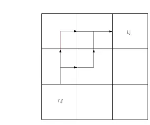
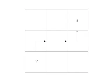
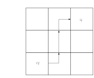
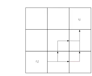
Although the FMM algorithm has been completed in three dimensions, figures 4.1 through

4.4, below, show a two dimensional depiction, for visual clarity, of the particle transport

(32)

i',j'

i,j

Figure 4.1: Two Dimensional Representation of Fn(i,j)(i0_,j0₎_,y,x for an Ordinate in the Primary

(33)

i',j'

i,j

Figure 4.2: Two Dimensional Representation of Fn(i,j)(i0_,j0₎_,y,y for an Ordinate in the Primary

(34)

i',j'

i,j

Figure 4.3: Two Dimensional Representation ofFn(i,j)(i0_,j0₎_,x,x for an Ordinate in the Primary

(35)

i',j'

i,j

Figure 4.4: Two Dimensional Representation of Fn(i,j)(i0_,j0₎_,x,y for an Ordinate in the Primary

Octant

It can be seen from a three dimensional extension of figures 4.1 through 4.4 how the element

Fn(i,j,k)(i0_,j0_,k0₎_,di,df can then be used to construct each of the four ITMM matrix operators in a

computationally efficient manner by avoiding repeat calculations since it represents the relation of the outgoing angular flux at any face in a domain to the incoming flux at any other face.

For an angular flux emergent from the face of one cell and incident on the face of another

cell in a three dimensional system, there are nine distinct elements of F resulting from three possible emergent faces and three possible incident faces. To accumulate values into each ITMM

operator, the only remaining calculation (after the calculation of the appropriate element ofF)

is to multiply Fn(i,j,k)(i0_,j0_,k0₎_,di,df by the respective values it is required to represent for the

emergent and incident cells. Recalling that the emergent cell is i0, j0, k0 and the incident cell

is i, j, k, the respective operators require multiplication ofFn(i,j,k)(i0_,j0_,k0₎_,di,df by the single cell

(36)

Table 4.1: Emergent and Incident Multipliers ofFn(i,j,k)(i0_,j0_,k0₎_,di,df for Construction of ITMM

Operators

Operator Emergent Cell Multiplier Incident Cell Multiplier

Jφ jψ,di,i0_,j0_,k0c_i0_,j0_,k0 k_φ,df,i,j,k

Jψ jψ,di,i0_,j0_,k0c_i0_,j0_,k0 k_ψ,d₁_→_df,i,j,k

Kφ kψ,d1→di,i0_,j0_,k0 k_φ,df,i,j,k

Kψ kψ,d1→di,i0_,j0_,k0 k_ψ,d₁_→_df,i,j,k

From equations 3.6 and 3.7, it can be seen how each single cell operator shown in Table 4.1

has a different value based on the direction it is required to represent, hence the necessity of nine distinct elements ofF representing particle transport from the faces of the emergent cell

to the to the faces of the incident cell in a three dimensional system.

The calculation of each element of F may appear to be computationally expensive due to

the sheer number of paths that a particle can travel from an emergent face to an incident

face, especially as the number of intervening cells grows. The FMM algorithm, however, avoids repeat calculations in the elements ofF (just as it avoids repeat calculations for matrix operator

elements by using F) by recognizing that each path is simply an extension of a previously

traversed path whoseF elements have already been computed. A path to a face of an adjacent cell from a face of a cell for which the element of F has already been calculated only needs

the respective elements of F to be multiplied by the appropriate value of kψ for each adjacent

cell. In this manner, single cell operators, or, more specifically, single cell values of kψ, are

compounded along a path to create an element ofF.

Each ITMM operator can then be constructed from elements ofF as follows.

The matrix operator Jφ, of dimensions (I x J x K) x (I x J x K)

Jφ=



  

jφ,1,1,1c1,1,1 · · · jψ,I,J,KcI,J,KFn(1,1,1)(I,J,K)kφ,1,1,1

..

. . .. ...

jψ,1,1,1c1,1,1Fn(I,J,K)(1,1,1)kφ,I,J,K · · · jφ,I,J,KcI,J,K



  

(37)

where

j_ψ,₍_i0_,j0_,k0₎c_i0_,j0_,k0F_n₍_i,j,k₎₍_i0_,j0_,k0₎k_φ,₍_i,j,k₎=j_ψ,x,₍_i0_,j0_,k0₎c_i0_,j0_,k0F_n₍_i,j,k₎₍_i0_,j0_,k0₎_,x,xk_φ,x,₍_i,j,k₎+ j_ψ,x,₍_i0_,j0_,k0₎c_i0_,j0_,k0F_n₍_i,j,k₎₍_i0_,j0_,k0₎_,x,yk_φ,y,₍_i,j,k₎+j_ψ,x,₍_i0_,j0_,k0₎c_i0_,j0_,k0F_n₍_i,j,k₎₍_i0_,j0_,k0₎_,x,zk_φ,z,₍_i,j,k₎+ j_ψ,y,₍_i0_,j0_,k0₎c_i0_,j0_,k0F_n₍_i,j,k₎₍_i0_,j0_,k0₎_,y,xk_φ,x,₍_i,j,k₎+j_ψ,y,₍_i0_,j0_,k0₎c_i0_,j0_,k0F_n₍_i,j,k₎₍_i0_,j0_,k0₎_,y,yk_φ,y,₍_i,j,k₎+

jψ,y,(i0_,j0_,k0₎c_i0_,j0_,k0F_n₍_i,j,k₎₍_i0_,j0_,k0₎_,y,zk_φ,z,₍_i,j,k₎+j_ψ,z,₍_i0_,j0_,k0₎c_i0_,j0_,k0F_n₍_i,j,k₎₍_i0_,j0_,k0₎_,z,xk_φ,x,₍_i,j,k₎+ jψ,z,(i0_,j0_,k0₎c_i0_,j0_,k0F_n₍_i,j,k₎₍_i0_,j0_,k0₎_,z,yk_φ,y,₍_i,j,k₎+j_ψ,z,₍_i0_,j0_,k0₎c_i0_,j0_,k0F_n₍_i,j,k₎₍_i0_,j0_,k0₎_,z,zk_φ,z,₍_i,j,k₎.

(4.5)

It is important to note that diagonal elements of Jφ do not use an element of F in their construction. This is because the diagonal elements represent the effect of the cell averaged

distributed source in a cell on the cell averaged scalar flux in the same cell. Since there is no

transport to account for between cells, no element of F is used and the single cell operator jφ

is used instead of jψ on the diagonal elements.

The matrix operator Jψ, of dimensions (D) x 2(IJ + JK + IK) x (I x J x K)

Jψ =

              

jψ,n,1,1,1c1,1,1Fn(1,1,1)(1,1,1)kψ,n,1,1,1 · · · jψ,n,I,J,KcI,J,KFn(1,1,1)(I,J,K)kψ,n,1,1,1

..

. · · · ...

jψ,n,1,1,1c1,1,1Fn(I,J,K)(1,1,1)kψ,n,I,J,K · · · jψ,n,I,J,KcI,J,KFn(I,J,K)(I,J,K)kψ,n,I,J,K

..

. · · · ...

jψ,N,1,1,1c1,1,1FN(1,1,1)(1,1,1)kψ,N,1,1,1 · · · jψ,N,I,J,KcI,J,KFN(1,1,1)(I,J,K)kψ,N,1,1,1

..

. · · · ...

jψ,N,1,1,1c1,1,1FN(I,J,K)(1,1,1)kψ,N,I,J,K · · · jψ,N,I,J,KcI,J,KFN(I,J,K)(I,J,K)kψ,N,I,J,K

               (4.6)

where, if considering the exiting x-face of the final cell and analogously for the exiting y-face

and z-face of the final cell,

jψ,(i0_,j0_,k0₎c_i0_,j0_,k0F_n₍_i,j,k₎₍_i0_,j0_,k0₎k_ψ,₍_i,j,k₎ =j_ψ,x,₍_i0_,j0_,k0₎c_i0_,j0_,k0F_n₍_i,j,k₎₍_i0_,j0_,k0₎_,x,xk_ψ,x_→_x,₍_i,j,k₎+ jψ,x,(i0_,j0_,k0₎c_i0_,j0_,k0F_n₍_i,j,k₎₍_i0_,j0_,k0₎_,x,yk_ψ,y_→_x,₍_i,j,k₎+j_ψ,x,₍_i0_,j0_,k0₎c_i0_,j0_,k0F_n₍_i,j,k₎₍_i0_,j0_,k0₎_,x,zk_ψ,z_→_x,₍_i,j,k₎+ jψ,y,(i0_,j0_,k0₎c_i0_,j0_,k0F_n₍_i,j,k₎₍_i0_,j0_,k0₎_,y,xk_ψ,x_→_x,₍_i,j,k₎+j_ψ,y,₍_i0_,j0_,k0₎c_i0_,j0_,k0F_n₍_i,j,k₎₍_i0_,j0_,k0₎_,y,yk_ψ,y_→_x,₍_i,j,k₎+ j_ψ,y,₍_i0_,j0_,k0₎c_i0_,j0_,k0F_n₍_i,j,k₎₍_i0_,j0_,k0₎_,y,zk_ψ,z_→_x,₍_i,j,k₎+j_ψ,z,₍_i0_,j0_,k0₎c_i0_,j0_,k0F_n₍_i,j,k₎₍_i0_,j0_,k0₎_,z,xk_ψ,x_→_x,₍_i,j,k₎+ j_ψ,z,₍_i0_,j0_,k0₎c_i0_,j0_,k0F_n₍_i,j,k₎₍_i0_,j0_,k0₎_,z,yk_ψ,y_→_x,₍_i,j,k₎+j_ψ,z,₍_i0_,j0_,k0₎c_i0_,j0_,k0F_n₍_i,j,k₎₍_i0_,j0_,k0₎_,z,zk_ψ,z_→_x,₍_i,j,k₎.

(4.7)

(38)

(D) Kφ =               

kψ,n,1,1,1Fn(1,1,1)(1,1,1)kφ,n,1,1,1 · · · kψ,n,1,1,1Fn(1,1,1)(I,J,K)kφ,n,1,1,1

..

. · · · ...

kψ,n,1,1,1Fn(I,J,K)(1,1,1)kφ,n,I,J,K · · · kψ,n,I,J,KFn(I,J,K)(I,J,K)kφ,n,I,J,K

..

. · · · ...

kψ,N,1,1,1FN(1,1,1)(1,1,1)kφ,N,1,1,1 · · · kψ,N,I,J,KFN(1,1,1)(I,J,K)kφ,N,1,1,1

..

. · · · ...

kψ,N,1,1,1FN(I,J,K)(1,1,1)kφ,N,I,J,K · · · kψ,N,I,J,KFN(I,J,K)(I,J,K)kφ,N,I,J,K

               T (4.8)

where, if considering the entering x-face of the initial cell and analogously for the entering y-face and z-face of the initial cell,

k_ψ,₍_i0_,j0_,k0₎F_n₍_i,j,k₎₍_i0_,j0_,k0₎k_φ,₍_i,j,k₎=k_ψ,x_→_x,₍_i0_,j0_,k0₎F_n₍_i,j,k₎₍_i0_,j0_,k0₎_,x,xk_φ,x,₍_i,j,k₎+

k_ψ,x→x,(i0_,j0_,k0₎F_n₍_i,j,k₎₍_i0_,j0_,k0₎_,x,yk_φ,y,₍_i,j,k₎+k_ψ,x_→_x,₍_i0_,j0_,k0₎F_n₍_i,j,k₎₍_i0_,j0_,k0₎_,x,zk_φ,z,₍_i,j,k₎+

kψ,x→y,(i0_,j0_,k0₎F_n₍_i,j,k₎₍_i0_,j0_,k0₎_,y,xk_φ,x,₍_i,j,k₎+k_ψ,x_→_y,₍_i0_,j0_,k0₎F_n₍_i,j,k₎₍_i0_,j0_,k0₎_,y,yk_φ,y,₍_i,j,k₎+ kψ,x→y,(i0_,j0_,k0₎F_n₍_i,j,k₎₍_i0_,j0_,k0₎_,y,zk_φ,z,₍_i,j,k₎+k_ψ,x_→_z,₍_i0_,j0_,k0₎F_n₍_i,j,k₎₍_i0_,j0_,k0₎_,z,xk_φ,x,₍_i,j,k₎+