Adaptive Clock Design for Memory Intensive 3D Integrated Circuits.

(1)

ABSTRACT

CHEN, XI. Adaptive Clock Design for Memory Intensive 3D Integrated Circuits. (Under the direction of Dr. W. Rhett Davis.)

Three-dimensional integrated circuit (3D IC) technology provides promising benefits for

advanced digital system designs. The technology not only helps to overcome the interconnect

wire delay barrier by greatly shortening the wire length from a 2D system, but also provides

a solution to the well-known memory wall problem by stacking multiple logic and memory

dies and connecting them with Through-Silicon-Vias (TSVs). All these features make 3D IC

technology an attractive option for the memory intensive integrated system.

Clock distribution is critical to a digital system design. When a system is implemented in

3D technologies, it is more challenging to control the clock skew due to cross-die process

variations, high thermal gradients and non-idealities of TSVs. Previous de-skew techniques

for 2D ICs, like delay-buffer insertion and active de-skew, introduce large overhead, require

complicated analysis, and are unable to compensate the clock distribution errors caused by

TSVs and cross-die variations in 3D ICs. Recently proposed 3D clock network designs either

do not have the capability to handle cross-tier variations, or oversimplify the effects of TSVs.

To implement accurate and balanced clock distribution in 3D ICs, a new adaptive clock

topology and de-skew technique are needed.

In this work, new technologies are developed to handle the challenges in 3D clock

distribution. Firstly, a new 3D clock distribution topology without H-tree structure is

proposed to achieve high quality and good cost-efficiency. Secondly, a novel return-signal

(2)

based tunable-delay-buffer (TDB) circuit is designed that is tunable in 360 degrees and has

good tolerance to process, voltage, and temperature (PVT) variations. Based on these

techniques, an accurate and highly adaptive clock distribution network can be implemented

in 3D integrated systems.

The proposed adaptive clock design technologies were validated in a chip fabricated in the

IBM 7RF 180nm CMOS process. Three transmission line based clock paths with different

wire lengths (1.5mm, 3mm, and 4.5mm) were created for testing the return-signal de-skew

technology. The measurement results show that, at 1GHz clock frequency, the de-skew

technology is able to reduce the clock skews from 440ps to 40ps.

In order to evaluate the effectiveness of the proposed adaptive clock design techniques,

design case study is performed. Moreover, a design optimization flow based on thermal

profiles is developed to minimize the power and area overhead of the TDB insertion and

further improves the adaptive clock network.

In addition to the adaptive clock design methodology, this work also includes the

development of other tools and techniques to facilitate memory-intensive 3D IC designs.

Memory models, a process-design-kit (PDK) and design tools are developed. A memory

generator tool is developed based on timing, power models and 3D PDK. An SRAM chip

with on-chip access time measurement was also fabricated in a real process and it proves the

(3)

(4)

Adaptive Clock Design for Memory Intensive 3D Integrated Circuits

by Xi Chen

A dissertation submitted to the Graduate Faculty of North Carolina State University

in partial fulfillment of the requirements for the degree of

Doctor of Philosophy

Electrical Engineering

Raleigh, North Carolina

2012

APPROVED BY:

_______________________ _______________________ Dr. W. Rhett Davis Dr. Paul D. Franzon

Committee Chair

(5)

(6)

BIOGRAPHY

Xi Chen received the B.S. and M.S. degrees in Electrical Engineering from Zhejiang

University, Hangzhou, China, in 2003 and 2006, respectively. He is currently working

toward the Ph.D. degree in the Department of Electrical and Computer Engineering, North

(7)

ACKNOWLEDGMENTS

First of all, I would like to thank my advisor, Dr. W. Rhett Davis, for offering me the greatest

support and guidance during my whole Ph.D. study. His insights and enthusiasm in research

are always inspiring me. It is my great fortune to have the opportunity working in this

friendly and open mined research group directed by Dr. Davis.

I also would like to thank Dr. Paul Franzon for giving me advice and guidance on

developing research ideas, and providing many support. I would like to express my

appreciation to Dr. Griff Bilbro and Dr. Douglas Reeves for being my committee and

offering valuable advice. Thanks for Dr. Lei Luo for very helpful discussion and technical

guidance on my work.

I would like to thank Dr. Steve Lipa for the help with chip bonding, test board design, and

software environment management in several projects. I also would like to thank for the

people from the MUSE group and other Electronic Circuits and Systems research groups for

help and friendship.

Finally, I want to extend my deepest gratitude to my parents for their unconditional

support. I greatly appreciate my wife for her endless love and extreme support through these

(8)

LIST OF TABLES

Table 3.1 PLL performance deviations... 40

Table 4.1 Chip summary and measured data ... 59

Table 5.1 Power consumption of different topologies... 70

Table 5.2 Routing area consumption of different topologies ... 70

Table 6.1 Current consumption of DDR memory with various configurations ... 87

(11)

LIST OF FIGURES

Figure 1.1 Interconnect delay vs. feature size [1.1]... 2

Figure 1.2 3D memory intensive system implementation ... 4

Figure 1.3 (a) Cross-tier variations, (b) thermal variations [1.10], and (c) parasitics of TSV [1.11] ... 7

Figure 2.1 Profile of MIT Lincoln Lab 3D SOI Process [2.1]... 13

Figure 2.2 SEM photograph of MITLL 3D IC process with 3 tiers [2.2]... 13

Figure 2.3 3D integration SRAM stacking on the 80 Core TFLOP chip [2.3]... 15

Figure 2.4 3D-stacked DRAM on CPU with ranks split across multiple layers [2.4].... 16

Figure 2.5 Conventional clock distribution topology [2.7]... 17

Figure 2.6 (a) Clock Domains and (b) Clock generator hierarchy for a 8-Core Intel Xeon® Processor [2.18]... 18

Figure 2.7 Clock generation for a Intel Nehalem® processor [2.19]... 19

Figure 2.8 Traditional TDB implementation [2.10] and cascading structure ... 20

Figure 2.9 Traditional active de-skew topology with reference distribution... 21

Figure 2.10 (a) Clock distribution hierarchy and (b) de-skew architecture for an Itanium® 2 Processor [2.11]... 22

Figure 2.11 (a) Phase compare structure and (b) region-based active de-skew topology [2.12]... 23

Figure 2.12 (a) Separated 2D clock [2.13], (b) 3D synthesized clock [2.14], and (c) shared global clock [2.16]... 24

Figure 3.1 Traditional H-tree clock distribution ... 27

Figure 3.2 (a) Proposed 3D clock distribution topology and (b) implementation example ... 28

Figure 3.3 Simplified diagram of the proposed return-signal de-skew technique... 32

Figure 3.4 Timing diagram of the return-signal active de-skew... 33

Figure 3.5 De-skew transient simulation results... 34

Figure 3.6 Simplified topologies of direct phase mixer... 35

Figure 3.7 Simulated linearity performance under PVT variations ... 36

Figure 3.8 TDB delay with different input rising time (Tr) and clock period (Tp)... 37

Figure 3.9 TDB linearity with different input rising times and loading capacitances .... 38

Figure 3.10 PLL frequency synthesizer and LC, Ring VCO topologies ... 39

Figure 3.11 Adaptive PLL implementation ... 41

Figure 4.1 Schematic of the 1.5mm clock distribution block ... 44

Figure 4.2 Schematic of (a) the Tunable-delay-buffer and (b) the comparator ... 46

Figure 4.3 Transient simulation waveforms of the phase-mixer TDB ... 47

Figure 4.4 Circuit topology of phase comparator and control counters ... 48

Figure 4.5 Transfer function of the control counter... 49

(12)

Figure 4.7 Schematic of the adaptive PLL frequency synthesizer... 51

Figure 4.8 Cross section and top view of the transmission line clock wire layout... 52

Figure 4.9 Die photo of the test chip... 53

Figure 4.10 Test print circuit board with chip directly bonded ... 54

Figure 4.11 Test equipment setup diagram for timing measurement ... 55

Figure 4.12 Lab equipments setup ... 56

Figure 4.13 Measured waveforms of three paths without de-skew ... 57

Figure 4.14 Measured waveforms of three paths with return-signal de-skew activated 58 Figure 5.1 Thermal Optimized Clock Network Design flow framework ... 61

Figure 5.2 Design optimization flow ... 62

Figure 5.3 Global clock tree before partition... 64

Figure 5.4 Thermal profiles for two stacking tiers ... 65

Figure 5.5 Delay distributions of two stacking tiers before partition ... 66

Figure 5.6 Clock distributions after regular partition ... 66

Figure 5.7 Skews of two tiers after regular partition ... 67

Figure 5.8 Simulated skew under different clock region sizes and TDB tuning steps ... 68

Figure 5.9 Clock distributions after thermal optimized partition ... 69

Figure 5.10 Skews of two tiers after thermal optimized partition ... 69

Figure 5.11 (a) Power, (b) routing area of clock and (c) skew performance compare ... 71

Figure 6.1 2D, memory-on-logic and multi-tier 3D memory implementation topologies ... 74

Figure 6.2 CAD tools required for 3D memory design ... 75

Figure 6.3 Hierarchical SRAM architecture ... 78

Figure 6.4 Word-line split and Bit-line split structures of 3D memory sub-array... 79

Figure 6.5 Word line partitioning (a) and Bit line partitioning (b) modeling... 81

Figure 6.6 3D SRAM Timing Analysis based on 45nm 3D FreePDK... 84

Figure 6.7 Current consumption of DDR products under different working status ... 88

Figure 6.8 Illustration of layer and 3D vias definitions in 3D FreePDK ... 89

Figure 6.9 3D via connection example of 3D 45nm FreePDK... 90

Figure 6.10 Flow chart of the 3D PDK compilation... 91

Figure 6.11 Working principle of 3D memory generator ... 92

Figure 6.12 Skeleton memory layout generation:... 93

Figure 7.1 Topology of 3D SRAM and access time measurement test chip ... 97

(13)

Chapter 1

Introduction

1.1 Motivation

The relationship known as Moore’s Law predicts that the number of transistors on a chip

doubles about every two years, and the chip complexity doubles every 18 months. This law

drives transistor devices to shrink significantly. Though device size becomes smaller, chip

size is continually increasing due to the growing demand for functionality and higher

performance.

Recent experiments show that, as technology scales, interconnects become more

significant limiting factor to performance and power dissipation of a chip. Wires get closer to

each other, and the length of interconnect increases as a result of larger die size and

decreasing feature size. Because wire thickness does not shrink in the same scale as device

size reduces, interconnect capacitance and resistance increase while device parasitics reduce.

As shown in Figure 1.1, delay due to the global interconnects increases exponentially as the

feature size decreases [1.1]. The increase is more significant without repeaters. Longer

interconnects require more repeaters to be inserted to achieve timing closure and signal

(14)

consumption. P. Saxena et al [1.2] expects that if the current trends continue, 35% of the total

cells will be repeaters in 45nm technology node and this number will increase to 70% in

32nm technology node. The difficulty is that interconnect behavior and the number of

repeaters are hard to predict before detailed physical design. There is an urgent need for

innovative design technologies that can reduce interconnect wire lengths. One potential

solution is to stack integrated circuits vertically, thereby reducing wire lengths. This

technique is commonly called 3D IC technology. This work explores new techniques to

enable 3D ICs.

Figure 1.1 Interconnect delay vs. feature size [1.1]

Specifically, this work develops a new clock methodology to help solve the so-called

“memory wall”. The memory wall arises because of the increasing difference in speeds

(15)

processor can be starved of data even at the processor–cache interface, especially if the

processor is being designed to operate at a much higher speed than the cache. If the processor

is designed to operate at 16 GHz and higher, the so-called memory wall can be observed at

the processor–cache interface as well. New solutions to the problem need to be extensively

developed.

This work proposes that a potential solution to the memory-wall problem is to stack

high-speed memory on top of high-high-speed logic using 3D IC techniques. A high-high-speed clock

distribution approach is needed to realize such a system. Here we introduce 3D IC

technologies and the challenges to clock-design in 3D ICs.

1.2 Three-dimensional IC Technologies

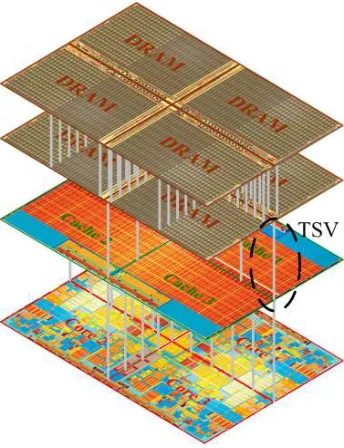
Three-dimensional integrated circuit (3D IC) technology has demonstrated great potential of

improving the performance of advanced memory intensive system design. It overcomes the

interconnect wire delay barrier by greatly shortening the wire length from 2D system [1.4].

3D IC technology can solve the well-known memory wall problem [1.5] by staking multiple

dies and connecting them with Through-Silicon-Vias (TSVs) [1.6] (Figure 1.2). In this way,

massive interconnect bandwidth between logic and memory is provided. 3D ICs also

significantly reduce memory access latency and I/O driver power consumption compared to

general multi-chip system [1.7]. All these features make 3D IC technology attractive for

(16)

Figure 1.2 3D memory intensive system implementation

1.2.1 3D IC overview

There are a number of different approaches when 3D IC integration technology is considered.

Depending on the assembly method, they can refer to die-level integration, wafer-level

integration, or device-level integration [1.8].

In die-level integration, wafers are processed, cut into dies first, and then aligned and

stacked to either another die or a wafer. The dies are electrically connected using

wirebonding or microbumps. Die-level integration has a known good yield as each die has its

own inputs and outputs so that they can be fully tested before stacking. Die-level integration

has been most mature 3D integration technology that has been widely used in 3D packaging

(17)

In wafer-level integration, wafers are stacked first and then cut into dies. The inputs and

outputs of the chip are usually on top tier to communicate with the outside of the chip.

Through-silicon vias (TSVs) are used to communicate among different tiers. Tier is defined

as each active layer and its associated metals layers in this work. Wafers can have SOI

substrate or thicker bulk substrate. Using TSVs, wafer scale integration provides high via

density, which can achieve higher performance while it results in a higher cost. Wafer-level

3D IC process technologies can be categorized as via-last or via-first process depending on

the processing order of the 3D vias. This dissertation focuses on the wafer-level integration.

In device-level integration, also called monolithic 3D integration, active layers are bonded

vertically to form stacked npn junctions and results in vertical transistors after etching.

Monolithic 3D IC can achieve highest via density. However, it requires more complex

fabrication process and is unlikely to be used for mass-production.

1.2.2 Challenges of clock design in 3D IC

The clock signal timing reference is critical to both system reliability and performance. In

aggressively scaled technologies, the control of clock skew becomes increasingly important.

Advanced memory intensive system requires specific clock design for high accessing speed.

When the system is implemented in 3D, the clock design becomes more complex and

challenging.

3D IC technologies bring us some benefits to improve the performance of digital system.

However, they also create new challenges for circuit design, especially for high quality clock

(18)

First, 3D integration is going to have larger process variations. In a 3D integration,

especially a heterogeneous integration, cross-die process variations will increase the clock

skews if the sequential elements in the same clock domain are located on different tiers.

Figure 1.3(a) shows the MOS transistor I-V performance of MITLL 3D process [1.10]. The

results indicate that large differences exist cross the tiers.

Secondly, significant thermal gradients exist in 3D integrations. A 3D integration will lead

to a higher heat density and moves some active devices further away from the heat-sink. The

increased thermal gradients will result in significant clock skews. Another set of testing

results from MITLL in Figure 1.3(b) shows that, in three tiers stacking, the temperature

increases quickly with the tier stacking goes up [1.10].

In addition, the TSVs introduce more parasitic parameters and uncertainties. Due to

parasitics, TSVs can degrade clock signal quality and increase skews. Also TSVs can absorb

noise from substrate. In addition, TSVs make it difficult to design a highly symmetric clock

distribution As we can find in the basic TSV model shown in Figure 1.3(c), the parasitic

parameters will cause extra RC delay, signal distortion, and absorbing noise from the

(19)

Ids

[A

]

Vds [V]

I/V Curve of NMOS (Vgs=1.5V, W/L=6um/0.2um)

(a)

Power [W]

T

e

rm

p

e

ra

tu

re

[

℃

]

Thermal Performance

(b)

Cgc Cvc

Lsc Rv

Lv

(c)

(20)

1.3 Research Contributions

This work proposes novel technologies and systematic design flow to handle the

complexities and challenges in the clock designs for 3D memory intensive systems. The key

contributions include,

Developed new cost-effective and robust adaptive clock distribution technologies (Chapter 3).

Firstly, an efficient clock distribution topology without need of balanced H-tree is

proposed. Secondly, a novel tunable-delay-buffer (TDB) circuit which is tunable in 360

degree and robust under PVT variations is developed. Thirdly, a new active de-skew method

are developed in order to handle the cross-die variations, thermal gradients, and wiring

asymmetry.

Designed and fabricated a test chip for demonstrating the proposed adaptive clock distribution technologies (Chapter 4).

A test chip was developed to validate the proposed return-signal de-skew technique. The

test chip was designed and fabricated on IBM 7RF 180nm CMOS process. The testing results

show that the proposed technologies are effective in reducing the clock skew.

(21)

A design optimization flow is developed in order to figure out the optimal clock regions

whose dimensions are inversely proportional to the thermal gradients within them. The clock

regions will be adaptively partitioned, and the TDB insertions and the return signals paths in

the physical design are updated accordingly. At the end of the flow, the optimal clock regions

based on the thermal profiles are derived.

Proposed new design methodologies for 3D memories (Chapter 6).

Physically-based modeling and delay analysis approaches are proposed to explore the 3D

SRAM designs. The new approaches can be used to optimize the 3D SRAM timing

performance at both sub-array and system level. An open-source 3D Process Design Kit

(3DPDK) and a 3D memory generator to facilitate 3DIC designs in standard IC design tools.

Designed and taped out a 3D SRAM chip with a novel on-chip access-time measurement circuit (Chapter 7).

An SRAM chip was designed and fabricated in a 0.18µm 3D silicon-on-insulator (SOI)

technology. A novel delay-locked loop (DLL) based access time measurement circuit was

designed on-chip for accurate evaluation of the 3D SRAM performance. The results show

(22)

1.4 Dissertation Overview

This dissertation is organized as follows: Chapter 2 presents an overview of the existing 3D

integrated circuit technologies and previous clock design techniques. Chapter 3 proposes the

new clock distribution topology and the novel de-skew technique for adaptive 3D clock

network design. Chapter 4 demonstrates the 180nm adaptive clock test chip design and

measurements. Chapter 5 discusses the design case for optimization and TDB insertion.

Chapter 6 introduces the 3D memory modeling and design tools. A 3D SRAM test chip with

access time measurement is presented in Chapter 7. Chapter 8 summarizes the main

contributions of this work and discusses the future work.

References

[1.1] ITRS Roadmap, available at http://www.itrs.net.

[1.2] P. Saxena, et al., “Repeater scaling and its impact on CAD”, IEEE Tran. on Comp. Aided Design of Integrated Circuits and Systems, pp.451 – 463, April 2004.

[1.3] W. A. Wulf and S. A. McKee, “Hitting the memory wall: Implications of the obvious,” ACM SIGARCH Comput. Architect. News, vol. 23, no. 1, pp. 20–24, Mar. 1995.

[1.4] K. Banerjee, S. J. Souri, P. Kapur, K. C. Saraswat, “3-D ICs: a novel chip design for improving deep-submicrometer interconnect performance and systems-on-chip integration”, Proceedings of the IEEE, pp. 602 – 633, May 2001.

[1.5] W.A. Wulf and S.A. McKee, “Hitting the memory wall: Implications of the obvious,” ACM SIGARCH Computer Architecture News, vol. 23, no. 1, pp. 20–24, March 1995.

[1.6] S. Borkar, “3D integration for energy efficient system design”, Symposium on VLSI Technology, 2009, 16-18 pp.58 – 59, June 2009.

(23)

[1.8] W. R. Davis, et al., “Demystifying 3D ICs: the Pros and Cons of Going Vertical,” IEEE Design & Test of Computers, Vol. 22, Issue 6, pp. 498-510, 2005.

[1.9] S. K. Lim, “Physical design for 3D system on package,” IEEE Design & Test of Computers, vol. 22, pp. 532-539, 2005.

[1.10] T.W. Chen, et al., “Thermal modeling and device noise properties of three-dimensional–soi technology”, IEEE Tran. on Electron Devices, Vol. 56, No. 4, pp.656-664, April 2009

(24)

Chapter 2

Literature Review and Related Work

2.1 3D Integration Technology

This section reviews the 3D IC manufacturing technologies that have influenced this work.

2.1.1 MIT Lincoln Lab 3D process

One of the major 3D IC processes that have been explored in our work is MITLL 3D

integration process. MITLL has been the first widely available wafer-level 3D IC process and

provides tightly integrated 3D IC process with high yield inter-tier 3D vias.

MITLL 3D IC technology is a 0.18um process based on fully depleted silicon on insulator

(FD SOI) fabrication. It is three tier 3D process with a face-to-face bonding for the base tier,

Tier 1 and Tier 2, and a face-to-bottom bonding for Tier 1 and Tier 3. Each tier is about

10um thick and has one poly layer and three metal layers. The tiers are directly connected by

tungsten 3D vias. The resulting 3D via including blockage is about 2um by 2um in dimension,

and their capacitance is comparable with metal capacitance. For instance, the parasitic

(25)

similar to the coupling capacitance between two 3D inter-tier vias. An illustration of the

cross section is shown in Figure 2.1 [2.1], and the SEM photograph of MITLL 3D IC process

is shown in Figure 2.2 [2.2].

TSV

Figure 2.1 Profile of MIT Lincoln Lab 3D SOI Process [2.1]

(26)

2.1.2 Tezzaron 3D process

The Tezzaron 3D IC process is 130 nm wafer-level 3D bulk CMOS process with 6 metal

layers including Cu layer for bonding per silicon tier. The 3D vias are formed before stacking

of silicon wafer. In this process, TSV is formed after transistors are created on each tier as in

conventional process, but before metal layers are deposited.

Tezzaron’s 3D IC process offers integration of multiple tiers with Tungsten Through

Silicon Via (TSV) connection with copper bonding. Tezzarons 3D IC is a wafer-level 3D

via-first bulk CMOS process with multiple tiers, six metal layers per tier including five

aluminum layers and one copper layer for copper bonding. Again, the TSV’s are formed after

transistors are created on each tier in Tezzaron’s process, and then metal layers are deposited

for wiring. Each upper tier is flipped, aligned, and bonded to lower tier. And then top tier is

thinned, grinded, and have copper deposition for the next tier stacking. After all the tiers are

stacked, the stack is inverted. As a result, all tiers are connected with the 3D vias composed

of tungsten TSVs and the copper bondpads, except the last two tier connections, which are

done with copper bondpads only.

2.1.3 Other processes and design cases

The 80 Core TFLOP system of Intel [2.3] demands more than 100GB/sec memory bandwidth.

Traditional SRAM was used to demonstrate the concept of 3D-stacked memory-on-processor

for this multi-core system. The SRAM has the same dimensions as the TFLOP chip. It is

(27)

the SRAM chip with a 3D interconnected memory bus as shown in Figure 2.3. Each SRAM

tile integrates 256KB of static memory and interface logic, and overall provides 20MB of

memory to the system. The stacked SRAM connects to an 82 core processor test chip, which

demonstrated > 1 TFLOP operation and a 90% reduction of memory access I/O power.

However, this design only supports two tiers stacking and is not flexible and economical

enough for more general 3D IC design.

Figure 2.3 3D integration SRAM stacking on the 80 Core TFLOP chip [2.3]

The more cost efficient 3D DRAM stacking for multi-core processors was proposed in

[2.4], based on a so-called “true” 3D DRAM concept. It uses the fine-grained 3D partitioning

strategy, and distributes each rank into all stacking tiers at the wordline/bitline level. The

design also separates the peripheral logic circuit and DRAM cells in different silicon layers

for best process performance based on the concept from [2.5]. The wordline/bitline

partitioning strategy is similar to the 3D SRAM partitioning structure talking in [2.6]. These

(28)

the fabrication of a relatively large amount of TSVs and the pitch of TSVs must be

comparable to the memory wordline/bitline pitch (e.g., hundreds or even tens of nm pitch).

This tends to put an increasingly stringent constraint on TSV pitch as the technology scales

down, particularly for DRAMs.

Figure 2.4 3D-stacked DRAM on CPU with ranks split across multiple layers [2.4]

2.2 Conventional Clock Designs

This section reviews the previous clocking methodologies that influenced this work.

2.2.1 General topology of clock system

Figure 2.5 shows the conventional clock distribution topology in digital system [2.7].

(29)

distribution is generally a balanced H-tree with active de-skew. At the end of global

distribution, there are many regional distribution networks, which are constructed as clock

grid or binary tree. The local distributions are generated by synthesis algorithm with clock

buffers insertion for timing optimization.

Figure 2.5 Conventional clock distribution topology [2.7]

For a complicated digital system, such as micro-processor, the task of distributing accurate

clock signals into a large chip area is very challenging. To achieve good reliability of the

clock signal for all circuit blocks, sometimes the clock distribution structure needs to be

divided into several domains (Figure 2.6 (a)). The clock signals will be resynchronized by a

specific phase-locked-loop (PLL) for each clock domain (Figure 2.6 (b)). For a large system

like multi-core processor, theses PLLs consume a significant amount of power, also

(30)

(a)

(b)

(31)

The clock networks for processors are generally implemented as cascading PLLs (Figure

2.7). A central PLL serves as a filter to attenuate the noise from reference clock signal. A

local PLL resynchronizes the clock signal distributed from the central PLL, and locks the

phase of feedback signal to the reference.

Figure 2.7 Clock generation for a Intel Nehalem® processor [2.19]

2.2.2 De-skew technologies

For de-skew purpose, some components with configurable delay are needed. A

tunable-delay-buffer (TDB) is generally used for this purpose. The traditional TDB controls

capacitance loading and current to achieve the delay tuning. These circuits are highly

sensitive to process and environmental variations. Traditional TDBs are usually cascaded in

the clock tree to achieve skew compensation (Figure 2.8). This structure requires the large

effort of delay distribution analysis.

Some techniques for reducing clock skew have been proposed. One is the sensor based

method. Non-uniform thermal distribution is a major source of clock skew [2.8]. By placing

(32)

delays correlated with the thermal profile by temperature sensors, it’s possible to partially

compensate the clock skew. The TDB used for skew compensation can be implemented as

analog tuning [2.9] or digital tuning [2.10]. The drawback of sensor based de-skew is that

when TDB insertion is made in more clock stages, design overhead increases largely, and the

error will accumulate across the whole clock path. Moreover, the TDB itself can be sensitive

to variations. This method heavily also relies on accurate modeling of thermal performance at

design stage and complicated analysis is required. Therefore, sensor based de-skew is not a

good choice for large scale and high performance design.

Root of clock tree

TD B

Regional clock distributions

Figure 2.8 Traditional TDB implementation [2.10] and cascading structure

Another method is to use active de-skew technique. In a high performance system like a

microprocessor, the skew requirement may be less than 10ps. In this case, the clock

distribution path is usually divided into several sections. At the global distribution level, the

active de-skew technique is usually used to provide a balanced clock signal to all circuit units

[2.7]. In this method, clock phases at loading points are continuously compared to the

(33)

shows, the regional clock is locked to a reference distributed from clock source or nearby

clock region. In this method, TDBs and phase comparators are needed for every clock region.

Phase Comparator

…

Clock Source

Global Distribution Regional Distribution

Reference from

clock source Reference from _{nearby region}

Figure 2.9 Traditional active de-skew topology with reference distribution

One way to distribute the accurate reference signal is to generate a separate reference clock

and distribute it in a highly balanced fashion [2.11]. Figure 2.10 shows the clock distribution

hierarchy and the de-skew architecture used in an Itanium® 2 Processor. In this topology, each clock region will be calibrated compared to the reference signal. The tuning code

settings for all TDBs (SLCB in the figure) will be stored in the fuse unit after the one-time

tuning happens at start-up process. The tuning setting can also be refreshed by the test unit

for any environmental condition change.

The other way is to create a hierarchical collection of phase comparators between the ends

of different global and regional routes [2.12] (Figure 2.11). With one zone locked as the

reference, each of the other zones is referred to the phase of a near-by zone. In this method,

the highly reliable global reference distribution can be avoided, but the error will accumulate

(34)

(a)

(b)

Figure 2.10 (a) Clock distribution hierarchy and (b) de-skew architecture for an Itanium® 2 Processor [2.11]

Unfortunately, both methods are sensitive to process and thermal variations, and neither of

them can compensate the asymmetry caused by TSVs. Therefore, previously proposed active

de-skew techniques are not suitable for 3D clock design. The clock signal for memory often

requires intentional skewing capability. When memory and logic are separated to different

stacking tiers for process optimization purpose, the clock design for memory intensive

(35)

(a) (b)

Figure 2.11 (a) Phase compare structure and (b) region-based active de-skew topology [2.12]

2.2.3 Previous 3D clock design cases

Extending the clock network design into three dimensions will cause new difficulties such as

worse process and thermal variation and asymmetry caused by non-ideal TSVs. In recent

years, several efforts have researched clock networks in 3DICs. In [2.13], clock trees are

designed for each tier with a standard 2D approach, and their delays are balanced by buffer

insertion at the root points (Figure 2.9a). Without the capability to handle cross-tier

variations, the skew of this case is up to 250ps in simulation.

In [2.14], the clock network routes the wires freely in three dimensional space through

updated algorithms (Figure 2.9b). However, as these routing algorithms oversimplify the

(36)

(a)

(b)

(c)

Figure 2.12 (a) Separated 2D clock [2.13], (b) 3D synthesized clock [2.14], and (c) shared global clock [2.16]

In [2.16] three simple test structures of 3D clock are fabricated in the MITLL 180nm SOI

(37)

performance in 3D. The authors of [2.9] also extend the design on analog sensors and TDBs

into 3DIC [2.17], but they do not provide solutions to deal with the non-ideality caused by

3D integration.

To handle 3D clock design challenges, appropriate distribution architecture, de-skew

techniques and optimization design methods are still open problems.

References

[2.1] MITLL Low-Power FDSOI CMOS Process Design Guide, Sep. 2008

[2.2] J. Burns et al. “A Wafer-Scale 3-D Circuit Integration Technology,” IEEE Transaction on Electronic Devices, Vol. 53, No. 10, pp. 2507-2516, Oct. 2006.

[2.3] S. Borkar, “3D integration for energy efficient system design”, Symposium on VLSI Technology, 2009, 16-18, pp. 58-59, Jun. 2009.

[2.4] G. Loh, “3D-stacked memory architecture for multi-core processors,” in Proceedings of the 35th ACM/IEEE Intl. Conf. on Computer Architecture, Jun. 2008.

[2.5] Tezzaron Semiconductors, 3D Stacked DRAM, http://www.tachyonsemi.com/memory/-Overview 3D DRAM.htm, 2008.

[2.6] Y.-F. Tsai, F. Wang, Y. Xie, N. Vijaykrishnan, and M. J. Irwin, “Design Space Exploration for 3-D Cache,” IEEE Transactions on Very Large Scale Integration (VLSI) Systems, vol. 16, pp. 444–455, Apr. 2008.

[2.7] S. Tam et al, “Clock generation and distribution for the first IA-64 microprocessor”, IEEE Journal of Solid-State Circuits, Volume: 35, Issue: 11, pp. 1545 – 1552, 2000,

[2.8] S.A. Bota et al, “Impact of Thermal Gradients on Clock Skew and Testing”, IEEE Design & Test of Computers, Volume: 23, Issue: 5, pp. 414 – 424, 2006.

[2.9] M. Mondal et al, “Mitigating Thermal Effects on Clock Skew with Dynamically Adaptive Drivers”, International Symposium on Quality Electronic Design, pp. 67 – 72, 2007.

(38)

[2.11] S. Tam, R. D. Limaye and U. N. Desai, “Clock Generation and Distribution for the 130-nm Itanium® 2 Processor with 6-MB On-Die L3 Cache”, IEEE Journal of Solid-State Circuits, Vol. 39, No. 4, Apr. 2004.

[2.12] P. Mahoney, et al., “Clock Distribution on a Dual-Core, Multi-Threaded Itanium®-Family Processor”, IEEE International Solid-State Circuits Conference, 2005.

[2.13] H. Hua, “Design and Verification Methodology for Complex Three-Dimensional Digital Integrated Circuit”, Ph.D. Dissertation, North Carolina State University, 2006.

[2.14] J. Minz, X. Zhao and S. K. Lim, “Buffered Clock Tree Synthesis for 3D ICs under Thermal Variations”, Asia and South Pacific Design Automation Conference, pp.504 – 509, 2008.

[2.15] D. Kung and R. Puri, “CAD challenges for 3D ICs”, Asia and South Pacific Design Automation Conference, pp. 421 – 422, Jan. 2009.

[2.16] V. F. Pavlidis, I. Savidis and E. G. Friedman, “Clock Distribution Networks for 3-D Integrated Circuits”, IEEE Custom Intergrated Circuits Conference, pp. 651 – 654, 2008.

[2.17] M. Mondal et al, “Thermally Robust Clocking Schemes for 3D Integrated Circuits”, Design, Automation & Test in Europe, pp. 1 – 6, 2007.

[2.18] S. Tam, J. Leung and R. Limaye, “Clock Generation & Distribution for a 45nm, 8 Core Xeon® Processor with 24MB Cache”, Symposium on VLSI Circuits, pp. 154 – 155, 2009.

(39)

Chapter 3

Adaptive 3D Clock Design

3.1 Efficient Clock Distribution Topology

3.1.1 Proposed 3D clock distribution

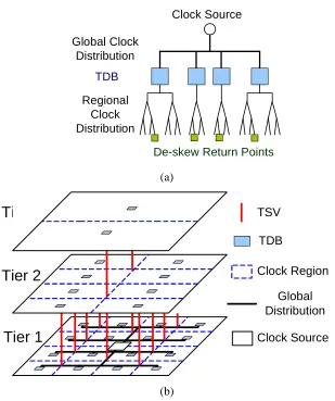
Traditionally, the global clock is distributed in an H-tree structure (Figure 3.1). The purpose

of this structure is to achieve highly balanced distribution delays among all routing path.

CLK_IN Clock

Buffer

Clock Loading

(40)

However, the required accurate matching of H-tree always suffers variations cross the die

area, especially in 3D integration environment. And the H-tree routing consumes large chip

area and power in cascading buffers.

Clock Source

TDB

De-skew Return Points

Global Clock Distribution

Regional Clock Distribution

(a)

Global Distribution Clock Region TSV

TDB

Tier 1

Tier 3

Clock Source

Tier 2

(b)

Figure 3.2 (a) Proposed 3D clock distribution topology and (b) implementation example

A new distribution topology without an H-tree is proposed to reduce routing complexity,

consume less power and minimize the impact of cross-tier variations in 3D ICs. As shown in

(41)

generator. Tunable-delay Buffers (TDBs) are placed in every circuit unit on all tiers and are

driven by the clock distribution network through TSVs. When the tuning range of TDBs

covers the full clock duty cycle, TDBs are only needed on the bottom layer of the clock tree

distribution. This will greatly reduce the design cost. Meanwhile, the proposed 3D clock

distribution topology will flexibly support all logic and memory domains with only one clock

generator. It avoids multiple Phase-Locked-Loops (PLLs) in traditional high performance

memory intensive systems [3.1] and greatly reduces area and power consumption.

3.1.2 Multi-phase clock

A multi-phase clock [3.2] is used to compensate the variations in the distribution network

and improve timing accuracy. In this topology, the clock source generates several parallel

clock signals with equal phase offsets which are all actively locked and referred to the

off-chip reference. With a multi-phase clock, variation tolerant TDBs can be realized by phase

interpolation [3.3]. Unlike a conventional SoC clock, which requires multiple PLL/DLLs to

synthesize regional clock signals with higher frequencies and tunable phases [3.1][3.4], the

proposed multi-phase clock can achieve frequency multiplication and precise phase tuning

without an extra PLL/DLL other than the clock generator. Therefore, in the proposed

topology, one clock source can drive the whole 3D system. The multi-phase clock generator

can be implemented as a DLL or ring oscillator PLL. For a 3D clock design, high-bandwidth

DLL operation is used to avoid the supply noise accumulation [3.5]. As device mismatch and

(42)

distributive DLL structure [3.7] and time-averaging technique [3.8] are also used to attenuate

the mismatch of multi-phase clock.

3.2 Return-Signal De-Skew

Traditional de-skew techniques can not handle the cross-die variations and 3D wiring

asymmetry. In this work, de-skew method based on return-signal is proposed to handle the

cross-die variations and unbalanced clock distribution which can not be calibrated by

previous technologies. The de-skew technology is supported by a new tunable-delay buffer

(TDB) design. Different from previous TDB applications, which rely on complicated

analysis and cause large design overhead, the new TDB can achieve 360 degree tuning range

and realize the skew compensation in a single stage. The TDB design for 3D clock is

variation tolerant and low cost. The circuit achieves accurate compensation by high tuning

resolution and good linearity.

To minimize the clock skew, TDBs located at all clock loading regions need to be

accurately in-phase. In this work, I propose a novel de-skew method. The simplified

functional diagram showing only one clock path is as Figure 3.3. The forward clock path

(blue line) distributes clock signal from source to loading point. In active de-skew process,

by tuning the delay of the TDB (TDB_L in Figure 3.3), we want to compensate the delays of

global and regional distribution and synchronize the phase at loading point (ΦLoading) to the

(43)

the forward path. By going through almost same routing path and same number of TSVs as

the forward signal, the return signal should have almost the same delay under all conditions.

At the Phase Comparator located close to the clock source, the return signal phase PL will be

compared with a reference signal phase Pref, which is delayed by a reference TDB (TDB_ref

in Figure 3.3) from the clock source. When phase difference exists between the two signals,

phase comparator incrementally sweep the control bits D of TDB_L until PL matches Pref,

and the control bits D_{of TDB_ref is the complementary code of D. That means the delay of}

TDB_L plus the delay of TDB_ref always equals to a full clock period. When PL matches Pref,

the phase ΦLoading at the loading point should be exactly in-phased to ΦSource at the clock

source. The proposed de-skew method has good adaptability to the cross-tier variations and

the asymmetry caused by TSVs. In addition, all the clock regions can be calibrated with only

one phase comparator, which saves large design overhead.

This return signal de-skew method has good adaptability to the asymmetry caused by

TSVs. Since all parasitic effects are included in the path, the de-skewing does not rely on

accurate TSV modeling and avoids the over-simplification in previous research. As all the

clock regions can be calibrated with one phase comparator, the return signal de-skew avoids

(44)

Figure 3.3 Simplified diagram of the proposed return-signal de-skew technique

An example timing diagram for the return-signal de-skew is shown as Figure 3.4. At

beginning status, in forward path, skew exists between loading and source. After the return

path delay, phase comparator detects phase error between returned signal phase PL and Pref,

which is delayed by TDB_ref from clock source. Because Phase Error is larger than zero, the

phase comparator incrementally sweeps the tuning code D of TDB_L, push the return signal

phase close to Pref. Since the control bit D

is complementary code of D, delay of TDB_ref

reduces accordingly. After several clock cycles, finally, returned phase PL and reference

phase Pref match and lock. Because TDB_ref plus TDB_L always equals to full clock period,

and forward path delay equals to return path delay, the total delay from source to loading will

be integral clock cycles. The phase at loading point is matched to clock source. The skew is

(45)

D D

D

D D

D

Figure 3.4 Timing diagram of the return-signal active de-skew

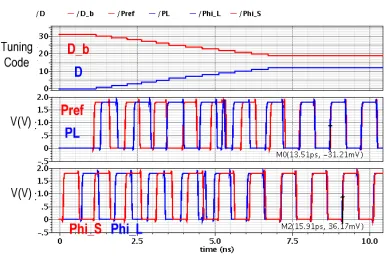
3.2.2 Behavioral simulation results

Figure 3.5 shows the simulation results of de-skew technology at 1GHz clock frequency. The

upper figure shows the change of the tuning codes D and D_{. The middle figure shows the}

waveforms of reference signal Pref and returned signal PL. The lower figure is the phases at

clock source (Phi_S) and at loading point (Phi_L). The results show the signals at source and

(46)

Figure 3.5 De-skew transient simulation results

3.3 Phase-Mixer TDB Design

3.3.1 Circuit structure

In this work, we use multi-phase clocking to enhance the capability of locking the phases of

the TDBs with the clock generator. A Phase Mixer based TDB (PM-TDB) circuit is designed

to compensate the skew in the clock distribution.

As shown in Figure 3.6, the PM-TDB consists of a phase multiplexer (MUX) and a phase

interpolator. By interpolating the multi-phase clock, delay of the PM-TDB can be tuned

(47)

degree and generating arbitrary delay within only one stage. This avoids the need for a highly

balanced H-tree and a large number of TDB insertions. This feature is very useful for the

asymmetrical 3D clock network design. Secondly, the circuit has good immunity to PVT

variations. Moreover, the TDB is convenient for regional clock gating and intentional skew

editing as it can be tuned individually without complex and inefficient delay analysis [3.9].

Phase mixer can achieve about 10ps tuning step. If smaller step is expected, fine tune stage

can be added into the TDB stage [3.4] [3.10][3.11].

└

In

te

rp

o

la

to

r

┴

M

ul

tip

le

xe

r

┘

Figure 3.6 Simplified topologies of direct phase mixer

A 5-bit controlled (including MUX and interpolator bits) quadrature phase mixer is

designed and simulated in a 45nm CMOS process. The loading structure for the circuit is

optimized for better slew-rate and linearity. As results show, the total power consumption for

one mixer is 125µW (eight times of minimum inverter) at 1GHz, and the silicon area is

(48)

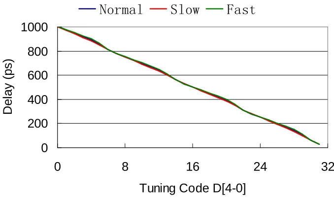
3.3.2 Variations tolerance validation

The most important specification for a phase mixer is the linearity. The simulated linearity

performance of the phase mixer based TDB under normal and worst PVT conditions at 1GHz

frequency are showing in Figure 3.7. We can see that although there are some deviations of

the delay transfer function, the linearity of phase mixer TDB is good enough for de-skew

purpose. The fundamental requirement for a TDB is that the delay transfer should be

monotonic. However, better linearity is good for minimizing static phase error when de-skew

is using.

0 200 400 600 800 1000

0 8 16 24 32

Tuning Code D[4-0]

D

e

la

y

(

p

s

)

Normal

Slow

Fast

Figure 3.7 Simulated linearity performance under PVT variations

For the analog interpolation used in phase mixer, generally the input rising time may

interfere the output delay value. As Figure 3.8 shows, in this work, the rising time (Tr) of the

(49)

range of frequencies to provide better design flexibility. Also showing in Figure 3.10, when

we reduce the clock period (Tp), the output delay reduce accordingly and as expected,

meanwhile, the delay transfer performance remains good linearity.

300 350 400 450 500 550 600 650

0 2 4 6 8

Tuning code

D

e

l

a

y

(

p

s

)

Tr=50ps Tr=150ps Tr=250ps Tp=750p Tp=500p

Figure 3.8 TDB delay with different input rising time (Tr) and clock period (Tp)

Figure 3.9 shows the TDB linearity performance in part of the continuous tuning range.

From this figure, we can find that, although the linearity of TDB is robust under different

input rising time, it suffers a large variation with the decreasing effective loading capacitance.

This result comes from another important design constrain for analog interpolation. To

(50)

at the output of TDB, we can achieve good linearity performance under a large PVT variation

range.

0 100 200 300 400 500 600

0 1 2 3 4 5 6 7 8

Tuning Code

D

e

l

a

y

(

p

s

)

Tr50p Tr150p Ideal CL80f CL160f CL=40f

Figure 3.9 TDB linearity with different input rising times and loading capacitances

3.4 Variation-tolerant Clock Generation

3.4.1 PLL frequency synthesizer

For the multi-phase clock generation, a PLL-based frequency synthesizer is usually used.

Analog PLL is still the major choice for high quality clock generation because its noise

(51)

under temperature and process variations. In this work, we would like to explore the variation

performance of PLL design, and the design method to improve the robustness of PLL.

Charge pump PLL frequency synthesizer can be implemented as two different styles as the

VCO design, which are LC VCO and Ring VCO. The topology of PLL and VCO are

showing in Figure 3.10. Multi-phase clock signals can be generated by dividing the

differential outputs of LC VCO, or directly from the outputs of the buffers in Ring VCO.

PFD

KPFD

F

ref Icp Icp Rz

C1 C2

KVCO /s

VCO

/N

F

out

F

fb F(s) Vtune b0 b1 b2 VDDVCO Ibias Cbp

LC VCO

+ - + + - + + - + + - +

Vtune Cbp

VDDVCO

(52)

3.4.2 Adaptive design for PVT variations

The PLL circuit performance is impacted by process and temperature variations. For instance,

from SPICE level simulation, the normalized bandwidth deviations of LC PLL and Ring PLL

are listed in the table below. It’s obvious that Ring PLL suffers much larger deviation

compared to LC PLL.

Table 3.1 PLL performance deviations

Bandwidth Positive Deviation Negative Deviation

LC-PLL 1.8% @FF Corner, High Temp -3.5% @SS Corner, Low Temp

Ring-PLL 21.5% @SS Corner, High Temp -13.5% @FF Corner, Low Temp

For adaptive PLL implementation, we can make charge pump current (Icp) and zero

resistor (Rz) in loop filter tunable to compensate variations of bandwidth and damping factor.

The general topology is shown in Figure 3.11. Traditionally, the tuning process relies on

complicated and unstable searching algorithms. The searching algorithms will take a long

time and has the risk to unlock.

In this work, we partition the variations space by process and temperature, and decide the

settings of Icp and Rz at design stage. This method avoids creating extra feedback loop and

searching in tuning. The partition information comes from process and temperature sensors

(53)

Figure 3.11 Adaptive PLL implementation

Based on the equations in Figure 3.11 and the simulation data in Table 3.1, we can find

that, with 30% tuning range of Icp, the bandwidth deviation of Ring-PLL can be constrained

within 10% of its nominal value.

References

[3.1] S. Tam, J. Leung and R. Limaye, “Clock Generation & Distribution for a 45nm, 8 Core Xeon® Processor with 24MB Cache”, Symposium on VLSI Circuits, pp. 154 – 155, 2009.

[3.2] K. Nose and M.Mizuno, “Parallel Clocking: A Multi-Phase Clock-Network for 10GHz SoC”, IEEE International Solid-State Circuits Conference, 2004.

[3.3] K. Yamguchi et al, “2.5GHz 4-phase Clock Generator with Scalable and No Feedback Loop Architecture”, IEEE International Solid-State Circuits Conference, 2001.

[3.4] T. Fischer et al, “A 90-nm Variable Frequency Clock System for a Power-Managed Itanium Architecture Processor”, IEEE Journal of Solid-State Circuits, Vol. 41, No. 1, pp. 218 – 228, Jan. 2006.

1 V O n

cp K C

N C

I

ω = ⋅ ⋅

1

2

cp

z KVCO C

D R I N

⋅ ⋅

(54)

[3.5] A. H-Y Tan and G-Y Wei, “Adaptive-Bandwidth Mixing PLL/DLL Based Multi-Phase Clock Generator for Optimal Jitter Performance”, IEEE Custom Integrated Circuits Conference, pp. 749 – 752, 2006.

[3.6] A. H-Y Tan and G-Y Wei, “Phase Mismatch Detection and Compensation for PLL/DLL Based Multi-Phase Clock Generator”, IEEE Custom Integrated Circuits Conference, pp. 417 – 420, 2006.

[3.7] K-J Hsiao and T-C Lee, “An 8-GHz to 10-GHz Distributed DLL for Multiphase Clock Generation”, IEEE Journal of Solid-State Circuits, Vol. 44, No. 9, pp. 2478 – 2487, Sep.2009.

[3.8] N. Kurd et al, “Next Generation Intel® Core™ Micro-Architecture (Nehalem) Clocking”, IEEE Journal of Solid-State Circuits, Vol. 44, No. 4, pp. 1121 – 1129, Apr. 2009.

[3.9] A. Chakraborty et al, “Dynamic Thermal Clock Skew Compensation Using Tunable Delay Buffers”, IEEE Transactions On Very Large Scale Integration (VLSI) Systems, Vol. 16, No. 6, Jun. 2008

[3.10] S. Tam, R. D. Limaye and U. N. Desai, “Clock Generation and Distribution for the 130-nm Itanium® 2 Processor with 6-MB On-Die L3 Cache”, IEEE Journal of Solid-State Circuits, Vol. 39, No. 4, Apr. 2004.

(55)

Chapter 4

De-skewed Clock Distribution Test Chip

4.1 Architecture

In order to validate the proposed adaptive clock distribution topology and return-signal

de-skew technique, a test chip was designed and fabricated in the IBM 7RF 180nm CMOS

technology. Although this is not a 3D integration process as the MITLL 3D SOI, the major

challenge of 3D clock – the unbalanced distribution networks can be represented by the

distribution paths with different lengths. In the test chip, three transmission line based clock

paths with different wire lengths (1.5mm, 3mm and 4.5mm) were created for de-skew

function test. The typical clock frequency for the test design is 1GHz. The quadrature input

clock signals for the three distribution paths are divided from a 2GHz differential clock

signal, and generated by an on-chip frequency divider circuit built on dynamic logic circuits.

The 2GHz input signal can be provided by bonding PADs, probe PADs, or an on-chip PLL.

Figure 4.1 shows the design schematic for the 1.5mm distribution block. As the figure

shows, distribution path have five parallel wires, including four forward wires and one return

wire. Each wire consists of three 0.5mm transmission lines which are serially connected by

(56)

(Source TDB), phase detector and control counter are integrated into each distribution block.

The returned signal P_fb is compared to the reference signal P_ref, which is delayed by a

source TDB, by the phase detector (PD) for phase error. When the phase error between two

signals is larger than the minimum resolution, a signal pulse voltage signal is generated at the

output node Diff, and its rising edge is used to drive the control counter. In order to achieve

monotonic delay tuning for TDB, the control counter has built-in decoding function. A series

of voltage pulses from Diff will sweep the output codes of the counter, and make the delay of

the Loading TDB increases linearly. The linearly decreased delay tuning for the Source TDB

can be realized by simply reversing the wire connections of Db_Q and D_Q at the control

inputs (as highlighted in the figure).

P_Probe I IB QB Q D < 3 :0> D b<3: 0> D _I D b_I D _Q D b _Q I IB Q QB D < 3 :0 > D b < 3 :0 > D _ I D b_ I D _ Q D b_ Q OUT D <3: 0> D b<3: 0> D _I D b_I D b _Q D _Q P_Pad PD P_ref P_fb Counter Diff I IB Q QB D < 3 :0 > D b < 3 :0 > D _ I D b_ I D _ Q D b_ Q OUT LE RN_PD RN_CNT D <3: 0> D b<3: 0> D _I D b_I D _Q D b_Q Loading TDB

Source TDB Phase Detector & Control Counter Forward & return wires (3X0.5mm each)

P_S

P_L

(57)

The 3mm and 4.5mm clock distribution blocks are very similar to the 1.5mm one showing

in Figure 4.1, except that their clock distribution wires consists of more serially connected

transmission line segments (60.5mm and 90.5mm). The outputs of three distribution

blocks can be measured from the bonding PADs or the probe PADs, to compare the clock

skews between different distribution paths, before and after de-skew function is activated.

The detailed circuit implementations and measurement results will be introduced in

following sessions.

4.2 Circuit Implementation

4.2.1 Phase-mixer based Tunable-delay-buffers

Figure 4.2 (a) shows the schematic of the phase-mixer TDB circuit. Each phase-mixer TDB

has its own bias voltage generation and requires a reference bias current input. The most

important quality of the phase-mixer is linearity, which generally depends on the input signal

slew rate, phase-mixer’s intrinsic RC constant and timing difference between input signals.

Although the phase-mixer looks like a discrete time circuit, it is actually working in the linear

mode. The voltage swing at the output nodes “out” and “outb” is much smaller than the

to-rail value and can be controlled by the bias current. To bring the output signal back to

rail-to-rail for the correct detections of the following logic circuits, a voltage comparator is added

after the TDB outputs (Figure 4.2(b)). After the long distance distribution, the input clock

(58)

well-controlled. Therefore, a practical method to improve the linearity is adding compensation

capacitors at the outputs of the phase mixer (the inputs of the comparator) to increase the

phase-mixer’s intrinsic RC constant. In this design, the capacitors (CC+ and CC-) have value

equals to 40fF.

(a)

(b)

Figure 4.2 Schematic of (a) the Tunable-delay-buffer and (b) the comparator

Figure 4.3 shows a set of transient simulation waveforms at the phase-mixer TDB output

nodes (small swing signals) and at the comparator output (large swing signal), with

(59)

180nm CMOS process. The delay tuning resolution is 31ps. From the waveforms, we can see

that the interpolations between quadrature input signals achieved very good linearity in delay

tuning. Because the delay tuning depends on the interpolation of input phases instead of the

intrinsic RC constant, the phase-mixer based TDB has much better PVT variation tolerance

compared to traditional delay buffer design. The tuning resolution of TDB can be further

improved by adding control bit to the interpolation, at the cost of larger area and power

(60)

4.2.2 Phase comparator and control counter

The circuit implementations of the phase comparator and the control counter are as shown in

Figure 4.4. Reference signal phase P_ref and feedback signal phase P_fb are compared by a

phase-frequency-detector consisting of two SR latches. When a phase difference exists, the

XOR gate generates a pulse to drive the divided-by-four frequency divider. To drive a

D-Flipflop, the pulse has a minimum width requirement, and generally this value is much larger

than the phase detector resolution. Therefore, an unbalanced buffer stage is inserted between

the phase detector and the frequency divider to recover a small pulse. The divided signal will

be used as the clock signal for the tuning code counter. The counter here already builds in the

decoding function to convert the binary sweeping to a code sequence which tunes the delay

of the phase mixer linearly. The names of output signals in the figure are for the loading TDB

tuning code, D. For source TDB tuning code, it’s only necessary to reverse D_Q and Db_Q.

(61)

Figure 4.5 shows the transfer function of the control counter. D<3:1> controls three binary

weighted interpolation bits in the phase mixer TDB, and D<0> has the same weight of D<1>.

So the total interpolation weight for phase mixer is D<3:1>+D<0>, and this structure makes

the transition between input phases linear. D_I and D_Q together, select two phases from the

quadrature inputs for each quarter of tuning range.

0 1

0 5 10 15 20 25 30

D_I D_Q

D<3:1>+D<0>

0 1 2 3 4 5 6 7 8 9

0 5 10 15 20 25 30

CLK cycles

(62)

4.2.3 Frequency divider

The quadrature phase signals used as input for the clock distribution paths are generated by

the divide-by-two frequency divider, as Figure 4.6 shows. Because the tunable delay output

of the phase mixer comes from the interpolation of multiple input phases, accurate matched

input phases are important to the linearity of phase-mixer based TDB. This frequency divider

circuit has good performance and simple structure. One of the design requirements is the

input clock signal needs to be fully differential. Another requirement is the circuit blocks

including latches and buffers have to work at very high frequency (2GHz in this work). To

achieve the speed performance, both the latches and the buffers in this divider are

implemented using dynamic logic.

D+ D -C+ C -Q+ Q -Latch D+ D -C+ C -Q+ Q -Latch Q2+ Q2 -Q1+ Q1 -I+ I-Buffer Q+ Q-Buffer CK+ CK-CK+ Pad+ Probe+ CK+ Pad- Probe-

(63)

4.2.4 On-chip PLL clock generation

Although this test chip receives its input reference clock through the bonding or probe PADs,

the quadrature signals used to drive all clock distributions can also be generated by an

on-chip phase-locked-loop (PLL). The center frequency of the PLL is 4GHz, and the 1GHz

quadrature clock signals for testing are generated by dynamic logic based pre-scaler. The

divider ratio of the PLL is from 8 to 31, and the reference frequency for the PLL is 50MHz

when N is 20. The bandwidth of this LC-PLL is defined around 1MHz for stability and

reference signal noise attenuation. The schematic of the PLL is as Figure 4.7.

(64)

4.2.5 Clock distribution paths

The clock distribution paths in the test chip are implemented as transmission lines with

ground shielding. The major advantage to using a transmission line as distribution wires is

that the foundry provides an accurate process design kit and simulation model for it. The

return wire is placed closely next to the forward wires to achieve great matching. All

distribution paths are built on the four (M4) layer with ground shielding on the

metal-three and p

Adaptive Clock Design for Memory Intensive 3D Integrated Circuits.

ABSTRACT

APPROVED BY:

BIOGRAPHY

TABLE OF CONTENTS

List of Tables ………...vii

Chapter 3 Adaptive 3D Clock Design ... 27

Chapter 4 De-skewed Clock Distribution Test Chip ... 43

Chapter 5 Application Case Analysis... 61

Chapter 7 3D SRAM and DLL Access Time Measurement Test Chip ... 96

LIST OF TABLES

Chapter 1

1.2 Three-dimensional IC Technologies

1.2.1 3D IC overview

1.2.2 Challenges of clock design in 3D IC

1.3 Research Contributions

1.4 Dissertation Overview

References

Chapter 2

2.1.2 Tezzaron 3D process

2.1.3 Other processes and design cases

2.2 Conventional Clock Designs

2.2.2 De-skew technologies

2.2.3 Previous 3D clock design cases

References

Chapter 3

3.1.2 Multi-phase clock

3.2 Return-Signal De-Skew

3.2.2 Behavioral simulation results

3.3 Phase-Mixer TDB Design

3.3.2 Variations tolerance validation

Normal

3.4 Variation-tolerant Clock Generation

LC VCO

VDDVCO

3.4.2 Adaptive design for PVT variations

References

Chapter 4

4.2 Circuit Implementation

4.2.2 Phase comparator and control counter

4.2.3 Frequency divider

4.2.4 On-chip PLL clock generation

4.2.5 Clock distribution paths