Component Mode Synthesis Based SSI Analysis of Complex Structural Systems
using SASSI
Mansour Tabatabaie1) and Basilio Sumodobila1)
1) SC Solutions, Inc., Oakland, CA
ABSTRACT
Three-dimensional seismic soil-structure interaction (SSI) analysis of nuclear power plants (NPP) is often performed in frequency domain using programs such as SASSI. This enables the analyst to properly a) address the effects of wave radiation in an unbounded soil media, b) incorporate strain-compatible soil shear modulus and damping properties and c) specify input motion in the free field using de-convolution method and/or spatially variable ground motions. For large, complex structural systems with several hundred thousand degrees of freedom and large foundation impedance matrix associated with deeply embedded foundations, the conventional sub-structuring analysis approach employed in SASSI often results in a coefficient matrix that is too large to solve with currently available computer resources. To address this problem, the method of component mode synthesis (CMS) is employed in the SSI analysis. This involves partitioning the structure into several interconnected components, calculating the reduced-order model of each component, and then assembling the reduced-order component models into a global model of the total SSI system. This paper presents the formulation of component mode models, and their implementation into the global SSI model.
This paper presents the formulation of component mode models, and their implementation into the global SSI model. To check out this procedure, an example of seismic SSI analysis of a simplified NPP model on flexible basemat subject to horizontal and vertical excitations is considered. The total SSI system is first analyzed with SASSI using the conventional approach to compute the baseline (target) solution. The structure is then partitioned from the basemat and analyzed separately using the ANSYS® [3] program to compute the component mode properties that are used to form the boundary super-elements. These super-elements are input into the foundation/soil model and analyzed by MTR/SASSI® to calculate the basemat response. In the final step, the foundation basemat response that includes the SSI effects is imposed onto the structural component to calculate the response of the structure. Comparison of the responses show excellent agreement between the baseline solution and those obtained using CMS method.
INTRODUCTION
Component mode synthesis has been in use for several decades, in particular in the automotive and aerospace industry. The principle of this method is to represent a large, complex structural system as an assemblage of several components that are represented by their modal properties. These modal properties include fixed-interface normal (natural) vibration modes, rigid-body modes, interface constrained modes among others, which fully describe the displacement behavior of a component.
Component mode synthesis involves three basic steps: 1) division of the structure into components, 2) definition of sets of component modes, and 3) coupling of the component modes to form a reduced order system model. The primary use of the CMS model presented herein is to solve the dynamic response of a very large finite element SSI model with multi-million degrees of freedom. CMS methods have been developed for both the damped and undamped systems. Nevertheless, the derivation of damping matrices is only briefly discussed herein.
METHODOLOGY
Figure 1(a) illustrates a typical finite element soil-structure interaction model. Using sub-structuring method, this model may be partitioned into two components, namely the structure and foundation, as shown in Fig 1(b & c) and (d), respectively. The foundation is generally solved first to determine the foundation dynamic impedance and scattering properties at the soil/structure interface. These properties are then used as boundary conditions to solve the dynamic response of the structure. The general dynamic equation of motion based on the above partitioning for a seismic problem may be written as shown in Eq. 1.
Kii Kib ui 0
= (1)
Where:
K = -ω2 M + iω C + K
K is complex-valued, dynamic stiffness matrix
M, C and K are mass, damping and static stiffness matrices
Xf is complex-valued, foundation dynamic impedance
u is displacement response vector
uf SC
is foundation scattered displacement vector
“i” and “f” denote super-structure and soil/structure interface degrees of freedom (DOF)
Super Structure DOF
Soil/Structure Interface DOF
(a) Total SSI Problem
(b) Scattering Problem
(d) Structural Analysis (c) Impedance
Problem
= + +
i
f
[X ] {u } = {p }
f f f{U } & [X ]
f f SC{U }
f SCu & p
f fFig 1 – Illustration of SSI Model Partitioning
In applying the CMS method to the sub-structuring formulation in Eq. 1, it is noted that the structure may be further broken up to more than one component with common interfaces between these components and even more than one interface with the foundation component. However, the foundation is always considered as a single component represented by its dynamic impedance, Xf, and scattered motions, ufSC.
Component Modes
Hurty [4, 5] provided the first comprehensive development of a finite element-based CMS method based on the redundant interface modes, rigid-body modes and fixed-interface natural modes among others. Craig and Bampton [6] simplified Hurty’s method by combining the rigid-body and redundant interface modes into one set of constrained interface modes. Since then there has been significant developments and applications in this area and the reader is referred to several articles cited herein [7, 8, 9, 10, 11]. In the present application of CMS, the original Hurty’s constrained-mode method modified by Craig and Bampton has been employed.
The equation of motion for a typical undamped structure component may be written as follows:
Mc uc˝ + Kc uc = Fc (2)
Where the “c” denotes a particular component and Fc is the force vector acting on the component interface due to its connection to adjacent components. In CMS method, the component’s displacement response vector, u, is transformed to generalized coordinate system as shown below:
uc = Γc pc (3)
mc pc˝ + kc pc = fc (4)
Where: mc = ΓcT . Mc . Γc, kc = ΓcT . Kc . Γc, fc = ΓcT . Fc (5)
Normal Modes: Component fixed-interface normal modes are eigenvectors that are obtained by restraining all boundary coordinates and solving the following eigenvalue problem:
[Kii – ωj2 Mii] {φi}j = 0, j=1, 2, …. Ni (6)
The complete set of Ni fixed-interface normal modes is labeled Φn and assembled according to the partitioning of
Eq. 1, as shown below:
Φin
Φn = (7)
0bn
ΦinT . Mii . Φin = I, ΦinT . Kii . Φin = Λnn = diag (ωj2) (8)
Since the model reduction is one of the major objectives in CMS, the normal mode set is usually reduced to a smaller kept set of Φk, as shown in Eq. 9. The deleted normal modes are generally above certain frequency cut-off and do not
significantly contribute to the system response. Therefore,
Φik
Φk = (9)
0bk
Constrained Modes: A constrained mode is defined as the static deformation of a structure component when a unit displacement is applied to one coordinate of a specified set of constrained coordinates while the remaining coordinates of that set are restrained, and the remaining DOF’s of the structure are force-free. Following the above notation, we can write:
Kii Kib Ψib 0ib
= (10) Kbi Kbb Ibb Rbb
Where:
Ψib -Kii-1. Kib
Ψc = = (11)
Ibb Ibb
The constrained mode matrix, Ψc, is a very useful CMS quantity because of the ease of enforcing inter-component
compatibility when these constrained modes are employed. It can be shown that the above constrained modes are stiffness-orthogonal to all of the fixed-interface normal modes, i.e.
ΦnT . K . Ψc = 0 (12)
Component Stiffness and Mass Matrices
The component displacement transformation employs a combination of fixed-interface normal modes (Eq. 7) and interface constrained modes (Eq. 9) as shown below:
ui c Φik Ψib c pk c
uc = = (13) ub 0 I pb
I Mkb c Λkk 0 c
Mc = , Kc = (14) Mbk Mbb 0 Kbb
The zeros in the bk and kb partitions of the Kc matrix are due to the orthogonality conditions. From Eq. 13, it can be seen that ub = pb. Therefore, in terms of component generalized coordinates, the interface displacement compatibility can be
satisfied through “direct stiffness assembly” method of the component matrices and no additional requirements for component coupling are needed at the interface.
As an example the assembly of the mass and stiffness matrices for two components 1 and 2 that share a common interface b with selected fixed-base natural modes m and l, respectively, can be written as follows:
I M1mb 0
M1-2 = M1bm M1bb+M2bb M2bl (15)
0 M2lb I
Λ1mm 0 0
K1-2 = 0 K1bb+K2bb 0 (16)
0 0 Λ2ll
Therefore, component modes based on the fixed-interface normal modes and interface constrained modes may be viewed essentially as super-elements. All internal displacements of the components are retained as generalized coordinates independent of other components; thus, greatly facilitating component coupling. Simple and straightforward procedures for formulating the component interface matrices by this method are readily available in some commercial finite element codes such as ANSYS®.
SSI Formulation Of Component Modes
Once the component mass and stiffness matrices are determined for each component, they are incorporated in the SSI equation of motion in accordance with Eq.1; i.e.
Kckk Kckb Kckf pk 0
Kcbk Kcbb 0 ub = 0 (17)
Kcfk 0 Kcff+Xf uf Xf . ufSC
Where:
Kc = -ω2 Mc + iω Cc + Kc (18)
The damping matrix Cc can be defined in one of two ways. Assuming constant hysteretic damping, the structural component damping is given by:
ω Cc = 2 β Kc (19)
This type of damping results in complex-valued dynamic stiffness matrix, which can be conveniently incorporated in equation 18; i.e,
Kc = -ω2 Mc + (1+2βi) Kc (20)
Alternatively, the structural damping may be introduced as modal damping in the component generalized coordinates. Because dynamic SSI analysis is generally performed in frequency domain using complex frequency response method, the former definition of damping will be utilized herein.
Because component generalized coordinates k are internal to each component and independent from other components, the matrix Kckk is a diagonal matrix. In addition, by selecting limited number of significant modes k which
adequately represents very large and complex structural components, the size of the remaining partitions of matrix Kc can also be kept relatively small. These will result in significant savings in solving Eq. 17.
Seismic SSI Analysis Using Component Modes
The CMS procedure described above is implemented in SSI analysis using the computer program MTR/SASSI®.
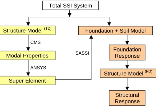
Figure 2 shows a flow diagram for CMS-based SSI analysis by SASSI.
Fig 2 – Flow Diagram of CMS-Based SSI Analysis
The analysis steps are described below:
1. Partition the structure into its components. In general, the physical characteristics of the structure are used to select suitable components. The components should also be defined so as to minimize the number of interfaces between them. This will significantly reduce computer run time.
2. Construct the normalized displacement modes for each component that includes the constrained interface and
normal modes. The internal displacements of components are represented in generalized coordinates with selected number of modes while the boundary displacements are represented in global DOF’s for ease of coupling of components through standard finite element direct stiffness assembly.
3. Compute the component mass and stiffness matrices following the CMS formulations in Eq. 14. These matrices
are also referred to as super-element matrices.
4. Compute component damping matrices; e.g. using the procedure presented in Eq. 19.
5. Incorporate super-element mass, stiffness and damping matrices in the foundation model represented by
foundation dynamic impedance and scattered motions and solve the equation of motion to determine the component boundary and foundation dynamic responses.
6. Using the component boundary and foundation dynamic responses, calculate the response of each component.
Steps 1 through 3 can be readily carried out in commercial computer programs such as ANSYS®. The computer program MTR/SASSI® is used to carry out steps 4, 5 and 6.
VALIDATION
In order to check out the procedure outlined above, the frequency response of a lumped mass parameter model with mass eccentricity supported on a square mat foundation on uniform halfspace is examined (see Fig. 3). The dynamic properties of the structure, foundation basemat and soil media are summarized below. The model is subjected separately to vertical and horizontal excitation by respectively applying vertically propagating harmonic P- and SV-waves with control motion specified at the free-field ground surface.
Total SSI System
Structure Model (TD) Foundation + Soil Model
(FD)
Modal Properties
Super Element
CMS
ANSYS
Foundation Response
SASSI
Structure Model (FD)
Beam Properties: Mat Properties: Halfspace Properties:
E = 2.4*1012 N/m2 L = W = 28.0 m Vs = 600 m/s
Poisson’s Ratio = 0.3 E = 1.0*1012 N/m2 Vp = 2,000 m/s
Density = 0. Thickness = 1.0 m Density = 1,300 Kg/m3
Section Area = 0.15 m2 Poisson’s Ratio = 0.333 Damping Ratio = 0.
Ixx = Iyy = 0.50 m4 Density = 2,950 Kg/m3
Damping Ratio = 0.02
Fig 3 – Lumped Mass Parameter SSI Model
X Y
Z
X Y
Z Component Model Foundation + Super Element
SE SE
Structural Analysis Super Element
Foundation Motion
84
82 84
82
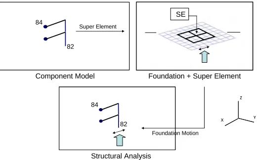
Fig 4 – CMS-Based SSI Analysis Steps
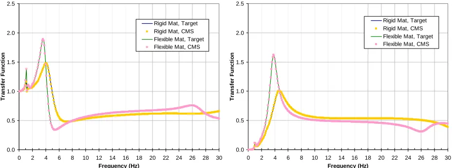
The total SSI system was first analyzed in frequency domain using SASSI to obtain the baseline solution. Two cases of rigid and flexible basemats were analyzed. Figure 5 and 6 show the x and y transfer function (TF) response of rigid and flexible foundation basemat (Node 82) from x-excitation, respectively. Similar TF results at top mass node (Node 84) are shown in Figs. 7 and 8, respectively. For the vertical excitation, the foundation and top mass node responses in the x any y directions are shown in Figs. 9 and 10, and Figs. 11 and 12, respectively. The TF responses in the y direction due to z-excitation are the same as those of the x-direction due to symmetry and, therefore, are not shown.
Following the calculation of baseline responses above, the structural model was partitioned from the total system and modeled as CMS component. The component modal mass and stiffness matrices were then calculated from ANSYS® and incorporated into the foundation model as element. Figure 4 shows the CMS partitioning scheme. The combined super-element structural component and foundation model were then analyzed by SASSI to compute the foundation response (Node 82). The foundation responses were then back-substituted into the structural component and analyzed by SASSI to calculate the structure response.
M1 = 1.3E7 Kg
M2 = 3.4E7 Kg 84
83
82
X Y
Z Rigid Links
3 m
0.0 0.5 1.0 1.5 2.0 2.5
0 2 4 6 8 10 12 14 16 18 20 22 24 26 28 30 Frequency (Hz) T ran sf e r Fu nc ti on
Rigid Mat, Target Rigid Mat, CMS Flexible Mat, Target Flexible Mat, CMS
0.0 0.5 1.0 1.5 2.0 2.5
0 2 4 6 8 10 12 14 16 18 20 22 24 26 28 30 Frequency (Hz) T ran s fer Fu nc ti on
Rigid Mat, Target Rigid Mat, CMS Flexible Mat, Target Flexible Mat, CMS
Fig 5 – X-Response Due to X-Input, Node 82 Fig 6 – Y-Response Due to X-Input, Node 82
0.0 0.5 1.0 1.5 2.0 2.5
0 2 4 6 8 10 12 14 16 18 20 22 24 26 28 30 Frequency (Hz) T ran sf er Fu nct ion
Rigid Mat, Target Rigid Mat, CMS Flexible Mat, Target Flexible Mat, CMS
0.0 0.5 1.0 1.5 2.0 2.5
0 2 4 6 8 10 12 14 16 18 20 22 24 26 28 30 Frequency (Hz) Tr ans fer Funct ion
Rigid Mat, Target Rigid Mat, CMS Flexible Mat, Target Flexible Mat, CMS
Fig 7 – X-Response Due to X-Input, Node 84 Fig 8 – Y-Response Due to X-Input, Node 84
0.0 0.1 0.2 0.3 0.4 0.5 0.6 0.7
0 2 4 6 8 10 12 14 16 18 20 22 24 26 28 30 Frequency (Hz) Tr ansf er Funct ion
Rigid Mat, Target Rigid Mat, CMS Flexible Mat, Target Flexible Mat, FIM
0.0 0.2 0.4 0.6 0.8 1.0 1.2 1.4 1.6 1.8
0 2 4 6 8 10 12 14 16 18 20 22 24 26 28 30 Frequency (Hz) Tr ansf er Funct ion
Rigid Mat, Target Rigid Mat, CMS Flexible Mat, Target Flexible Mat, CMS
0.0 1.0 2.0 3.0 4.0 5.0 6.0
0 2 4 6 8 10 12 14 16 18 20 22 24 26 28 30 Frequency (Hz)
T
ran
sf
e
r Fu
nc
ti
on
Rigid Mat, Target Rigid Mat, CMS Flexible Mat, Target Flexible Mat, CMS
0.0 0.5 1.0 1.5 2.0 2.5 3.0
0 2 4 6 8 10 12 14 16 18 20 22 24 26 28 30 Frequency (Hz)
T
ran
sf
e
r Fu
nc
ti
on
Rigid Mat, Target Rigid Mat, CMS Flexible Mat, Target Flexible Mat, CMS
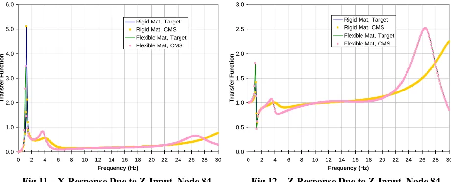
Fig 11 – X-Response Due to Z-Input, Node 84 Fig 12 – Z-Response Due to Z-Input, Node 84
The TF results of the SSI analyses using component modes are compared with the baseline (target) results in Figs. 5 through 12 for both the rigid and flexible foundation basemats. As seen from these figures, there is excellent agreement between the one-step analysis results and those obtained utilizing CMS method.
SUMMARY AND CONCLUSIONS
Method of component mode synthesis (CMS) of large structural systems based on fixed-interface natural modes and interface constrained modes (including rigid body modes) properties of the components were presented. The method was then applied to seismic SSI formulation using sub-structuring method. It was shown that by suitable selection of structural components and reduced number of kept-normal modes, the size of the global reduced SSI model to be solved can be made small and manageable. Once the foundation and component interface responses are calculated, they can be back-substituted in each component model to determine the final response of the structure. The accuracy of the procedure was checked out using an example of a lumped parameter model with mass eccentricity supported on rigid and flexible basemats on uniform soil media. The SSI response of this model calculated using one-step approach by SASSI and CMS-based SSI approach by
ANSYS® and SASSI shows excellent agreement. Because the CMS method is well established and widely used, it is
expected that very large and complex SSI systems with multi-million degrees of freedom in the structure can be analyzed utilizing this method.
REFERENCES
1. Lysmer, J., Tabatabaie, M., Tajirian, F., Vahdani, S. and Ostadan, F., “SASSI – A System for Analysis of Soil Structure Interaction,” Report No. UCB/GT/81-02, Geotechnical Engineering, Department of Civil Engineering, University of California, Berkeley, 1981.
2. MTR/SASSI®, 2009. System for Analysis of Soil-Structure Interaction, Version 8.0, Volume I User’s Manual, MTR & Associates, Inc., Lafayette, California, United States.
3. ANSYS®, a general-purpose finite element analysis (FEA) software. ANSYS, Inc., Southpointe 275 Technology Drive, Canonsburg, PA 15317, United States.
4. Hurty, W.C., “Vibrations of Structures by Component Mode Synthesis,” Proceedings Am. Soc. Civil Engrs, J. Eng. Mech., Div. 86, August 1960.
5. Hurty, W.C., “Dynamic Analysis of Structural Systems by Component Mode Synthesis, “Jet Propulsion Lab, California Institute of Technology TR 32-530, 1964.
6. Craig, R.R. Jr. and Bampton, M.C., “Coupling of Substructures for Dynamic Analyses,” AIAA Journal, 1968. 7. Craig, R.R., “Coupling of Substructures for Dynamic Analyses: An Overview, AIAA Journal, 2000.
8. Craig, R. R. Jr., “A Review of Time Domain and Frequency Domain Mode Synthesis Methods,” Modal Analysis, 1987. 9. Gladwell, G.M.L., “Branch Mode Analysis of Vibrating Systems,” J. Sound Vib., 1964.
10. Rubin, S., “Improved Component-Mode Representation for Structural Dynamic Analysis,” AIAA Journal, 1975. 11. Balmes, E., “Use of Generalized Interface Degrees of Freedom in Component Mode Synthesis,” Proceedings of