ABSTRACT
MISKIEWICZ, MATTHEW NILE. Computer Generated Geometric Phase Holograms. (Under the direction of Michael Escuti.)
This dissertation concerns the fabrication, analysis, and simulation of computer generated geometric phase holograms (CGHs). The current knowledge of CGHs is advanced to enable the creation of new sophisticated optical elements with unique characteristics. These elements enable new technologies related to displays, astronomy, sensing, beam-steering, beam-shaping, and more.
First, a novel direct-write system for CGH creation is presented. A mathematical description of the system is developed which allows the result of a given scan pattern to be predicted. The accuracy of the model is validated with various scan patterns, then a high-quality direct-write polarization grating and q-plate are fabricated for the first time.
With a system capable of creating CGHs, the most common and useful CGHs are explored in depth: the polarization grating, the geometric phase lens, and the Fourier geometric phase hologram. For each element, the possible scan patterns and parameters and their effect on the resulting element’s quality are studied. Ultimately, the optimal scan patterns and parameters are found, then best-quality elements of each type are created and characterized.
© Copyright 2014 by Matthew Nile Miskiewicz
Computer Generated Geometric Phase Holograms
by
Matthew Nile Miskiewicz
A dissertation submitted to the Graduate Faculty of North Carolina State University
in partial fulfillment of the requirements for the Degree of
Doctor of Philosophy
Electrical Engineering
Raleigh, North Carolina
2014
APPROVED BY:
John Muth Michael Kudenov
Russell Philbrick Michael Escuti
BIOGRAPHY
Matthew Miskiewicz was born and raised in Clearwater Florida. After moving to North Car-olina, he attended Wake Technical Community College for a semester before joining North Carolina State University (NCSU). Initially enrolled in civil engineering, he switched to elec-trical and computer engineering (ECE) where he stayed for the remainder of his collegiate education.
ACKNOWLEDGEMENTS
TABLE OF CONTENTS
LIST OF TABLES . . . v
LIST OF FIGURES . . . vi
Chapter 1 Introduction . . . 1
1.1 Light in Everyday Life . . . 1
1.2 Geometric Phase Holograms . . . 2
1.3 Dissertation Structure . . . 3
1.4 Publications From This Work . . . 4
Chapter 2 Background. . . 6
2.1 Geometric Phase Holograms . . . 6
2.1.1 Geometric Phase . . . 6
2.1.2 Summary of Important GPH Concepts . . . 10
2.1.3 Polarization Grating . . . 10
2.1.4 GPH Fabrication Techniques . . . 11
2.2 Liquid Crystals . . . 12
2.2.1 Physical Properties of Liquid Crystals . . . 12
2.2.2 Alignment of Liquid Crystals . . . 15
2.2.3 Fabrication of LC Films . . . 16
2.3 Electromagnetic Waves . . . 17
2.3.1 The Electromagnetic Wave Equations . . . 17
2.3.2 Infinite Plane Wave Solution . . . 18
2.3.3 Diffraction . . . 19
2.3.4 General Solution . . . 19
2.4 Electromagnetic Finite-Difference Time-Domain Simulation . . . 20
2.4.1 Mathematical Basis . . . 21
2.4.2 The Yee Cell . . . 22
2.4.3 FDTD Summary . . . 23
Chapter 3 Direct Write System for CGH Creation. . . 24
3.1 Introduction . . . 24
3.2 System Design . . . 25
3.3 System Description . . . 27
3.3.1 Approach . . . 27
3.3.2 System Inputs and Electromagnetic Output . . . 28
3.3.3 Adjusted Electromagnetic Output . . . 28
3.3.4 LC Response . . . 30
3.3.5 Physical Interpretation ofH and T . . . 31
3.4 System Description Validation . . . 31
3.4.1 Fluence Threshold . . . 33
3.4.2 DOLP Threshold . . . 34
3.5 Analysis of Selected Scan Patterns . . . 35
3.5.1 Adjacent Scan Lines . . . 35
3.5.2 Intersecting Scan Lines . . . 36
3.5.3 Q-Plate . . . 39
3.5.4 Polarization Grating . . . 41
3.6 Conclusion . . . 41
Chapter 4 Computer Generated Polarization Gratings . . . 43
4.1 Polarization Gratings . . . 43
4.2 Scan Pattern and Parameters . . . 45
4.3 Scan Pattern Optimization . . . 46
4.3.1 Scan Pattern Evaluation Strategy . . . 46
4.4 Parameter Space Analysis . . . 48
4.5 Experimental Results . . . 50
4.6 Analysis of Non-Ideal PG Diffraction . . . 51
4.6.1 Incorrect Retardation . . . 52
4.6.2 LC Defects . . . 53
4.6.3 Nonlinear Phase Profiles . . . 54
4.6.4 Non-Ideal PG Diffraction Summary . . . 58
4.7 Highest-Quality Direct-Write Fabricated PG . . . 59
4.8 Conclusions . . . 60
Chapter 5 Computer Generated Geometric Phase Lenses . . . 61
5.1 GPL Phase Profile . . . 62
5.1.1 Ideal GPL Profile . . . 62
5.1.2 Parabolic And Spheric Approximations . . . 63
5.2 Scan Pattern and Parameters . . . 65
5.2.1 Linear Archimedean Spiral . . . 65
5.2.2 Nonlinear Archimedean Spiral . . . 67
5.3 Spiral Sampling . . . 67
5.3.1 Uniform Time Sampling . . . 68
5.3.2 Uniform Arc Length Sampling . . . 69
5.3.3 Uniform Angular Distance Sampling . . . 69
5.4 Spiral Sampling Comparison . . . 70
5.5 Parameter Space Analysis . . . 72
5.5.1 Orientation Profile and Alignment Quality . . . 72
5.5.2 Comparison of Lens Operation . . . 72
5.6 Characterization of Highest Quality GPL . . . 76
5.7 Conclusions . . . 77
Chapter 6 Fourier Geometric Phase Holograms . . . 78
6.1 Ideal FGPH Behavior . . . 78
6.2 FGPH Scan Pattern . . . 80
6.3 Theoretical Impact of Beam Size . . . 82
6.3.2 Small Beam Size . . . 83
6.4 Experimental Results . . . 84
6.4.1 LC Alignment Quality and Profile Observations . . . 84
6.4.2 FGPH Reconstruction Comparison . . . 84
6.4.3 Characterization of High-Quality FGPH . . . 88
6.5 Conclusions . . . 89
Chapter 7 Electromagnetic Simulation of CGH . . . 91
7.1 Algorithm Derivation . . . 92
7.1.1 Source Definition . . . 92
7.1.2 Update Equations . . . 94
7.2 Near-to-Far-Field Transformation . . . 96
7.2.1 Far-Field Wavevector . . . 96
7.2.2 Far-Field Polarization . . . 97
7.3 Algorithm Validation . . . 98
7.3.1 Glass Etalon . . . 98
7.3.2 Crossed Polarizer Pair . . . 99
7.3.3 Twisted Nematic Cell . . . 99
7.3.4 Bragg Grating . . . 101
7.3.5 Photonic Band Gap Structure . . . 102
7.3.6 2D Array of Conducting Particles . . . 103
7.3.7 2D Asymmetric Grating . . . 104
7.4 GPH Simulation . . . 104
7.4.1 GPH Multiple Beam Splitter . . . 105
7.4.2 GPH Micro Lens Array . . . 109
7.5 Summary and Conclusions . . . 112
Chapter 8 Conclusion . . . .113
8.1 Direct-Write System for CGH Creation . . . 113
8.2 Study and Optimization of CGHs . . . 113
8.3 FDTD for Simulation of CGHs and GPHs . . . 114
8.4 Future Research Directions . . . 115
8.5 Closing . . . 115
References. . . .117
Appendices . . . .124
Appendix A Geometric Phase via a Birefringent Retarder . . . 125
Appendix B Wavelength Dependence of Dynamic Phase Elements vs. GPH . . . 127
Appendix C Complex Phase Accuracy: A General, Quantitative GPH Metric . . . . 129
C.1 Complex Phase and GPHs . . . 129
LIST OF TABLES
Table 4.1 Summary of PG non-idealities (top) and corresponding causes (left). . . 59 Table 4.2 Summary of the deduced causes of non-idealities in fabricated samples. . . 59
Table 5.1 Scan parameters used for fabricated lenses. . . 72
LIST OF FIGURES
Figure 1.1 Images of various GPHs made possible by this dissertation. These elements enabled new technologies related to astronomy, displays, and sensing. . . 2
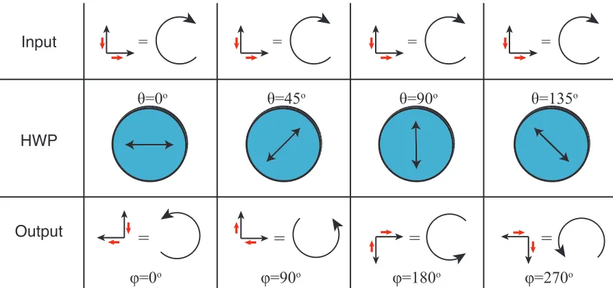
Figure 2.1 Geometric phase via. a birefringent retarder. The input and output polar-ization is shown in the form of an orthogonal vector sum (the red arrow indicates the phase of each component) and also in standard circular po-larization notation. The half-wave plate (HWP) has a dynamic phase term that is modulo 2π. The accumulated geometric phase φis equal to twice the orientation angle θ. . . 9 Figure 2.2 The NCSU mascot in various polarization states images directly (a,d) and
through a PG (b,c,e,f). . . 11 Figure 2.3 a) Example rod-like LC molecule and anisotropy in index of refraction. b)
LC in the nematic phase. c) A macro-scale analog to LCs, matchsticks in a box exhibit partial order. . . 13 Figure 2.4 Cross section of LC films fabricated in this dissertation. . . 17 Figure 2.5 Fields propagating through a PG; red and blue colors indicates positive and
negative fields respectively. This result was obtained using a version of the FDTD method developed in this work (see Chap. 7) and is extremely difficult if not impossible to obtain with analytic methods. . . 21 Figure 2.6 The grid scheme used in this work is the 3D Yee grid; shown is a unit cell
with the location of theE and Hfields). . . 22
Figure 3.1 High-level schematic of the kind of polarization direct-write system studied in this paper. . . 26 Figure 3.2 High-level view of our direct-write system description, which starts with the
system inputs and ends with the LC response. The transformation functions H and T relate to material properties of the LPP and LC respectively; all other operations are purely mathematical and make no assumptions about material properties. . . 27 Figure 3.3 Graphical representation of some properties of our chosen H, which takes
the average of all input Stokes vectors. Each diagram is a 2D cross-section of the Poincare sphere (since we are only concerned with linear polariza-tion), and the ring in each diagram represents a DOLP of 1. a) Non-causality and orientation averaging. b) Depolarization by superposition of orthogonal polarizations. . . 29 Figure 3.4 Threshold functions used to predict the magnitude of the LC anchoring vector
Figure 3.5 a) Polarizing optical microscope setup used to capture the images in this paper. The Full-Wave Plate (FWP) is used to distinguish between 0◦ and 90◦ polarized light. b) The full-color colormap for differently aligned liquid crystals, acquired when using the FWP. c) The grayscale colormap acquired without the FWP (0◦ and 90◦ are indistinguishable). Orientation angle pro-files of films were measured by matching the film’s color with b) using the least squares algorithm. . . 32 Figure 3.6 The first validation experiment, designed to test the effect of fluence on LC
alignment. Pattern a) was created by scanning adjacent, uniform vertical lines and varying the fluence in the horizontal dimension. Pattern c) is the reverse of pattern a), and pattern b) is the superposition of a) and c). From this experiment we determined a fluence threshold to be used in subsequent simulations. . . 33 Figure 3.7 The second validation experiment, designed to test 1) the effect of DOLP on
LC alignment quality, and 2) if the LC aligns to the average exposure angle of the LPP. Pattern a) was created by scanning adjacent, uniform vertical lines and varying the polarization angle in the horizontal dimension from 0◦ to 90◦. Pattern c) is the same as a), except the polarization varies from 0◦ to -90◦. Pattern b) is the superposition of a) and c) with half fluence each (equivalent total fluence). From this experiment we determine a DOLP threshold to be used in subsequent simulations and confirm the aligning properties of the LC. 35 Figure 3.8 Adjacent, uniform scan lines with polarization orientations of ψ0−50◦,ψ0◦,
andψ0+50◦. The distance between the scan lines decreases from a) to c), and
we observe an averaging of the LC orientation angle. By sufficiently overlap-ping neighboring scan lines, we can create continuously varying orientation profiles. . . 37 Figure 3.9 Two intersecting scan lines with polarization orientations 0◦ and 90◦. The
average polarization angle at every location is either 0◦, 90◦, or undefined where the fluence delivered by each line is equal. As a result, discrete domains are produced. a) Simulated F, b) Davg, c) |A|, d) ψavg using the color bar in Fig. ??(b), e) A, created by overlaying c) and d). f) Actual image of fabricated film, color bar in Fig. ??(b). . . 38 Figure 3.10 A simulated and fabricated q-plate, which is a kind of azimuthal waveplate.
a) SimulatedF, b)Davg, c)|A|, d)ψavg using the color bar in Fig.??(b), e)
A, created by overlaying c) and d). f) Actual image of fabricated film, color bar in Fig. ??(b). . . 39 Figure 3.11 A PG fabricated by scanning adjacent scan lines, where the polarization
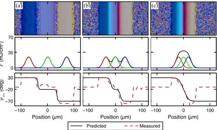
rotates from line to line. The target PG pitch is 50 µm and the scan lines were spaced 7 µm apart using a beam width of 7.5 µm. a), b), and c) are images obtained using different magnification objective lenses and the plots below show the desired orientation profile compared to our measured profile. 40
Figure 4.2 Simulated results for a scan pattern with B = 0.6, L= 0.4, andFave = 200 mJ/cm2. a) Intensity cross section for each scan line influencing a single
pitch. b) Total fluence. c) Average degree of linear polarization (DOLP). d) Alignment quality calculated using b) and c). e) Phase profile, found as twice the LC orientation angle. f) Diffraction efficiencies found by applying the NTFFT on e). From the results, we can evaluate these scan parameters as unfavorable. . . 47 Figure 4.3 Simulated results for a scan pattern with B = 0.8, L= 0.2, andFave = 200
mJ/cm2. a) Intensity cross section for each scan line influencing a single pitch. b) Total fluence. c) Average degree of linear polarization (DOLP). d) Alignment quality calculated using b) and c). e) Phase profile, found as twice the LC orientation angle. f) Diffraction efficiencies found by applying the NTFFT on e). From the results, we can evaluate these scan parameters as favorable. . . 48 Figure 4.4 The predicted alignment quality|A|vs. the normalize beam size B and the
normalized line spacing L. Poor alignment quality results in LC defects, in-correct retardation, and inin-correct alignment orientation; all of these things reduce η+1. . . 49
Figure 4.5 The predictedη+1|A|vs. the normalize beam sizeB and the normalized line
spacingLassuming|A|= 1. These efficiencies assume the profile is perfectly aligned and so represent an upper limit. . . 50 Figure 4.6 Predicted optimal scan parameters for creating high-efficiency PGs.
Param-eters inside the white triangular region have high efficiency. ParamParam-eters with larger line spacing result in a shorter scan time. Parameters farther from the edges of the high-efficiency region have the maximum yield, i.e., the highest likelihood of success. . . 51 Figure 4.7 Polarizing microscope images of fabricated samples. Different shades
corre-spond to different alignment orientations. Samples g and h represent high-quality alignment. . . 52 Figure 4.8 Images of a 633 nm beam after passing through samples A-I. Samples d, e, g,
and h are the highest quality of the nine samples, but there still significant power diffracted into the 0 and +2 orders; since the alignment quality is good, this indicates the alignment profiles are nonlinear. Samples a and b show many other higher orders, indicating these profile are very nonlinear. The background noise in samples c, f, and i is caused by the massive quantity of LC defects which scatter the incident beam and greatly reduce the efficiency. 53 Figure 4.9 a-b) Examples of super-grating profiles. c-d) The simulated η+1 associated
Figure 4.10 a) Examples of noisy PG phase profiles. b) Simulated η+1 vs. noise level.
c-d) Simulated diffraction efficiencies of noisy phase profiles (pure noise, no linear PG profiles). Noise in the phase profile results in diffraction into all directions, similarly to scattering. . . 56 Figure 4.11 a) Examples of sawtooth-grating profiles. b) Simulatedη+1vs. the scale factor
ξ. c-d) The simulated D.E.s associated with the profiles in a). The sawtooth-grating profile is characterized by a linear phase with a slope of 2πξ/Λ. The sawtooth profile may be caused by errors in the direct-writing system or LC fabrication errors, and the profile results in power directed into orders other than +1. . . 58 Figure 4.12 Very high quality direct-write fabricated PG with a pitch of 30 µm and
η+1 > 99.7%. a) Polarizing microscope image of the sample. b) Image of a
633 nm laser after diffracting through the sample. . . 60
Figure 5.1 Demonstration of the polarization properties of a GPL. Different circular polarizations converge or diverge; unpolarized light is equivalent to linearly polarized light and acts as the superposition of both circular polarizations. . 62 Figure 5.2 Comparison of the ideal lens profile, parabolic approximation, and spheric
approximation. The lens f-number is a) 5, b) 2.5, and c) 0.5. The parabolic profile is a good approximation when the f-number is high, and only at low f-number does the profile differ significantly from the ideal. The spherical approximation is only good at high f-number. . . 64 Figure 5.3 a) Linear Archimedean spiral. b) Nonlinear Archimedean spiral. The
nonlin-ear spiral is more efficient in terms of scan time, but can only be used if the beam size can be changed dynamically, as in our system. . . 66 Figure 5.4 The spiral pattern sampled with a) uniform time, b) uniform arc length, and
c) uniform angular distance. The sampled points are assumed to be connected by straight lines. A key observation is that sampled points of adjacent lines in a) and b) are misaligned to each other, but sampled points of adjacent lines in c) are aligned to each other. . . 68 Figure 5.5 Polarizing microscope images of fabricated GPLs. a) Uniform arc length
sam-pling withd0 = 200µm. b) Uniform arc length sampling with d0 = 100µm.
c) Uniform angular distance sampling with θ0 = 2π/50. c) Uniform angular
distance sampling withθ0= 2π/200. . . 71
Figure 5.6 Polarizing microscope images of samples A-D. Sample A and B both show very good alignment. Sample C suffers from a staircase profile. Sample D has many LC defects, except for the center of the pattern where the beam size could not be increased any further and soB was lowered. . . 73 Figure 5.7 High-magnification polarizing microscope images of the edge of samples A-D.
Here the phase profile and defects can be seen more clearly. . . 74 Figure 5.8 Images of the fabricated GPLs in operation. A 633 nm laser was sent through
Figure 5.9 Measured cross section of a 633 nm laser a) without alteration, b) after GPL with RCP input, c) after GPL with LCP input. . . 76
Figure 6.1 a) Target FGPH image used in this section. b) Needed phase profile calculated for the Gerchberg-Saxton algorithm. c) Predicted reconstructed image for RCP input. d) Predicted reconstructed image for LCP input. . . 79 Figure 6.2 Scan pattern used to record FGPHs. . . 81 Figure 6.3 Example target and actual exposure polarizations when using a Pockels cell;
the polarization is blurred between between each polarization state. This example assumes a pixel pitch of 10µm and that a polarization modulation takes 1µm to finish. . . 82 Figure 6.4 Polarizing microscope images with various zoom of fabricated FPGH with
the target phase profile shown in Fig.??(b). All samples had the same scan pattern parameters, except for the beam size, which varied from 10µm (B = 0.5) to 43µm (B = 2.2). When the beam size is smaller, the pixels are more clearly defined. When the beam size is larger, more averaging takes place. Extremes at either end cause many LC defects; a beam size of ∼ B = 1 seems optimal. . . 85 Figure 6.5 The FGPH characterization setup. A 633 nm laser passes through an iris to
clean up the beam, a polarizer to control beam power and ensure polariza-tion purity, a quarter-wave plate (QWP) to set the polarizapolariza-tion, the FGPH element, and a series of lenses which focus the image onto a CCD. . . 86 Figure 6.6 The Fourier images produced by FGPHs with various beam sizes. Polarizing
microscope images of the FGPHs are in Fig.??, and the setup used to capture these images is in Fig.??. . . 87 Figure 6.7 Images produced by sample B (B = 1.1) with both a 633 nm and 523 nm
laser. Images were acquired using a beam-splitter and multiple QWPs to set beam polarizations. The green image is a smaller scaled version of the red image. a) RCP red and LCP green. b) RCP red and RCP green. . . 89
Figure 7.1 (a)) The simulate space used for Wolfsim 3D. b) The grid scheme used in this work is the 3D Yee grid; shown is a unit cell with the location of the E
and Hfields (which are identical to the positions of thePand Q fields). . . . 93 Figure 7.2 Comparison of possible diffraction orders of an arbitrary 2D periodic
struc-ture in a) k-space, and b) real space. This figure demonstrates conical diffrac-tion. . . 97 Figure 7.3 a) A glass etalon with index n= 1.5 and thickness dsurrounded by air. b)
Simulated (circles) and analytic (dashed/solid) transmission. The source was incident at{θ= 40◦,φ= 90◦}. . . 99 Figure 7.4 Conoscopic contour plot of the transmission through a pair of crossed dichroic
polarizers. a) Our result. b) Berreman 4x4 result. Contour lines start at 0.001 (centermost) and increase in steps of 0.005. . . 100 Figure 7.5 FDTD simulation results for an LC cell between crossed polarizers compared
Figure 7.6 a) A Bragg grating with d = 5 µm, Λ = 0.45 µm, 1 = 2.2525, 2 = 0.15,
andσ1=σ2= 250 S/m. b) The simulated transmission of the m=−1 order
using Wolfsim 3D and RCWA (dashed). For each case, the source was TE and incident atθ= 37.67◦. . . 102 Figure 7.7 a) A photonic band gap structure with a = 9 mm, d = 4 mm, and r =
4.2. Solid lines are our results, dashed lines are results from [61]. b) The transmission coefficient for the incidence directions indicated. The source was TM polarized for the oblique cases and polarized in the y direction for the normally incident case. . . 103 Figure 7.8 a) The geometry of the infinite 2D array of square perfect electric conductor
particles. b) Reflectance through the 2D arrary. Inset: a close up of the 100% reflectance maxima for normal incidence andφ= 45◦ and θ= 5◦. . . 104 Figure 7.9 a) Structure of the simulated 2D grating. b) Far-Field orders resulting from
Wolfsim 3D and an RCWA code for an x-polarized linear input. . . 105 Figure 7.10 a) Target k-space image for anM = 5 MBS. Orders have equal intensity but
unspecified phase. b) A calculated possibly optimal phase profile to produce this k-space image. . . 106 Figure 7.11 Analytic and simulated k-space images (far-field orders) resulting from the
MBS profile given in Fig.??(b) and Λ = 5µm. Analytic output with a) RCP, and b) linear (all linear polarizations are the same). FDTD simulated output with input a) RCP, b) 0◦ linear, c) 45◦, and d) 90◦. . . 107 Figure 7.12 Simulated k-space images (far-field orders) resulting from the MBS profile
given in Fig. ??(b) and Λ = 10 µm. FDTD simulated output with input a) 0◦ linear, b) 45◦, and c) 90◦. These results match the analytic results closer than when Λ = 5 µm. . . 108 Figure 7.13 Polarizing microscope image of a GP MLA made with The Howlographer.
Image courtesy Jihwan Kim. . . 109 Figure 7.14 a) Unit cell of the target MLA phase profile. Simulated phase profile of 550
nm light directly after the MLA for b)Ex fields, c)Ey fields, and d)Ezfields. These are the inputs to the vacuum wave propagation algorithm. . . 110 Figure 7.15 Calculated total field power after the MLA forxz andyz cross sections. The
Chapter 1
Introduction
1.1
Light in Everyday Life
The ability to control light is a cornerstone of 21st century society. We use incandescent bulbs, fluorescent bulbs, and LEDs to light schools, office buildings, and sports fields. Liquid crystal displays are present in mobile smartphones, desktop monitors, gas station pumps, cash registers, clocks, and countless other devices. Eyeglasses and contact lenses allow millions of people to see the world more clearly. Lasers are used in fiber optic and telecommunication technology giving us high-speed internet, as well as being foundational to basics science research. Cameras allow us to capture and preserve images and scenes, while optical disc readers and projectors allow us to replay scenes to a wide audience.
We are continuing to realize things that were once science fiction, such as 3D holograms, laser weapon systems, and coin-sized projectors. However, these and other technologies and end-products are the result of decades of fundamental research by the scientific community into the generation and manipulation of light. These researchers include optical scientists, physicists, astronomers, electrical engineers, computer engineers, material engineers, and others who have explored the basic phenomena surrounding electromagnetic waves and their interaction with physical media.
Vector Apodizing
Phase Plate Polarization Grating Fourier Hologram
Figure 1.1: Images of various GPHs made possible by this dissertation. These elements enabled new technologies related to astronomy, displays, and sensing.
1.2
Geometric Phase Holograms
So what is this amazing GPH element? First and foremost, it is a hologram...but what exactly is that? One definition of a hologram is an optical element with a higher information density than a photograph. For example, when you take a picture of a bed of flowers, you are storing information about the scene from a single perspective with a single focus. With a hologram, you can store information about the scene from multiple perspectives (i.e., multiple viewing angles) and/or multiple focuses (i.e., focusing on the foreground, the flowers, or the background) all in a single element. This property of high information density means that holograms have many uses that extend beyond 3D intergalactic communication with Darth Vader. Perhaps the most successful commercial use of holograms is extremely fast and compact encrypted data storage [5].
There are many technologies for recording and replaying holograms and each has a different physical operating principle. GPHs use something called the geometric phase of light to record and replay information about a scene. Use of the geometric phase gives GPHs their unique and advantages features. These features are summarized as follows:
• Superior optical characteristics when compared with other holograms
• Fabrication using low-cost commercial materials
• Ability to manipulate polarized light
• Ability to respond to different wavelengths of light (i.e., different colors) in a controlled manner
This dissertation focuses on a specific class of GPHs: Computer Generated Geometric Phase Holograms (CGHs); computer generated in the sense that a computer controls the generation and fabrication of the hologram. Going back to the example of the flower bed, one might take sophisticated and expensive equipment to the actual flower bed to record a GPH of the scene. Or, a computer could be used to simulate the geometry, lighting, and color of the flower bed and calculate the hologram that would be recorded from the scene; then use a holographic printer to turn this calculated hologram into an actual element. The later demonstrates the core concept of the CGH, although none of the CGHs studied and created in this dissertation are as complex as this.
1.3
Dissertation Structure
Chapter 2 contains technical background information to equip the reader with the knowledge and terminology needed for the proceeding chapters. The topical coverage begins with the fundamentals of geometric phase and GPHs. Next, the key properties of liquid crystals are discussed and the fabrication processes used in this dissertation are described. The concept of diffraction is introduced and various solutions for the general diffraction problem are discussed. Finally, the electromagnetic finite-difference time-domain (FDTD) method is reviewed.
In Chapter 3, we1 address the following questions:What system configuration will en-able the recording of arbitrary CGHs with quality well beyond the prior art? What mathematical system description will allow us to accurately model the system? To answer these questions, we study a new tool, called The Howlographer, for CGH fabrication using a direct-write laser system, photoalignment polymers, and liquid crystals. We lay out a thorough mathematical description of the system that allows us to predict the physical prop-erties of fabricated CGHs based on system inputs. After verifying the accuracy of the system description, we use it to fabricate and study several interesting patterns. The primary contribu-tion of this chapter is the design, system descripcontribu-tion, and validacontribu-tion of a new direct-write system that is the first tool capable of creating arbitrary CGHs with continuously varying profiles.
In Chapters 4, 5, and 6, we address the following questions:What are design parameters for fabricating important CGH elements, and what impact do these parameters have on the element’s properties? What are the optimal parameters for fabricating the highest quality CGHs? To this end, we design, fabricate, and study the most important CGH elements: polarization gratings, geometric phase lenses, and arbitrary Fourier GPHs. For each element, we study the various system inputs that can be used to generate the element
1
and use our system description to predict the advantages and disadvantages of each. Then we fabricate many elements using a wide range of input parameters, and characterize them with metrics such as diffraction efficiency, zero-order leakage, scattering efficiency, and polarization contrast. The primary contribution of these chapters is the creation and characterization of the first high quality CGH polarization gratings, geometric phase lenses, and arbitrary Fourier GPH, and the determination of the optimal parameters for fabricating these elements.
In Chapter 7, we address the following question: What numerical simulation tool is ideal for simulating the physical phenomena present in GPHs? Seeing no such tool in prior art, we develop a new algorithm based on the FDTD algorithm, a popular method based on Maxwell’s equations. We derive the key mathematical equations of the algorithm, validate its accuracy and ability to simulate GPHs, and simulate for the first time several GPHs. The tool is open source and available online [6]. The primary contribution of this chapter is the creation of the first tool capable of simulating arbitrary, 3D, anisotropic structures that are periodic in two dimensions with sources incident from anywhere in the hemisphere (conductive materials are supported as well).
1.4
Publications From This Work
Published Refereed Journal Manuscripts
1. M. N. Miskiewicz, S. Stefan, and M. J. Escuti. An FDTD algorithm for whole-hemisphere incidence on 2D periodic media. IEEE Trans. on Atenn. and Prop. 2014. 62(3), pp. 1348-1353. 2014
2. M. W. Kudenov, M. N. Miskiewicz, M. J. Escuti and E. L. Dereniak. Spatial heterodyne interferometry with polarization gratings. Opt. Lett. 37(21), pp. 4413-4415. 2012.
In Press Refereed Journal Manuscripts
1. M. N. Miskiewicz and M. J. Escuti. Direct-writing of complex liquid crystal patterns. Opt. Express. 2014.
2. M. W. Kudenov, M. N. Miskiewicz, and M. J. Escuti. Polarization Spatial Heterodyne Interferometer: Model and Calibration. Opt. Eng. 2014.
Published Refereed Conference Proceedings
Modern Technologies in Space-and Ground-Based Telescopes and Instrumentation II. pp. 8450. 2012.
2. M. N. Miskiewicz, J. Kim, Y. Li, R. K. Komanduri and M. J. Escuti. Progress on large-area polarization grating fabrication. Acquisition, Tracking, Pointing, and Laser Systems Technologies XXVI. pp. 8395. 2012.
3. M. N. Miskiewicz, P. T. Bowen and M. J. Escuti. Efficient 3D FDTD analysis of arbitrary birefringent and dichroic media with obliquely incident sources. Physics and Simulation of Optoelectronic Devices XX. pp. 8255. 2012.
4. J. Kim, M. N. Miskiewicz, S. Serati and M. J. Escuti. Demonstration of large-angle non-mechanical laser beam steering based on LC polymer polarization gratings. Acquisition, Tracking, Pointing, and Laser Systems Technologies XXV. pp. 8052. 2011.
5. J. Kim, M. N. Miskiewicz, S. Serati and M. J. Escuti. High efficiency quasi-ternary de-sign for nonmechanical beam-steering utilizing polarization gratings. Advanced Wavefront Control: Methods, Devices, and Applications VIII. pp. 7816. 2010.
Journal Manuscripts In Preparation
1. M. N. Miskiewicz and M. J. Escuti. Direct-writing of high-quality polarization gratings. Opt. Express.
2. M. N. Miskiewicz and M. J. Escuti. A refractive/diffractive lens using the geometric Phase.
3. M. N. Miskiewicz and M. J. Escuti. A new class of diffractive beam splitters utilizing the geometric phase.
4. J. Kim, Y. Li, M. N. Miskiewicz, R. K. Komanduri, and M. J. Escuti. Geometric Phase Lens and Other Holograms: Fabrication Methods for Near-Perfect Wavefronts. Nature Photon.
Chapter 2
Background
2.1
Geometric Phase Holograms
Geometric Phase Holograms (GPHs) are a class of holograms utilizing geometric phase. The kind of GPHs studied in this dissertation are birefringent thin-film elements with an optical axis that varies in one or two dimensions. In this section, we1 will review the concept and properties of the optical geometric phase, demonstrate these properties in a polarization gratings, and review prior methods to realize GPHs.
2.1.1 Geometric Phase
Geometric phase is a general term that refers to the phase acquired by a system that travels over a cycle or closed path, where the amount of acquired phase depends on the path traveled. Pancharatnam first explained the geometric phase in 1956 [7] as it relates to polarized light. In 1984, Berry rediscovered the geometric phase in the general context of quantum mechanics [8]. Though it has a broad meaning, we will always be using geometric phase in the context of the optical geometric phase, specifically the Pancharatnam-Berry phase.
As a basic definition, the geometric phase is the phase accumulated by a lightwave as it changes from polarization A to polarization B over path P1, compared to a reference wave
changing from polarization A to polarization B over path P2. The phase is calculated from
the combination of P1 and P2, which by definition is a closed path. The precise amount of
phase accumulated is equal to half the area (solid angle) of the closed path when the path is described on the Poincare sphere [7, 9] . In practice, it is common to choose a fictitious reference polarization pathP1=Prand compare all subsequent paths to this reference path. Since we are
many times interested only in the relative phase between different paths,i.e., someP2 and P3,
1
the effect of the reference path is nullified. Thus, simplifying the situation further, we usually ignore the reference polarization path altogether or choose a reference polarization path with a value of zero, allows us to use the geometric phase as if it was dependent on a single, unclosed polarization path.
The geometric phase should be compared and contrasted to the dynamic phase, which is a phase accumulated through an optical path distance. Dynamic phase is phase accumulation method we are most familiar with, as it is responsible for the operation of most optical elements such as refractive lenses. The dynamic phase acquired through a medium of refractive indexn and thicknessdis found as:
φd= 2πnd/λ=ndk (2.1)
wherek is the wavenumber.
Geometric Phase via. a Birefringent Retarder
We now examine the change in polarization to a plane wave traveling inzafter passing through a birefringent medium (a retarder) located at z = 0 with thickness d, birefringence ∆n, and optical axisθ. We assume the input wave is right circular polarized (RCP) with a phase constant of φ= 0. Given these assumptions, the output wave can be described using a Jones vector as follows:
Jout = ejφo 2√2
"
(ej2πζ + 1) 1 j
!
+ (ej2πζ −1)ej2θ 1
−j !#
(2.2)
whereφo = 2πnod/λandζ = ∆nd/λis the optical retardation. For the remainder of this work, we considerζ to be the modulo retardation,i.e., it varies between 0 and 1. This equation can be arrived at in a number of different ways (see Appendix A for a derivation using Jones Calculus), and we will now examine its properties.
Dynamic Phase Term
The outermost coefficient of the equation shows that the input wave accumulates a phase equal to φo = 2πnod/λ regardless of the retardation or orientation angle of the retarder. This is recognized as a dynamic phase term via Eq. 2.1.
Zero-Order Leakage
in the output transfers from RCP (first term) to left-circular polarized (LCP) (second term). Notice that the RCP term at the output has no dependence on the orientation angle θ and is identical to the input except for the dynamic phase term. Hence, this first term is called the zero-order leakage term. If the retardation of the retarder is half-wave, the zero-order leakage term disappears [10].
Geometric Phase Term
Recall that the optical geometric phase is a result of different paths traveled between two different polarization states. In 2.4, polarization A is RCP (the input) and polarization B is LCP (the second output term). Assuming the retardation is half-wave, then regardless of the angle θ, the output polarization will always be LCP. However, the polarization path of the light as it travels from one side of the retarder to the other does depend on θ. Thus, to find the geometric phase φg, we find the difference between an RCP test beam passing through a half-wave retarder retarder having angle θ and accumulating phase φt, and an RCP reference beam passing through a half-wave retarder having angle θr = 0 and accumulating phaseφr:
φg =φt−φr= (φo+ 2θ)−(φo+ 2θr) = 2θ. (2.3) This is a key result: the acquired geometric phase when a wave passes through a birefringent retarder is equal to twice the orientation angle of the retarder [10]. This is depicted in Fig. 2.1
Polarization Dependence
The above analysis was assuming that the input beam was RCP. It can be easily shown that if the input is LCP, the output retains the same form, being:
Jout= ejφo 2√2
"
(ej2πζ+ 1) 1
−j !
+ (ej2πζ −1)e−j2θ 1 j
!#
. (2.4)
The key differences from RCP input are 1) the handedness of the zero-order term and of the geometric phase term is flipped, and 2) the geometric phase accumulated is negative of that for RCP input.
θ=0
oφ=0
oθ=45
oθ=90
o=
=
=
=
φ=90
oφ=180
oφ=270
oθ=135
o=
=
=
=
Input
HWP
Output
Figure 2.1: Geometric phase via. a birefringent retarder. The input and output polarization is shown in the form of an orthogonal vector sum (the red arrow indicates the phase of each component) and also in standard circular polarization notation. The half-wave plate (HWP) has a dynamic phase term that is modulo 2π. The accumulated geometric phase φis equal to twice the orientation angleθ.
Wavelength Dependence
The geometric phase is independent of wavelength; thus, the phase accumulated by different wavelengths passing through the same birefringent thin-film will be the same. Even if the geometric phase varies spatially as in a GPH (i.e., the spatial derivative of the phase is non-zero), the phase accumulated by different wavelengths is still the same. However, because different wavelengths have different wavevectors, the same accumulated phase causes each wavelength to diffract differently. In general, we can say that a GPH will affect larger wavelengths more than smaller wavelengths. If the phase slope of some region of a GPH is Λ = 2π(rad/m), we can approximate the diffraction angle of light in this region as:
θ= sin−1
λ Λ
. (2.5)
2.1.2 Summary of Important GPH Concepts
• The geometric phase accumulated is 2θwhereθis the optical axis of a birefringent media
• Opposite handed circular polarizations accumulate negative phase
• The zero-order leakage has the same polarization as the input
• There will be no zero-order leakage if the retardation is half-wave
• A GPH causes different wavelengths to propagate differently
2.1.3 Polarization Grating
We will examine the polarization grating (PG) and observe the key GPH principles.
Ideal PG Profile and Operation
The PG is the geometric phase analog of the dynamic phase prism. The ideal PG phase profile has a linear slope in x and is uniform in y. Thus, the optical axis of a PG fabricated as a birefringent film linearly varies inxand is uniform iny[11]. When viewed through a polarizing microscope, the optical axis can be visualized as in Fig. 1.1(b). The linear phase slope causes the optical axis to be periodic over some distance Λ, called the pitch or period of the PG. The phase of a PG can be expressed as φP G = Cx for some C. The optical axis profile θP G, the corresponding pitch Λ, and the constant C are related as follows:
Λ = φP G 2πx =
θP G πx =
C
2π. (2.6)
Like a prism, the ideal operation of a PG is to redirect incident light into one and only one other direction. In grating terminology, the ideal PG sends all incident light into the +1 (RCP input) or -1 (LCP input) grating order.
Actual PG Operation
a) b) c)
f)
Reference
d) e)
Reference
Linear Input
Linear Input
RCP Input
LCP Input
Figure 2.2: The NCSU mascot in various polarization states images directly (a,d) and through a PG (b,c,e,f).
Next, we look at the full-color mascot in Fig. 2.2(d). When viewed through the PG, we can clearly see the different wavelengths (i.e., red, green, blue) are diffracting to different angles (i.e., the ±1 orders are spaced farther apart). We see that larger wavelengths such as red are diffracted more than smaller wavelengths such as blue. This figure demonstrates all the important GPH properties.
2.1.4 GPH Fabrication Techniques
Here, we review relevant fabrication techniques to create birefringent thin-films with spatially varying optical axis, i.e., GPHs. There are two main ways to create a birefringent film. The first is by using anisotropic materials such as liquid crystals (LC). The second is by using isotropic materials with sub-wavelength structures that result in a macro-scale birefringence, a phenomena known as form birefringence [12]. In either case, the key fabrication step is the patterning of the optical axis.
has been highly successfully in fabricating PGs [14, 15].
For form-birefringent GPHs, the most common fabrication method involves UV lithography [10]. Various binary optical masks are used to selectively expose photoresist followed by etching, deposition, or growth processes to create sub-wavelength structures.
The most advanced fabrication methods involve a direct-write system, capable of scanning of a focused laser beam over a polarization-sensitive film [16, 17, 18, 19, 20, 21]. At each pixel location, the polarization angle of the beam is set and recorded, thus writing the optical axis one pixel at a time. In this way, more complex patterns can be created than with polarization holography. GPHs fabricated in this way are dynamically created with the aid of a computer controlled system (unlike the static one-shot polarization holography and lithography tech-niques) and are called computer generated geometric phase holograms (CGHs). We note that CGH may also refer to a GPH that is created in real-time, for example by using a combination of spatial light modulators; however in the context of this dissertation, CGH always refers to the former definition.
In any of the prior art, there have been limitations to one or more aspects of the patterning process, such as a limited number of possible patterns that can be recorded or requiring the use of inefficient materials. In this dissertation, we develop, study, and use a new kind of direct-write system for creating GPHs of unparalleled complexity and efficiency.
2.2
Liquid Crystals
Liquid crystals (LCs) were discovered in 1888 by Friedrich Reinitzer. Since that time, they have been studied extensively by the scientific community. In the 1960’s, the first liquid crystal dis-plays (LCDs) were demonstrated, which promised a cheaper, more compact, and more efficient alternative to cathode ray tube (CRT) displays. Today, LCDs have almost completely replaced CRTs and are by far the dominate display technology. In addition to LCDs, LCs are used in a vast number of other applications, ranging from microscopy [22], to light-powered motors [23], to sensing atmospheric turbulence [24], to aiming laser weapon system [1]. In this section, we will review 1) basic properties of LCs relevant to this work, 2) methods to control the alignment of LCs, and 3) the fabrication process used in this work for creating LC based CGH.
2.2.1 Physical Properties of Liquid Crystals
a) b)
n
^
n
on
on
e c)
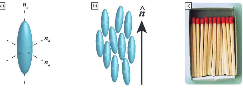
Figure 2.3: a) Example rod-like LC molecule and anisotropy in index of refraction. b) LC in the nematic phase. c) A macro-scale analog to LCs, matchsticks in a box exhibit partial order.
Anisotropy
Broadly speaking, anisotropy is a property of directional dependence. LC molecules are typically shaped like rods or discs, and this asymmetry causes the LC molecules to exhibit certain anisotropic properties. The most important anisotropy is in the index of refraction and is called the birefringence ∆n, defined as:
∆n=ne−no (2.7)
where ne is the extraordinary index of refraction and no is the ordinary index of refraction. In a uniaxial crystal, no is the index of refraction seen by light polarized in two of the crystal axes andneis the index of refraction seen by light polarized in the remaining axis, as shown in 2.3(a).
Dichroism is another anisotropic property of LCs, in which light polarized along different axes experiences different absorption. However, dichroism is generally negligible in LCs, and so our attention will be focused on their birefringence.
As both birefringence and dichroism are intrinsically related to polarization, it is only natural that LCs are useful for manipulation and detection and polarized light via elements such as GPHs.
Partial Order and The Nematic Phase
liquid phase is characterized by molecules that are not structured or ordered; molecules are free to move about or be reoriented as forces dictate. The solid phase is characterized by molecules that are very structured or ordered; molecules are spaced at regular intervals in a chemically bonded lattice and are not able to be moved or reoriented. Matter in a liquid crystal phase (a phase in-between the liquid and solid (crystal) phases) has molecules that are somewhat free to move and be reoriented, but are also somewhat structured and predictable. This later property is called partial order.
There are many liquid crystal phases that exhibit different degrees and different kinds of partial order. In this dissertation, we exclusively utilize the nematic phase. In the nematic phase, molecules do not posses any degree of positional order; i.e., the spacing between molecules is random and unpredictable. However, the molecules posses orientational order;i.e., the orienta-tion of the molecules is not entirely random and is somewhat predictable. In the nematic phase, the LC molecules will be oriented in an average direction, specified by a vector n called the nematic director. An example of LC in the nematic phase is shown in 2.3(b). A macro-scale analog of partial order and the nematic phase is matchsticks in a box, shown in 2.3(c). While the orientation of each individual matchstick is somewhat random, the matchsticks as a whole point in the same general direction. (We note that these matchsticks might be classified more accurately as being in a smectic phase rather than a nematic phase.)
The degree to which molecules are oriented to n is specified by a parameter S, called the order parameter. If the order parameter is 0, it indicates that the molecules are randomly oriented and are in the isotropic phase (equivalent to the liquid phase). A low non-zero order parameter indicates that the molecules are very loosely oriented ton; a higher order parameter indicates the molecules are strongly orientated to n. An order parameter of 1 will only occur if the molecules are perfectly ordered equivalently to a crystal lattice. The LCs used in this work have order parameters of ∼0.6.
Polymerization
In this work, we use a special class of LCs called liquid crystal polymers (LCPs). In contrast to typical liquid crystals such as those found in LCDs, the molecules in an LCP film are solidified and unable to move. Essentially, the nematic director is frozen in place, and the film becomes mechanically robust and relatively immune to external forces such as electric fields or mechanical pressure. This is highly advantages for films subject to a variety of atmospheric conditions or which do not need to be altered (static elements).
2.2.2 Alignment of Liquid Crystals
Understanding the alignment of liquid crystals,i.e., what the value ofnis, is of vital importance to creating functional LC elements. A vast amount of research has been done into understand-ing how material parameters, boundary conditions, applied electric or magnetic fields, dopant concentrations, and more affectn. We will focus here on methods developed to align LCs (i.e., setn) to desired in-plane angles. We define an in-plane orientation as ann that is parallel to a substrate and with some polar angle θ with respect to the substrate plane (i.e., ifz is normal to the substrate, n lies is in thex−y plane).
The physics of LC alignment can be easily understood from the vantage of minimization of energy states. Consider a handful of matchsticks like those in 2.3(c), which are shaped much like LCs. The matchsticks are put in a matchstick box without any care. Some of the matchsticks will fall into the box completely, some will be half in the box and half propped up by the walls of the box, and some will sit completely on top of the box. If you agitate the box by shaking it slightly, the matchsticks will all fall into the box completely (ignoring those that fall off the box completely) and all be aligned in the same general direction as dictated by the walls of the narrow box . This example demonstrates that the minimum energy state of the matchsticks is set by the boundary conditions imposed by the box, and when some amount of free energy is applied to the system (i.e., shaking) the matchsticks naturally go to the minimum energy state. So it is with LCs: as the molecules are not bound together, there exists some amount of free energy (e.g., thermal energy) enabling the molecules to move and reorient themselves [26]. The molecules will naturally “fall” into the minimum state as dictated by surrounding boundary conditions or by other external forces (e.g., an applied electric field [27]).
Surface Rubbing
One of the oldest and still most common methods of aligning LCs is by surface rubbing. In this method, a substrate is coating with a special alignment material designed to strongly influence the LC director. The substrate is then rubbed repeatedly with an abrasive material such as felt. The rubbing causes physical grooves or striations to form in the alignment material; essentially, aligning the alignment material. LC is then placed on the substrate and it aligns according to the alignment material (i.e., according to the rubbing direction). In the case of an LC cell such as in LCDs, two substrates are prepared, alignment material is aligned on each substrate individualy, the substrates are placed together to form a cell, and the cell is filled with LC.
Photoalignment Dopants
will align themselves to incident polarized light of specific wavelengths; if the dopant is already chemically attached the LC molecules, then aligning the dopant molecule directly aligns the LC molecules as well. If the dopants are not attached to the LC molecules, but are rather dis-persed in the LC, then the dopant molecules will indirectly align the LC molecules by imposing boundary conditions on the LC molecules and influencing the minimum energy states.
Photoalignment Films
Still another alignment technique is to use a photosensitive alignment material on the surface of a substrate [29, 30]. The alignment material is aligned by incident polarized light, then LC is placed on the alignment material and aligns accordingly. This is the method of alignment used throughout this dissertation.
Comparison of Alignment Methods
Both photoalignment dopants and photoalignment films allow for complex alignment patterns to be recorded which are otherwise impossible or practically infeasible with surface rubbing. Examples are the recording of polarization holograms such as the polarization grating [11] or the capture of entire holographic scenes [31]. Between these two photoalignment methods, using dopants is in principle more attractive. In practice, however, photoalignment films have better characteristics; namely, they enable LC films with higher birefringence and lower defects than LC films using photoalignment dopants. The work in this dissertation uses photoalignment films with linear photoalignment polymers (LPP), which are molecules sensitive only to linearly polarized light.
2.2.3 Fabrication of LC Films
Here we describe the basic steps used in this dissertation to fabricate LC films. Fabrication begins by coating a clean substrate with LPP, which coating is accomplished via spin coating. Spin coating is a thin-film coating technique in which a material is dropped onto a substrate and the substrate is spun at high speeds. The spinning causes most of the material to fly off of the surface, but intermolecular forces (i.e., surface tension and adhesion) cause a thin film to remain. By adjusting the acceleration and velocity of the spin, the thickness of the film can be controlled to within tens of nanometers in a highly repeatable fashion. Combined with simplicity of use and relatively low cost, spin coating is an extremely popular coating technique and is the coating technique used in this dissertation.
~1 mm ~0.1 µm ~2 µm
LC director
Figure 2.4: Cross section of LC films fabricated in this dissertation.
After LPP alignment, LCP is coated, again via spin coating. After being coated, the LCP is polymerized via a UV light source. At this point, additional layers may be added on top of the existing LCP film. For subsequent layers, the polymerized LCP serves as the alignment layer instead of the initial LPP. By adding more layers with specific spin parameters, any desired retardation may be achieved, typically half-wave retardation for some design wavelength. The final structure is shown in Fig. 2.4.
To summarize, LC films are fabricated as follows:
1. Coat LPP
2. Expose LPP
3. Coat LCP
4. Polymerize LCP
5. Repeat 3-4 as needed
2.3
Electromagnetic Waves
It is well known that light is an electromagnetic wave, composed of oscillating, orthogonal electric and magnetic fields. In this section, we review some key properties of electromagnetic waves which will be used throughout this dissertation.
2.3.1 The Electromagnetic Wave Equations
∇2E=µ∂2E
∂t2 (2.8a)
∇2B=µ∂
2B
∂t2 (2.8b)
where∇2 is the Laplacian,E is the electric field, andB is the magnetic flux. In this work, we
only consider materials with zero magnetic susceptibility, makingµ=µ0. Thus, we only need
consider the electric field, and the magnetic flux can later be derived via Ampere’s law:
∇ ×B=µ0
∂E
∂t. (2.9)
For most of this dissertation, we are concerned with waves which are monochromatic and have steady-state solutions. If the spatial extent of a wave is long compared to its wavelength, we can assume the wave has a steady-state solution. This is almost always the case. For example, a visible light source which is turned on for only 1 ns still has a spatial extent over one million times its wavelength. In addition, light sources which contain many wavelengths can in general be analyzed as a superposition of many monochromatic waves. For monochromatic waves of wavelengthλwith sinusoidal steady-state solutions, a general solution to the wave equation is:
E(r, t) =E(r) cos(ωt) =E(r) cos(kc0t) =E(r)Re{e−jkc0t} (2.10)
whereω is the angular frequency, k= 2π/λis the wavenumber,r=xˆx+yˆy+zˆz is a position vector, andc0 is the speed of light in a vacuum. Thus, the time dependent component is trivial
and only E(r) needs solved for.
2.3.2 Infinite Plane Wave Solution
A simple and highly instructive solution to the wave equation is an infinite plane wave. In complex exponential form, an infinite plane wave in a vacuum is:
E(r) =E0e−j(k·r+φ)pˆ (2.11)
where kis the wavevector, E0 is the wave amplitude, φ is an arbitrary phase constant, and ˆp
2.3.3 Diffraction
When a wave encounters an inhomogeneous medium, the solution to the wave equation quickly becomes very complex. If we consider a plane wave hitting an opaque sphere (i.e., the wave does not pass through the sphere), we can qualitatively describe the wave as bending or deforming around the sphere (in addition to reflecting back). While the initial plane wave propagated in a single direction, ˆk, the wave after the object is now traveling in many directions; indeed, the wave is now traveling in all possible directions to some extent. This phenomena, the redirection of light after encountering an obstacle, is called diffraction.
As the subject of diffraction is extremely broad, we will limit out discussion by introducing the following assumptions: 1) diffraction only occurs at the plane z = 0, 2) all space beyond z = 0 is a vacuum, and 3) the fields atz = 0 are known (this is nearly equivalent to knowing the structure before z = 0, i.e., the incident wave has passed through the structure but has not yet diffracted, and is a good approximation if the structure is thin). We also define the diffraction apertureDas the diameter of the physical structure; the structure may be an object in a vacuum or a void or structure in an otherwise homogeneous plane of material.
2.3.4 General Solution
A general solution to the diffraction problem may be obtained using Huygens’ principle. Huy-gens’ principle states that the propagation of any wave may be determined by decomposing a known wavefront into an infinite number of spherical wave sources. A solution to the diffraction problem stated above is thus:
E(x, y, z) = z jλ
Z ∞
−∞
Z ∞
−∞
E(x0, y0,0)e
−j2λzπr
r2 dx
0
dy0 (2.12)
wherer = ((x0−x)2+ (y0−y)2+z2)0.5. This equation is nearly always solved numerically.
Mathematical Approximations
A large number of mathematical approximations have been developed which can provide an-swers very close to the real solution. These various approximations are each based on different assumptions, and are thus only valid under certain conditions. In general, the most important parameter when choosing the appropriate mathematical model is the Fresnel number, defined as:
F = D
2
Lλ (2.13)
Near Field
When F >
∼1, the waves are in what is called the Near Field or Fresnel zone. This zone is the
most complex. The fields in this zone can be approximated using the Fresnel diffraction integral:
E(x, y, z) = e jkz
jλz Z ∞
−∞
Z ∞
−∞
E(x0, y0,0)e−j2λzπ[((x−x
0)2+(y−y0)2]
dx0dy0 (2.14)
This integral is still very hard to solve analytically, but is easier to solve numerically than the general solution.
Far Field
When F 1, the waves are in what is called the Far Field or Fraunhofer zone. This is the zone we will be working in for the majority of this work. In this zone, the relative field values do not change with z, but are scaled versions of each other, i.e., for any plane z1 and z2 in
the far-field, there is some ξ such that E(x, y, z1) = E(ξx, ξy, z2). A more convenient way to express this, is that the amount of power propagating in a given direction is constant. Thus, we usually speak of the Far Field in terms of wavevectors, not spatial coordinates. The Far Field can be approximated using what is called the Near-To-Far-Field Transformation (NTFFT):
E(kx, ky) = Z ∞
−∞
Z ∞
−∞
E(x0, y0,0)e−j(kxx0+kyy0)dx0dy0 (2.15)
wherekx = 2πα/λ,ky = 2πβ/λ, andαandβare the direction cosines defined by the wavevector:
k= 2π
λ(αˆx+βyˆ+γˆz). (2.16) Critically important is the fact that Eq. 2.15 has the form of a Fourier transform. Thus, this equation tells us that the near fields (fields directly after the structure) and far fields (fields infinitely far beyond the structure) are related via the Fourier transform; a fact that provides invaluable insight into the design and operation of diffractive elements.
2.4
Electromagnetic Finite-Difference Time-Domain Simulation
Time 1 Time 2 Time 3 Polarization Grating
Figure 2.5: Fields propagating through a PG; red and blue colors indicates positive and nega-tive fields respecnega-tively. This result was obtained using a version of the FDTD method developed in this work (see Chap. 7) and is extremely difficult if not impossible to obtain with analytic methods.
[34], rigorous coupled wave analysis [35], finite-element methods [36], and finite-difference time-domain (FDTD) methods [37]. In this work, we focus on the FDTD method.
The FDTD method is advantageous because it makes what are arguably the least number of assumptions about the electromagnetic fields or elements in question when compared to other simulation methods. Because of this, almost any arbitrary structure can be simulated and many phenomena may be observed, such as plasmon interactions, charge accumulation, evanescent waves, reflection, scattering, interference, and coherence. For example, with FDTD the fields propagating through a PG can be relatively easily obtained (Fig. 2.5). However, this diversity comes at a cost: FDTD simulations are generally very time-consuming, requiring vast amounts of computing power. For this reason, many specific FDTD algorithms are developed to simulate specific classes of elements at higher efficiency than with a generic FDTD algorithm.
2.4.1 Mathematical Basis
The FDTD method is based on approximating derivatives using linear algebraic expressions. The first-order central-difference approximation of a first and second order derivative are:
∂f(t) ∂t '
f(t+ ∆t/2)−f(t−∆t/2)
∆t (2.17a)
∂2f(t) ∂t2 '
f(t+ ∆t)−2f(t) +f(t−∆t)
∆t2 (2.17b)
where ∆tis the time step. It can be shown that the error of the approximation is related to the size of the time step, with smaller time steps resulting in less error.
Figure 2.6: The grid scheme used in this work is the 3D Yee grid; shown is a unit cell with the location of theE and Hfields).
∂
∂t 0rE
+σE=∇ ×H (2.18a)
∂
∂t µ0µrH
=−∇ ×E. (2.18b)
The FDTD algorithm works by substituting the finite-difference approximations for the time derivatives, and solving for future time steps E(t+ ∆t) andH(t+ ∆t) based on current time stepsE(t) andH(t). The curl operator is also approximated, using spatial equations analogous to 2.17b. Thus, the fields are solved for on a discrete grid of points spaced ∆u apart.
2.4.2 The Yee Cell
E=ˆxEx((i+ 1/2)∆u, j∆u, k∆u)+ ˆ
yEy(i∆u,(j+ 1/2)∆u, k∆u)+ ˆ
zEz(i∆u, j∆u,(k+ 1/2)∆u) (2.19a)
H=ˆxHx(i∆u,(j+ 1/2)∆u,(k+ 1/2)∆u)+ ˆ
yHy((i+ 1/2)∆u, j∆u,(k+ 1/2)∆u)+ ˆ
zHz((i+ 1/2)∆u,(j+ 1/2)∆u, k∆u) (2.19b)
where i,j, andk are integers. When applying the finite-difference approximations as previous described using this grid scheme, the E and H fields are solved for one after the other in subsequent time-steps using a leap-frog technique; E(∆t+ 1) is solved for using E(∆t) and
H(∆t+ 1/2), then H(∆t+ 3/2) is solved for using H(∆t+ 1/2) and E(∆t+ 1). The details of how this algorithm works may be found in a multitude of literature [38].
2.4.3 FDTD Summary
Chapter 3
Direct Write System for CGH
Creation
This chapter takes the form of a manuscript accepted to Optics Express, whose authors are Matthew Miskiewicz and Michael Escuti.
Abstract
We1 report on a direct-write system for patterning of arbitrary, high-quality, continuous liquid crystal (LC) alignment patterns. The system uses a focused UV laser and XY scanning stages to expose a photo-alignment layer, which then aligns a subsequent LC layer. The exposure of the alignment layer utilizes overlapping exposures, which sometimes results in interesting responses by the LC and ultimately enables us to create continuous alignment patterns with feature sizes less than the beam size. We present our system design and a thorough mathematical system description, starting from the direct-write system inputs and ending with the alignment of the LC. We fabricate a number of patterns to test the accuracy of our predictions, then design and fabricate a number of interesting patterns including aq-plate and polarization grating.
3.1
Introduction
Liquid crystals (LCs) are most prominently used in liquid crystals displays (LCDs), where they function as the active elements used to control pixel brightness. In these cases, the alignment of the LC is simple, being homogeneous over relatively large areas. However a number of other
1
applications require complex LC alignment patterns for correct operation. Examples of such elements are polarization gratings (PGs) [1], q-plates [39], beam shaping elements [18], phase plates [3], and LC actuators [40].
With the rise of photo alignment materials [30, 41], the alignment patterns required for such elements has become easier to realize using polarization holography [42]. However, while polarization holography is quite suitable for periodic patterns such as the PG, it does not solve the problem of easily aligning more arbitrary patterns.
In recent years, various photo-alignment techniques have been developed to efficiently record specific patterns. These include scanning a cylindrical beam while changing the polarization to record a PG [43], scanning a cylindrical beam in an azimuthal pattern while changing the polarization to record a q-plate [39, 44], using a reconfigurable spatial light modulator (SLM) to record arbitrary patterns including a lens array [45], and using a point-by-point direct-write system with a polarization modulator to record a complex beam-shaping element [18]. It is notable that this last kind of direct-write system is actually quite old, as the first reported direct-write system with polarization modulation dates back to 1976 [16].
In this paper, we present, analyze, and demonstrate a direct-write system capable of creating arbitrary and continuous LC patterns (in-plane orientation profiles) with high quality and resolution. The system design and operation is discussed in Section 2. In Section 3, we develop a flexible system description starting with the direct-write scan inputs and ending with the LC response. Although we use the system with photoalignment materials and LCs, the system description is applicable to any material set sensitive to linear polarization. In Section 4, we fabricate a few patterns to test the accuracy of our system description and its ability to predict the LC response. In Section 5, we use the parameters obtained from Section 4 to study some interesting patterns, including adjacent scan lines to explore the continuous nature of the LC alignment, intersecting scan lines to study non-intuitive LC responses, and a highest quality q-plate and PG.
All of our results indicate that this approach is by far the most flexible and diverse LC patterning approach, allowing the creation of arbitrary continuous LC patterns. In addition, the approach can be easily scaled for large areas and volume manufacturing, where multiple high resolution LC patterns can be created on the same substrate.
3.2
System Design
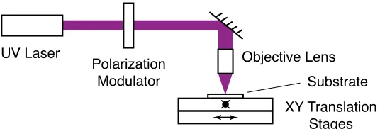
polariza-UV Laser
Polarization Modulator
Objective Lens
XY Translation Stages Substrate
Figure 3.1: High-level schematic of the kind of polarization direct-write system studied in this paper.
tion modulators include a rotating HWP or a variable retarder combined with a quarter wave plate (QWP) (when configured properly, these two elements rotate the polarization angle as the retardation is changed). Our system uses the later, with a KD*P Pockels cell by ConOptics as the variable retarder. After this, the laser passes through a spatial filter and a collimating lens (not shown in figure). Last, the beam is focused to the substrate with a 40X objective lens. The minimum beam waist [46] we have achieved with this setup is∼1 µm.
The substrate itself is coated with a linear photopolymerizable polymer (LPP) and is placed on two stages for XY translation. The stages are from Newport (ILS200LM) and have 10 nm resolution. Since even the smallest beam waist is 100 times this resolution, the resolution and accuracy of the XY stages is neglected in the analysis. The entire system is controlled via a Newport XPS controller.
After exposure, the substrate is removed and a liquid crystal polymer (LCP) layer is spin cast on top of the LPP layer, then polymerized by UV light. If needed, multiple layers of LCP can coated. Alternatively, two LPP coated substrates forming a cell can be used in place of a single LPP coated substrate. In this case, a non-polymerizing LC may be used to fill the cell, allowing the pattern to be toggled on or off with an applied voltage. However, we restrict the current discussion to LCP coated on a single substrate with LPP, although we expect the principles should apply to cells as well.