ABSTRACT
BEAM, ANDREW LANE. A Bayesian Framework for the Analysis of the Peroxisome Proliferator-Activated Receptor Signaling Pathway. (Under the direction of Alison Motsinger-Reif.)
Toxicology is currently developing computational tools to assess chemical hazard and risk using high-throughput screening assays. These approaches often employ pathway-based or “Mode-of-Action” analyses to understand how a compound may affect an organism. One such set of pathways are those triggered by the interactions of chemicals with the
A Bayesian Framework for the Analysis of the Peroxisome Proliferator-Activated Receptor Signaling Pathway
by
Andrew Lane Beam
A thesis submitted to the Graduate Faculty of North Carolina State University
in partial fulfillment of the requirements for the degree of
Master of Science
Statistics
Raleigh, North Carolina 2011
APPROVED BY:
_______________________________ ______________________________
Dr. Alison Motsinger-Reif Dr. Richard Judson
Committee Chair
________________________________ _______________________________
DEDICATION
For Nana:
BIOGRAPHY
ACKNOWLEDGMENTS
TABLE OF CONTENTS
List of Tables ... vi
List of Figures ... vii
List of Equations ... viii
Chapter 1 Introduction...1
1.1 Background and Motivation ...1
1.2 Peroxisome Proliferator-Activated Receptor (PPAR) ...3
1.3 Hierarchical Bayes Models and MCMC Methods ...9
Chapter 2 Methods ...14
2.1 Data Description ...14
2.2 Graphical Model Description ...17
Chapter 3 Results ...20
3.1 Variable Selection and Preliminary Analysis ...20
3.2 Contribution of Each Variable to the Model and Convergence Assessment ...24
3.3 Discussion and Future Directions ...36
References ...38
Appendices ...41
A.1 R Code ...42
LIST OF TABLES
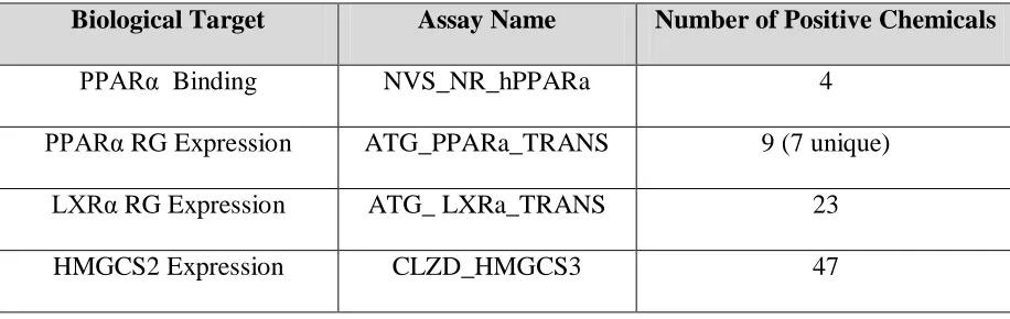
Table 1: Summary of assays used in final model ... 21 Table 2: Parameter estimates for simple model ... 26 Table 3: Parameter estimates from model including PPARa binding and LXRα-driven
suppression of PPARα RG expression ... 29 Table 4: Parameter estimates from model including PPARa binding and LXRα-driven
LIST OF FIGURES
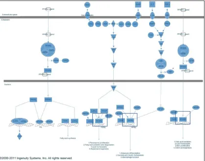
Figure 1: Pathway Map for PPAR Signaling (KEGG) shows the signal cascade leading to PPAR activation. The three isoforms, PPAR-α/δ/γ, are boxed in blue... 5 Figure 2: An alternate pathway map for PPAR signaling from Ingenuity Systems, Inc. PPAR-α/δ/γ are boxed in blue. ... 6 Figure 3: Measurement error model of the PPARα neighborhood represented as a graph. The dark ovals represent the true, unobserved biological values and the light blue nodes represent the response values observed in the assays. The grey epsilon nodes represent random error associated with each observation. ... 17 Figure 4: Scatter plots investigating the relationships between parent-child nodes. ... 22 Figure 5: Plot showing PPARa RG vs. LXRa RG responses. This plot is suggestive of a negative, nonlinear relationship between the parent node LXRα RG and the child node
LIST OF EQUATIONS
Equation 1 ... 10
Equation 2 ... 10
Equation 3 ... 10
Equation 4 ... 13
Equation 5 ... 13
CHAPTER 1
Introduction
1.1 Background and Motivation
Toxicology is the science concerned with the study of chemically induced adverse effects on biological systems and living organisms. An adverse effect may refer to maladies ranging from mild discomfort, specific system failure, all the way to chemically triggered death (1). Chemical toxicity, risk, and hazard have traditionally been assessed using observational animal studies (2). Typically these studies divide a cohort of animals into different dosage levels of the chemical under study and the effects (i.e. tissue lesions, tumor formation, or subject death) are recorded after a fixed amount of time. Next, standard statistical tests are performed to see at what level the treatment chemical differs from the control group and this is taken as an estimate as the lowest effect level (LEL). These studies typically take years and cost millions of dollars to complete (3). Furthermore, these types of studies often lack a mechanistic explanation of the chemical’s mode of toxicity, making comparisons with future chemicals difficult. Recently there has been a growing effort to move toxicity from an observational science to a predictive one. Recent advances in high-throughput assay technology have made it possible to produce large volumes of data at the granularity needed for such an endeavor. Moreover, these types of mechanistically targeted data are being use to perform pathway-based or “Mode-of-Action” analyses, where the data are used to infer the mode or mechanism a compound is taking to cause the adverse outcome.
model described will leverage the structure and relationships in these data that have been mined from the biological and toxicological literature to create a more biologically informed and relevant model. We will show that the use of these methods result in a set of analytical tools that is more reflective of how a chemical may affect a living organism. In particular, the data we start with is derived from in vitro (cell-based or cell-free) assays that probe different nodes of the pathway. These assays are noisy (i.e. they produce some number of false positive and false negative calls). The overall goal here is to integrate noisy data across many chemicals and many nodes of the pathway to produce posterior statements about whether each chemical does or does not interact with the pathway.
1.2 Peroxisome Proliferator-Activated Receptor (PPAR)
Peroxisome proliferator-activated receptors (PPARs) represent a set of nuclear receptor proteins that function as ligand-dependent transcription factors that are involved in gene expression. Three isoforms have been discovered and named as PPAR-α/γ/δ according to differential tissue distributions and biological profiles (4). PPARα is primarily expressed in liver, heart, muscle, and kidney tissue and is involved with lipid and fatty acid metabolism (5).
Compounds that activate PPARs are known as peroxisome proliferators (PPs). It has been shown PPAR activation can be achieved by compounds with a broad spectrum of structures and functions. Several adverse effects have been associated with PPs including diabetes, obesity, atherosclerosis, and hepatocellular carcinomas. It has been proposed that PPARα is profoundly involved in mediation of these events; however the species difference between rodents and humans in PPARα is not yet fully understood (4).
Both representations of the pathway give similar topologies and connections for PPAR signaling, with a few minor exceptions that will be discussed later. From these maps we will introduce the notions of “upstream” and “downstream” relative to PPAR. In this treatment, we will focus on the PPARα pathway, but similar analyses could be performed for the other isoforms. An element in the pathway is said to be “upstream” of PPARα if it occurs
before chemical interactions with PPARα takes place. Similarly, an element is “downstream” of PPARα if occurs after chemical interactions with PPARα. If we view PPAR signaling as a directed graph, then the notions of upstream and downstream correspond to parental and children nodes respectively, relative to the node representing PPARα expression. We will adopt this graph theoretic notation more fully in later sections. Note that there is also a causal
interpretation of these signaling pathways. Each element along the pathway is caused by the elements preceding it. PPARα activity (as measured by assays that detect PPAR-mediated expression of mRNA or proteins) is caused by the elements upstream of it in the pathway, and in turn, PPARα activity contributes to causal influences of the elements further downstream.
When assessing a compound’s effect on PPARα, typically in vitro or in vivo
(PPRE). A secondary path is through Mitogen-activated protein kinase 3 (MAPK3 is a synonym for ERK1/2 shown in Figure 2), where activation of MAPK3 leads to elevated expression levels for PPARα, which then again heterodimerizes with RXRα and continues further to regulate gene expression.
Several issues arise when trying to measure PPARα activity both in vivo and in vitro.
In vivo levels must be measured in a surrogate species, as it requires the subject to be sacrificed to assess, and this is most often done in rodents. However, these studies are both slow and expensive, making screening any more than a few chemicals simultaneously intractable. Furthermore, there is a species difference for PPARα between rodents and humans, making interpretation of results difficult and unclear. Despite most of these issues, an in vivo study is currently used as the gold standard for assessing a compound’s PPARα activity.
Another source of assay interference is that as the concentration of a chemical approaches the level at which cells die (cytotoxicity), cells often turn pathways on or off in a chemical-independent way, again confounding our ability to understand chemical-specific effects. However, these types of issues tend to be assay or technology-specific, so by combining data from multiple assays and technologies for the same pathway, one can in principle control for these false-positive and false-negative findings in specific assays.
1.3 Hierarchical Bayes Models and MCMC Methods
Bayesian methods for inference are a set of approaches for drawing conclusions from data conditioned on a probability model. The hallmark of Bayesian inference is the explicit role that the probability model serves in quantifying uncertainty during the analysis process and for summarizing the results through a probability distribution on the parameters under study (9). First, we introduce some notation and the basic concept of a probability density. Let x be the observed data vector and θ be the unobserved population parameters of interest.
Typically it is the goal of an experiment to estimate θ. Next, p(x|θ) represents the conditional
probability density function for values of x given a fixed value for θ and p(x) represents the marginal probability density function of x. This allows us to calculate the probability of a given event, such as p(x > 0) = . However, we may use this notation for inference about the population parameters through the use of the likelihood function. In the likelihood, L(θ|x), the data are viewed as fixed and used to estimate the population
probability density function have the same form for a given family of probability distributions, the only difference being how one views them. From the likelihood
perspective, we view our data sample as being fixed and use it to estimate the population parameters, whereas the density function views the parameters as fixed and the aim is to make statements about future observations.
The namesake of Bayesian inference procedures comes from the repeated use of Bayes’ rule. Again, letting x represent our data vector and θ be the parameter vector, Bayes’ rule is stated as follows:
Equation 1
This relationship factors the joint probability distribution of x and θ in terms of the marginal distribution of θ and the distribution of x conditioned on θ. A common and equivalent method of writing Bayes’ rule is:
Equation 2
which yields the normalized posterior likelihood for θconditioned on the data sample of x. In Bayesian terminology, p(θ) is the prior distribution for θ, encapsulating knowledge or
uncertainty about the unknown parameters. Again, we are typically interested in inference about the population parameters θ, given our set of observations. With this in mind we can rewrite the Bayes’ rule as:
This yields an unnormalized ( indicates “proportional to”) posterior distribution for θ given
our set of observations x. Given a fully specified probability model for both x and θ, Bayes’ rule allows for inference about the quantity θ, given the observed values of x. This forms the core of Bayesian inference procedures.
Hierarchical Bayes models are a set of approaches used to encapsulate and model randomness that occur at multiple levels. The fundamental concept is the notion of
hyperparameters. Hyperparameters are elements from the prior distribution which are themselves random. For example, the prior distribution for the variance of a normal random variable may follow a gamma distribution whose shape and scale parameters themselves follow some other probability distribution. All Bayesian models may be viewed as inherently hierarchical because the prior distribution on θ represents the first level and the
likelihood/posterior p(θ |x)represents the final level of the hierarchy (7). These models are easily represent as directed, acyclic graphs with the top-most hyperparameters being the top parental nodes and the bottom-most child nodes being the final posterior distributions. Each node in this graph encapsulates quantitative probability information about a variable of interest (8). In the computer science literature, these types of models are often referred to as
For complex probability models, the posterior distribution may not be able to be expressed in closed form. For situations such as these, Markov Chain Monte-Carlo (MCMC) methods are typically used to evaluate and analyze the posterior (9). These approaches represent a class of samplers for generating data from the posterior used for the inference. Once such technique is the Gibbs sampler, which is implemented in the well known WinBUGS software platform (10). MCMC methods can be used to generate samples from the true posterior distribution and inference is made using these samples. This is done by constructing a Markov chain whose stationary distribution is the desired posterior distribution. Constructing this chain is usually straight forward; however for subsequent inference to be correct, checks must be carried out to insure that the chain has converged to its stationary distribution. A common graphical check is done by running multiple
simultaneous chains and plotting their values over the final period for the simulation and qualitatively inspecting if the chains are well mixed. A more quantitative approach offered by Gelman and Brooks is the potential scale reduction, , (11) which monitors the factor by which the current distribution might be reduced as the number of iterations grows. For close to 1 (often values less than 1.1 are sufficiently close to 1 (9)), the Markov chain is thought have converged to the desired posterior distribution.
Equation 4
where C is a constant that gets canceled during the comparison process and is irrelevant. The expectation of the deviance with respect to θ is typically denoted as . Next, we define the effective number of parameters in the model as:
Equation 5
where is the deviance for the expected value of θ. Finally, the DIC is computed as:
Equation 6
Models with smaller DIC are to be preferred to models with larger DIC. Thus DIC, like AIC and BIC, attempts to strike a balance between the number of parameters in the model (pD)
and how well the model fits the data ( ). DIC is often used in Bayesian approaches because it can be easily calculated from MCMC simulations, whereas AIC and BIC require
CHAPTER 2
Methods
2.1 Data Description
The U.S. Environmental Protection Agency’s ToxCast ( (12), (3) ) is measuring in vitro activity in a battery of over 500 high-throughput assays in a collection of ~1,000 environmental and industrial chemicals, and using this data to construct pathway-based models of toxicity. The National Research Council has advocated for this type of molecular-based in vitro toxicity testing as a practical way to manage the lack of toxicity information for the vast majority of environmental chemicals (2). In this study we will focus on data for 309 environmental chemicals in a subset of assays probing targets in the PPAR pathways. For a more comprehensive treatment of this data set, see (13).
The data used to build and evaluate the model represent four distinct technologies from Attagene Inc. (12), the CellzDirect/Life Techonologies Corporation (13), the NIH Chemical Genomics Center (“NCGC”, (14)), and Novascreen, Inc (15). Datasets from these technologies measure various points in the PPARα pathway. A cell-free competitive binding assay (assay key: NVS_NR_hPPARa) measures the binding affinity of a compound for the PPARα protein. The cell-free MAPK3 assay (assay key: NVS_ENZ_hMAPK3) is a
recombinant kinase assay that measures enzymatic activity. Two assays (assay keys: ATG_PPARa_TRANS, NCGC_PPARa_Agonist) measure expression of downstream reporter gene (RG) mRNA that is induced by the PPAR transcription factor which is
expression of hydroxymethylglutaryl-CoA synthase, mitochondrial (HMGCS2, assay key: CLZD_HMGCS2), which is a specific gene whose expression is regulated by PPAR.
Each observation used from the data is a measure of the amount of the respective biological target produced for each chemical-concentration-assay pair, hereto referred as the “response”. Each raw response is in units of the assay’s measurement method (typically fluorescence or luminescence) and was normalized by dividing the raw response of the compound by the measured value of negative control dimethyl sulfoxide (DMSO) to yield a fold-over-control (FOC) value. All assays were run in concentration-response format, and the response was fit to a 4-parameter logistic model to derive a characteristic activating
concentration, which is the AC50 (concentration at which 50% of maximal activity is seen). Compound-assay combinations were also characterized by whether there was any activity seen over the concentration range tested (hit vs. no hit). For the ATG_PPARa_TRANS assay, 7 chemicals were identified as hits: Bromoxynil, Diclofop-methyl, Diethylhexyl phthalate (DEHP), Fenthion, Imazalil, Lactofen and Perfluorooctanoic acid (PFOA). The chemicals identified as positive in this assay will be of interest to us because the assay is designed to be an indication of PPARα expression through the use of a reporter gene (RG) which is
regulated by PPARα. We will evaluate the model’s performance by examining how the model’s results deviate from this assay. Additionally, since there are two assays that attempt to measure PPARα expression levels through the use of a reporter gene
(ATG_PPARa_TRANS, NCGC_PPARa_Agonist), but use different technologies to do so, we will use one (ATG_PPARa_TRANS) to build the model and withhold the other
Since the data are derived from 4 separate technologies they were run on different sets of concentrations, all responses were interpolated to a common, synthetic set of
concentrations of {0.01,0.1,1,10,20,50,75,100} micromolar. If a compound was identified by the initial data analysis as active, the response was interpolated using the 4-parameter logistic model. If it was not identified as active, a simple linear regression was performed to
interpolate to the synthetic set of concentrations. If a compound did not have a full
2.2 Graphical Model Description
We wish to combine the datasets described in section 2.1 in a way that is reflective of the biological structure shown in Figures 1 and 2. The measurement error model for the PPAR-α neighbor is represented using a directed, acyclic graph (DAG) abstraction and assumes an additive measurement error term for each observation. This is shown below:
Figure 3: Measurement error model of the PPARα neighborhood represented as a graph. The dark ovals represent the true, unobserved biological values and the light blue nodes represent the response values observed in the assays. The grey epsilon nodes represent random error associated with each observation.
may act via directly binding to the PPARα protein, represented by the “PPARα Binding” node in graph. It may also act by binding to mitogen-activated protein kinase 3 (MAPK3). The effect of this is to enhance the effect of PPARa transcription. The activity at the PPARα RG node is a result of both ligand binding and MAPK3 activity, though this exact
relationship will be specified later. Similarly, we see that biological endpoints further downstream, such as HMGCS2 are influenced by PPARα activity.
Thus far we have specified the causal relationships reported in the biological literature, but have not specified a mean model for the parent-child relationships. One approach is to assume that each child’s expected value is a linear combination of its parents. Under this assumption the expected value of the PPARα RG node, conditioned on the values of its parental nodes would be:
because the parental nodes for PPARα RG in our measurement error model are the nodes for PPARa binding and MAPK3 activity. This model is attractive because it is easy to fit, simple, and has high interpretability. However, it has been shown that often relationships in genetic and biological networks cannot be accurately captured by linear models (12). Basis-splines, or B-splines, have been shown to be an attractive approach for estimating these potential nonlinear relationships automatically (13).
the expected value for the PPARα RG node is:
Finally, a well known model that incorporates the notations of exponential activation or suppression with asymptotic saturation is the 4 parameter logistic model (14). This model is defined by an upper and lower asymptote, an inflection point, and a factor known as the “hill-slope”, which is the rate at which the response grows or decays. The form of this model is:
where T and L are the upper and lower asymptotes respectively, C is the inflection point, and W is the Hill-slope. Typically the four parameters in these models are estimated under the least-squares criterion using nonlinear methods such as Gauss-Newton (15) or by using alternative methods (16). Returning to mean model PPARα RG, the expected value under this model is:
CHAPTER 3
Results
3.1 Variable Selection and Preliminary Analysis
To maximize the signal-to-noise ratio in the data used to build the model, we employed some simple heuristics to eliminate uninformative data. First, we performed a preliminary analysis of all endpoints shown in Figure 3, the graphical representation of the measurement error model. These assays represent measurements for direct nuclear receptor ligand binding (NVS_NR_hPPARa), MAPK3 enzymatic activity (NVS_ENZ_hMAPK3), PPARα RG expression (ATG_TRANS_PPARa), LXRα RG expression
(ATG_TRANS_LXRa), and HMCS2 expression (CLZD_HMGCS2). We eliminated assays that had three or fewer chemicals identified as positives in the EPA’s initial analysis. This eliminated the assays for RXRα RG (0 positives) and MAPK3 activity (3 positives). Recall that MAPK3 is from the Novascreen suite of assays, which was subject to an initial prescreen before any data analysis was performed. As a result, only 22 chemicals passed the initial prescreen and only 3 of these were identified later as positives. Thus there is no
concentration-response data for 298 chemicals, which makes the information content available from this assay quite low. The Novascreen assay for PPARa binding only had 4 chemicals identified as positives during the data analysis, but 118 chemicals passed the initial prescreen, meaning there was at least some data for a large portion of the chemicals.
across 4 assays that satisfied these initial selection criteria. The results are summarized below in Table 1.
Table 1: Summary of assays used in final model
Biological Target Assay Name Number of Positive Chemicals
PPARα Binding NVS_NR_hPPARa 4
PPARα RG Expression ATG_PPARa_TRANS 9 (7 unique)
LXRα RG Expression ATG_ LXRa_TRANS 23
HMGCS2 Expression CLZD_HMGCS3 47
Within the ToxCast chemical library, several chemicals were run in duplicate and triplicate to assess assay variance and to compute concordance measures. One of the compounds run in triplicate, Diclofop-methyl, was positive in the ATG_PPARa_TRANS assay for all three replicates. As such, all three replicates were included in the model building and evaluation process.
Figure 4: Scatter plots investigating the relationships between parent-child nodes.
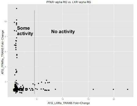
and convergence and DIC were poor for all three models discussed in Section 2.1. The final relationship decided upon for LXRα RG-PPARα RG for further analysis aims to capture the suppression relationship of LXRα RG on PPARα RG found in the literature. If we examine the plot of PPARα RG vs. LXRα RG more closely a potential model becomes evident. This is shown in Figure 5 below.
Figure 5: Plot showing PPARa RG vs. LXRa RG responses. This plot is suggestive of a negative, nonlinear relationship between the parent node LXRα RG and the child node PPARα RG.
place. From this, we propose the following functional relationship between PPARα and LXRα:
where z represents PPARα activity from other sources. In this formulation, LXRα acts on PPARα in manner similar to a step function, and for suitably large values, stops PPARα expression almost entirely. However, there is a discrepancy between the KEGG and Ingenuity pathway maps for the direction for this dependency. KEGG shows LXRα downstream from PPARα while the Ingenuity pathway map shows the reverse. However, KEGG pathway map shows PPARα leading to LXRα activity, which we do not see in the data (e.g. Figure 5). In truth, there may be a feedback mechanism between LXRα and PPARα, whereby PPARα RG expression leads to LXRα expression, which in turn limits the activity of PPARα. This type of mechanism cannot be modeled in a hierarchical fashion, as all dependencies must be acyclic. Considering this, we will use the place LXRα RG above PPARα RG in the hierarchy and assume its behavior as limiting PPARα RG.
3.2 Contribution of Each Variable to the Model and Convergence Assessment
First we model the simple process of PPARa binding leading to PPARα RG expression. The hierarchal model for this scenario is given as:
Next, we assume the observations from the dataset are jointly normal:
where I2 is the 2x2 identity matrix. Each X1j represents a data point for a given chemical at a
given concentration from the PPARa binding while each X2j represents a data point for a
given chemical at a given concentration from the Attagene PPARα RG data
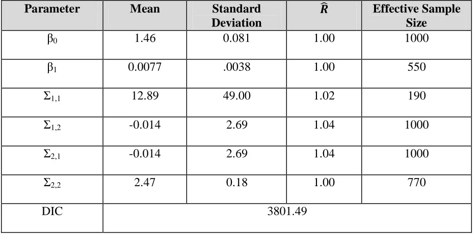
Table 2: Parameter estimates for simple model
Parameter Mean Standard
Deviation
Effective Sample Size
β0 1.46 0.081 1.00 1000
β1 0.0077 .0038 1.00 550
Σ1,1 12.89 49.00 1.02 190
Σ1,2 -0.014 2.69 1.04 1000
Σ2,1 -0.014 2.69 1.04 1000
Σ2,2 2.47 0.18 1.00 770
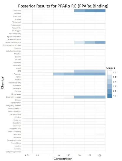
Figure 6 is a heatmap showing the posterior probability that PPARα RG expression will be greater than two times the control level. Each cell represents one chemical at one concentration. Two-fold over control was chosen for display purposes, as this level was anecdotally observed to be the noise-band in the PPARα RG expression data. This threshold was not used in the model in any way, but only used to determine the color intensity of each cell: darker colors correspond to higher posterior probabilities. The probability was
calculated by the dividing the number of posterior samples greater than two FOC by the total number of samples for the mean of a given chemical/concentration pair.
In this model, the only way to induce PPARα RG expression is by directly binding PPARa. Even though the diagnostic statistics for the model parameters are quite good, there is very little literature support for the chemicals identified as positive in the posterior, except for Perfluorooctanoic acid (PFOA). From this we conclude that this simplistic model is not sufficient to fully capture PPARα expression.
Next, we add LXRα RG to the model. The conditional dependency model is specified below.
An important point to note is that this model explicitly allows for PPARα RG activity even in absence of PPARa binding. We know that we do not have all possible sources for PPARα RG activity in our dataset, as we eliminated the assay for MAPK3 due to a lack of
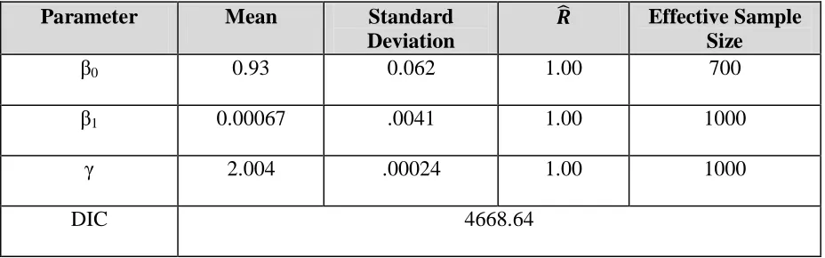
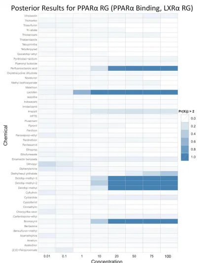
information content. However, the term attempts to mediate this lack of data by “trusting” the PPARα RG expression data so long as LXRα RG expression is not too high. The parameter estimates are shown in Table 3 (covariance parameters omitted, but all were found to have converged) and the posterior results are shown in Figure 7.
Table 3: Parameter estimates from model including PPARa binding and LXRα-driven suppression of PPARα RG expression
Parameter Mean Standard
Deviation
Effective Sample Size
β0 0.93 0.062 1.00 700
β1 0.00067 .0041 1.00 1000
γ 2.004 .00024 1.00 1000
The results for this model are encouraging, as many compounds identified in the literature as positive show a strong signal in the posterior. There is strong evidence in the literature that diclofop-methyl (4), lactofen (17), perfluorooctanioc acid (PFOA) (18) are potent in vivo
PPARα agonists and are capable of inducing PPARα activity in vitro. The only chemical with a strongly positive signal in the posterior not currently well supported in the literature is bromoxynil. However, as of May 2011 a literature search did not yield any evidence that bromoxynil is not a PPARα agonist, so it may be that this compound’s PPAR profile has not yet been well studied. Indeed our model suggests that it may be a PPARα agonist as it has PPARa Binding activity (~ 26 FOC at highest concentration), good PPARα RG expression (~ 5.6 FOC at highest concentration), and it does not induce LXRα (max of 1.1 FOC). All four chemicals that showed strong signals in the posterior also induced PPARα RG activity in the independent NCGC PPARα RG assay, which was not used in the model.
Three compounds that were identified in the initial analysis as positive for ATG_PPARa_TRANS have little to no signal in the posterior. These compounds are
fenthion, imazalil, and diethylhexyl phthalate (DEHP). Fenthion has been shown to not be a PPARα agonist in vitro (4) and there is no evidence which shows it to be an agonist in vivo.
consideration and was left out of the data used to build the model. At first glance this may be worrisome, but the relationship between DEHP’s and MEHP’s interaction with PPARα is complex and not yet settled. Also, it has been suggested that one of endpoints of concern with DEHP (liver tumors) may be caused by a pathway independent of PPARα (20). We will discuss the DEHP/MEHP-PPARα interaction further in the discussion section. Finally, fenthion, imazalil, and DEHP were negative in the NCGC PPARα RG assay as well, giving further corroboration to this model’s results.
Finally we evaluate the full model that includes HMGCS2. The conditional dependency model is specified below:
Finally, we again assume the observations are multivariate normal of the form:
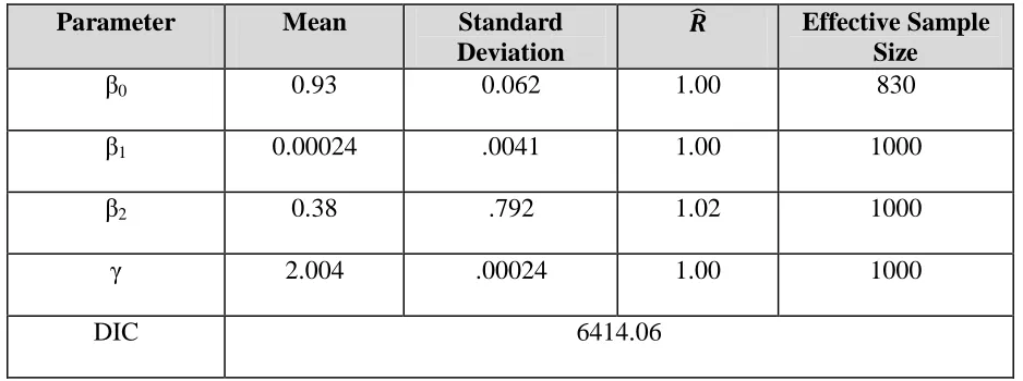
Table 4: Parameter estimates from model including PPARa binding, LXRα RG, and HMGCS2
Parameter Mean Standard
Deviation
Effective Sample Size
β0 0.93 0.062 1.00 830
β1 0.00024 .0041 1.00 1000
β2 0.38 .792 1.02 1000
γ 2.004 .00024 1.00 1000
3.3 Discussion and Future Directions
In this paper we have outlined a technique for combining multiple sources of
information about chemical’s potential activity in a biological pathway. We have shown how these biological pathways can be abstracted as graphs and then viewed in terms of
hierarchical models and Bayesian networks.
The results of this approach are promising. The raw data showed 9 chemicals (7 unique) as being positive for PPARα binding. However, when other sources of data related the PPARα signaling were incorporated, the posterior showed that only 4 unique chemicals had truly strong biological signals. Of these 4 positives, 3 had literature evidence
corroborating both in vitro and in vivo PPARα activity. We could not find any literature supporting Bromoxynil as a PPARα agonist, but we were also unable to find any literature to dispute this claim. Of the three compounds initially identified as positive for PPARa RG in the raw data but were not in the posterior, 2 (imazalil and fenthion) were supported by the literature as being negatives. While DEHP is largely thought to be a PPARα agonist, it is believed to activate this pathway through its metabolites, primarily MEHP. Since these assays have limited metabolic competency, it is not surprising that the DEHP’s posterior shows a weak signal according to conventional wisdom about the DEHP-PPARα
relationship. However, there is some dissent in the literature about the nature of DEHP’s, and consequently MEHP’s, agonist behavior on PPARα. The conventional notion that
believe that the apparent partial agonism we see in the posterior may be an accurate portrayal of complex and perhaps not yet fully understood interaction between DEHP and PPARα.
Finally, all 3 of these compounds were also negative in the separate and independent NCGC PPARα RG assay, strengthening the belief that the model is correctly identifying compounds that directly interact with PPARα. However, since the NCGC assay also has limited metabolic capacity, it too would miss compounds that interact with PPARα via a metabolite.
REFERENCES
1. Aldridge, W. N. What is Toxicology: a discussion of scientific developments in relation to practical need. 1985.
2. National Research Council. Toxicity Testing in the 21st Century: A Vision and a Strategy. Washington, DC : National Academies Press, 2007.
3. The Toxicity Data Landscape for Environmental Chemicals. Judson, Richard, et al. 2008, Environmental Health Perspectives.
4. In vitro screening of 200 pesticides for agonistic activity via mouse peroxisome
proliferator-activated receptor (PPAR)-alpha and PPAR-gamma and quantitative analysis of in vivo induction pathway. Takeuchi, Shinji, et al. 2006, Toxicology and Applied
Pharmacology, pp. 235-244.
5. Central Role of peroxisome proliferator-activated receptors in the actions of peroxisomes proliferators. Corton, J.C., Anderson, S.P. and Stauber, A. 2000, Annu Rev Pharmacol Toxicol, pp. 491-518.
6. KEGG: Kyoto Encyclopedia of Genes and Genomes. Kanehisa, Minoru and Goto, Susumu. 2000, Nucleic Acids Research, pp. 27-30.
7. Ntzoufras, Ioannis. Bayesian Modeling Using WinBUGS. Hoboken, New Jersey : John Wiley & Sons, Inc., 2009.
8. Russell, Stuart and Norvig, Peter. Artificial Intelligence: A Modern Approach. 2nd. Upper Saddle River : Prentice Hall, 2003.
9. Gelman, Andrew, et al. Bayesian Data Analysis. s.l. : Chapman & Hall, 2004. 10. BUGS: a statistical modelling package. Thomas, A. 1994, RTA/BCS Modular Languages Newsletter, pp. 36-38.
11. General methods for monitoring convergence of iterative simulations. Gelman, Andrew and Brooks, S P. 1997, Journal of Computational and Graphical Statistics, pp. 434-455. 12. The ToxCast Program for Prioritizing Toxicity Testing of Environmental Chemicals. Dix, David J., et al. 2006, Toxicological Sciences, pp. 5-12.
14. Impact of Environmental Chemicals on Key Transcription Regulators and Correlation to Toxicity End Points within EPA’s ToxCast Program. Martin MT, Dix DJ, Judson RS, Kavlock RJ, Reif DM, Richard AM, Rotroff DM, Romanov S, Medvedev A,
Poltoratskaya N, Gambarian M, Moeser M, Makarov SS, Houck KA. 3, s.l. : Chemical Research in Toxicology, 2010, Vol. 23.
15. Xenobiotic-metabolizing enzyme and transporter gene expression in primary cultures of human hepatocytes modulated by ToxCast chemicals. Rotroff DM, Beam AL, Dix DJ, Farmer A, Freeman KM, Houck KA, Judson RS, LeCluyse EL, Martin MT, Reif DM, Ferguson SS. s.l. : J Toxicol Environ Health B Crit Rev, 2010.
16. Chemical Genomics Profiling of Environmental Chemical Modulation of Human Nuclear Receptors. Huang R, Xia M, Cho MH, Sakamuru S, Shinn P, Houck KA, Dix DJ,
Judson RS, Witt KL, Kavlock RJ, Tice RR, Austin CP. s.l. : Environmental Health Perspectives, 2011.
17. Activity profiles of 309 ToxCast™ chemicals evaluated across 292 biochemical targets. Knudsen TB, Houck KA, Sipes NS, Singh AV, Judson RS, Martin MT, Weissman A, Kleinstreuer NC, Mortensen HM, Reif DM, Rabinowitz JR, Setzer RW, Richard AM, Dix DJ, Kavlock RJ. 2, s.l. : Toxicology, 2011, Vol. 282.
18. Estimation of Genetic Networks and Functional Structures Between Genes by Using Bayesian Networks and Nonparametric Regression. Imoto, Seiya, Goto, Takao and Miyano, Satoru. 2002, Pacific Symposium on Biocomputing, pp. 175-186.
19. Bayesian Network and Nonparametric Heteroscedastic Regression for Nonlinear Modeling of Genetic Network. Imoto, Seiya, et al. 2003, Journal of Bioinformatics and Computational Biology, pp. 231-252.
20. National Institutes of Health Chemical Genomics Center. Assay Guidance Manual. [Online] 2008. http://www.ncgc.nih.gov/guidance/section3.html#models-guides.
21. Bates, DM and Watts, DG. Nonlinear Regression Analysis and its Applications. New York : Wiley Publishing, 1988.
22. Optimization of Nonlinear Dose- and Concentration-Response Models Utilizing Evoultionary Computation. Beam, Andrew and Motsinger-Reif, Alison. 2010, Dose-Response.
24. Immunotoxicity of perfluorooctanoic acid and perfluorooctane sulfonate and the role of
peroxisome proliferator-activated receptor alpha. Dewitt, J. C., et al. 2009, Critical Reviews in Toxicology, pp. 76-94.
25. PPARα- and DEHP-Induced Cancers. Ito, Y. and Nakajima, T. s.l. : PPAR Research, 2008.
26. Di(2-ethylhexyl)phthalate induces hepatic tumorigenesis through a peroxisome
proliferator-activated receptor alpha-independent pathway. Ito Y, Yamanoshita O, Asaeda N, Tagawa Y, Lee CH, Aoyama T, Ichihara G, Furuhashi K, Kamijima M, Gonzalez FJ, Nakajima T. Nagoya, Aichi, Japan. : Journal of Occupational Health, 2007.
27. Effects of phtalate ester derivatives including oxidized metabolites on coactivator recruiting by PPARa and PPARg. Kosu, Rena, et al. s.l. : Toxicology in Vitro, 2008, Vol. 22.
28. Combining Microarrays and Biological Knowledge for Estimating Gene Networks via Bayesian Networks. Imoto, Seiya, et al. 2003, Proceedings of the Computational Systems Bioinformatics.
29. Xenobiotic-metabolizing enzyme and transporter gene expression in primary cultures of human hepatocytes modulated by ToxCast chemicals. Rotroff DM, Beam AL, Dix DJ, Farmer A, Freeman KM, Houck KA, Judson RS, LeCluyse EL, Martin MT, Reif DM, Ferguson SS. s.l. : Journal of Toxicology Health: Critical Reviews, 2010.
A.1 R code
The code used to load the data, call WinBUGs, and analyze the simulation is given below. All work was done using the standard R platform along with the packages listed.
library(R2WinBUGS) library(coda) library(ggplot2)
data.dir <- "F:/Thesis/data/"
data.in <- read.csv(paste(data.dir,"PPARa_data.csv",sep=""),header=T) dsstox.table <- read.csv("F:/Thesis/data/DSSTOX_KEY.csv",header=T) X <- data.in[unique(c(which(data.in[,"PPARa.active"]==TRUE), which(data.in[,"PPAR_BINDING.active"]==TRUE),
which(data.in[,"LXRa.active"]==TRUE), which(data.in[,"HMGCS2.active"]==TRUE))),] X <- X[,c(1,3:8)]
dsstox.ids <- X[,1] chems <- NULL
for(dss in (dsstox.ids)) {
chems <- c(chems, as.character( dsstox.table[ which( dsstox.table[,1] == dss) ,3])) }
bugs.dir <- "C:/Program Files (x86)/WinBUGS14"
J <- nrow(X)
Y1 <- as.numeric(X[,4]) #DB Y2 <- as.numeric(X[,2]) #PPARa Y3 <- as.numeric(X[,6]) #LXR Y4 <- as.numeric(X[,7]) #HMGCS2
## Allows for easy switching between various models ## lin <- "MVNPPARa.bug"
simp <- "Simple.PPARa.bug" hmg <- "PPARa-HMGCS2.bug" lxr <- "PPARa-LXRa.bug"
full <- "PPARa-HMGCS2-LXRa.bug"
work.lin <- "F:/Thesis/PPARa example/code/worklin"
#Data and parameters used in full model
#data <- list ("J", "Y1", "Y2","Y3","Y4","mu") #parameters <- c("a","SIGMA","mu","I1","cutoff") #Data for LXR model
#data <- list ("J", "Y1", "Y2","Y3") data <- list ("J", "Y1", "Y2","Y4") parameters <- c("a","SIGMA","mu")
sim <- bugs(data, inits=NULL, parameters,model.file=hmg,
med.rhat <- median(stats[,8]) max.rhat <- max(stats[,8]) min.n <- min(stats[,9]) DIC <- sim$DIC
ppara.post <- sim$sims.list$mu[,,2] thresh <- 2
percent.greater <-NULL
## Get % distribution > 2 for each PPPARa ## for(i in 1:ncol(ppara.post))
{
this.mu <- ppara.post[,i]
p.val <- as.numeric(round(length(which(this.mu > thresh))/length(this.mu),5)) conc <- as.numeric(data.in[i,"conc"])
##because I don't know how to get proper ordering in ggplot2## if(conc == 100) conc <- 99
percent.greater <- rbind(percent.greater, c(chems[i],conc,p.val) ) }
colnames(percent.greater) <- c("Name","Concentration","p.val") CDF <- data.frame( Name=percent.greater[,"Name"],
Concentration=percent.greater[,"Concentration"], p.val=percent.greater[,"p.val"] )
#Code for plotting posterior results#
(p <- ggplot(CDF, aes(Concentration, Name)) + geom_tile(aes(fill= as.numeric(as.character(p.val)) ),colour = "grey")
+ scale_fill_gradient(name = paste("Pr(Xij) > ",thresh,sep=""),low="white", high="steelblue", limits=c(0,1)) )
base_size <- 10
p + theme_grey(base_size = base_size) + labs(x = "Concentration", y = "Chemical") + scale_x_discrete(expand = c(0, 0)) +
scale_y_discrete(expand = c(0, 0)) + opts(
plot.title = theme_text(size = 20, hjust = .7, vjust=1), title="Posterior Results for PPAR-alpha (Full Model)",
axis.title.x = theme_text(size = 15, hjust=.6, vjust = 0), axis.title.y = theme_text(size = 15, angle=90),
axis.ticks = theme_blank(),
legend.title = theme_text(size = 10, face = "bold", hjust=.15),legend.position = "right",
legend.text = theme_text(size = 10),
A.2 WinBUGS code
The probability models discussed in Chapter 3 are implemented in WinBUGS code below. The version of WinBUGS used is 1.4.
## Model for NR binding -> PPARa expression ## model {
## Scale matrix for precision matrix ## R[1,1] <- 1.0E1; R[1,2] <- 0;
R[2,1] <- 0; R[2,2] <- 1.0E1;
TAU[1:2,1:2] ~ dwish(R[,],3)
SIGMA[1:2,1:2] <- inverse(TAU[1:2,1:2])
a[1] ~ dnorm(1,1.0E-3) a[2] ~ dnorm(1,1.0E-3)
for (j in 1 : J) {
mu[j,1] ~ dnorm(1, 1.0E-6) mu[j,2] <- a[1] + a[2]*mu[j,1]
X[j,1] <- Y1[j]
X[j,2] <- Y2[j]
X[j,1:2] ~ dmnorm(mu[j,1:2],TAU[,])
}
}
## Model for (NR binding, LXRa) -> PPARa ## model {
## Scale matrix for precision matrix ## R[1,1] <- 1.0E1; R[1,2] <- 0; R[1,3] <- 0 R[2,1] <- 0; R[2,2] <- 1.0E1; R[2,3] <- 0 R[3,1] <- 0; R[3,2] <- 0; R[3,3] <- 1.0E1
TAU[1:3,1:3] ~ dwish(R[,],4)
SIGMA[1:3,1:3] <- inverse(TAU[1:3,1:3])
## Set up alphas to scale basis functions ## a[1] ~ dnorm(1,1.0E-2)
a[2] ~ dnorm(1,1.0E-2) cutoff ~ dunif(2,10)
for (j in 1 : J) {
X[j,1] <- Y1[j]
X[j,2] <- Y2[j] X[j,3] <- Y3[j]
X[j,1:3] ~ dmnorm(mu[j,1:3],TAU[,])
}
}
## Full Model ## model {
## Scale matrix for precision matrix ##
R[1,1] <- 1.0E1; R[1,2] <- 0; R[1,3] <- 0; R[1,4] <- 0 R[2,1] <- 0; R[2,2] <- 1.0E1; R[2,3] <- 0; R[2,4] <- 0 R[3,1] <- 0; R[3,2] <- 0; R[3,3] <- 1.0E1; R[3,4] <- 0 R[4,1] <- 0; R[4,2] <- 0; R[4,3] <- 0; R[4,4] <- 1.0E1 TAU[1:4,1:4] ~ dwish(R[,],5)
SIGMA[1:4,1:4] <- inverse(TAU[1:4,1:4])
## Set up alphas to scale basis functions ## a[1] ~ dnorm(1,1.0E-2)
a[2] ~ dnorm(1,1.0E-2) a[3] ~ dnorm(1,1.0E-2) cutoff ~ dunif(2,10)
for (j in 1 : J) {
mu[j,1] ~ dnorm(1, 1.0E-3) mu[j,3] ~ dnorm(1, 1.0E-3) z[j] ~ dnorm(1,1.0E-3)
I1[j] <- step(cutoff - Y3[j])
mu[j,2] <- a[1] + a[2]*mu[j,1] + I1[j]*mu[j,3] mu[j,4] <- a[3]*mu[j,2] + z[j]
X[j,1] <- Y1[j]
X[j,2] <- Y2[j] X[j,3] <- Y3[j]
X[j,4] <- Y4[j]
X[j,1:4] ~ dmnorm(mu[j,1:4],TAU[,]) }