Article
Geostatistical Interpolation of Subsurface Properties
by Combining Measurements and Models
Wolfram Rühaak 1, Kristian Bär 1, * and Ingo Sass 1,2
2 Institute of Applied Geosciences, Department of Geothermal Science and Technology, Schnittspahnstr. 9,
D-64287 Darmstadt, Germany; [email protected]
3 Technische Universität Darmstadt, Graduate School of Energy Science and Engineering, Otto-Berndt-Str. 3,
D-64287 Darmstadt, Germany, [email protected]
* Correspondence: [email protected]; Tel.: +49-6151-16-22295
Abstract: Subsurface temperature is the key parameter in geothermal exploration. An accurate estimation of the reservoir temperature is of high importance and usually done either by interpolation of borehole temperature measurement data or numerical modeling. However, temperature measurements at depths which are of interest for deep geothermal applications (usually deeper than 2 km) are generally sparse. A pure interpolation of such sparse data always involves large uncertainties and usually neglects knowledge of the 3D reservoir geometry or the rock and reservoir properties governing the heat transport. Classical numerical modeling approaches at regional scale usually only include conductive heat transport and do not reflect thermal anomalies along faults created by convective transport. These thermal anomalies however are usually the target of geothermal exploitation. Kriging with trend does allow including secondary data to improve the interpolation of the primary one. Using this approach temperature measurements of depths larger than 1,000 m of the federal state of Hessen/Germany have been interpolated in 3D. A 3D numerical conductive temperature model was used as secondary information. This way the interpolation result reflects thermal anomalies detected by direct temperature measurements as well as the geological structure. This results in a considerable quality increase of the subsurface temperature estimation.
Keywords: Subsurface temperatures; Kriging with External Drift; Conductive Numerical Modeling; Joint Interpolation; Geostatistics; Simulation
1. Introduction
An important task in geoscience is the interpolation of scattered spatial data. Of special relevance for geothermal exploration is the prediction of subsurface temperatures (typically 1 km – 6 km depth). Knowledge about the actual subsurface temperature is critical [1] since for a geothermal project 10 °C more or less can make the difference between economic success and failure. To provide the best estimation possible, any available information should therefore be included. Common more simplified 2D approaches e.g. [2] neglect the complex subsurface structure, thus we promote the application of full 3D studies.
Since subsurface temperature data for great depths are typically sparse [3-6], different approaches for estimating the spatial subsurface temperature distribution have been proposed and tested in various studies.
A promising approach is kriging with external drift (a specific case of kriging with a trend model) where a geostatistical (kriging) interpolation is combined with a result of conductive numerical modelling. Similar approaches have been performed before with other properties like groundwater heads [7], but to our knowledge never with subsurface temperatures. The general concept is shown in the diagram of Figure. 1.
Figure 1. Explanatory diagram of the approach (modified after [7]).
2. Materials and Methods
2.1. 3D Kriging of Temperature Measurements
For predicting subsurface temperatures different interpolation methods can be applied. Besides other approaches ordinary and universal kriging have been applied in various studies e.g. [4, 6, 8, 9, 10]. Kriging is the name for a group of interpolation methods for which an unknown value of a regionalized variable (a random field) is estimated under consideration of the spatial structure given by the variogram. The spatial properties of the data are taken into account by the variogram. Based on the variogram, a mathematical model function is estimated which reflects the spatial correlation. This model function is used as weight by the kriging procedure. Additionally, kriging gives information about the error of the estimation.
2.1.1. Ordinary Kriging
Ordinary kriging is the most general and widely used kriging method for stationary processes. It assumes a constant but unknown mean. Given n measurements of z at locations with spatial coordinates x1, x2, ..., xn, the value of z at point x0 can be estimated with [11]:
( )
i ni
w
iz
z
=
=x
1 0
ˆ
(1)Hence wi is the weight, which has to be determined for this linear estimator. The kriging system can
be written as (see e.g. [11- 14]):
b
w
1
1
A
=
0
T n
n
(2)
where A is a n times n matrix with element A{i, j} equal to the variogram functions - (xi - xj), recalling
that (0) = 0, 1n is a vector of length n of ones, w is a vector of length n+1 the first n elements being
kriging weights w1, w2, …, wn and the last element of which is a Lagrange multiplier , and b is a
vector of length n+1 with the ith element equal to - (xi - x0) for i n and the nth element set to 1. Solving
this system, w1, w2, ..., wn are obtained, which are the linear estimators of Eq. 1. Additionally the mean
square estimation error can be calculated.
2.1.2. Kriging of Erroneous Data
If the data have an error, which can be quantified, it is possible to take this information into account similar to a regression-model [15]:
( ) ( )
=+
=
ni
w
iz
i iz
1 0
ˆ
x
x
(3)where the error ε(xi) has a known variance Var[ε(xi)] = σ2i. For solving, the regular kriging system is
computed except for the diagonal terms, in which the variances of the measurement error are included in the main diagonal of the matrix:
( )
−
=
0
diag
2 T n n0
0
A
A
(4)A code called jk3d has been programmed using JAVA, which computes an according modified ordinary kriging solution [10].
2.2. Subsurface Temperature Data
Different qualities of the data are related to subsurface temperature measurements taken in boreholes where the original subsurface temperature is disturbed due to the drilling process. After correction of the data, a substantial, only roughly known error still persists [17, 21, 39, 47] One simple option is of course to exclude such values of lower quality. This is inevitable for some obviously wrong data. However, subsurface data are typically sparse and it is therefore better to use data of poor quality where no other data exist. This is a major benefit of the algorithm presented here.
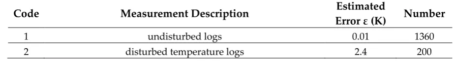
Most of the data used for this case study comes from undisturbed continuous temperature logs (measured when boreholes were at thermal equilibrium), but with only sparse lateral distribution. The accuracy of continuous logs is estimated to be ±0.01 °C [16]. The remaining data are bottom hole temperatures (BHT) or temperature data from drill stem tests (DST). The BHT data have a much larger, and thus in a geostatistical point of view, better spatial (especially lateral) distribution compared to all the other temperature values. However, usually the quality of BHT measurements is rather poor since they are carried out during or shortly after the drilling process when the thermal field around the wellbore is strongly disturbed and thus in disequilibrium. The accuracy of corrected BHT values depends on the number of single measurements per well and the quality of documentation of these measurements and thus the correction method, which can be applied [17-19]. This results in measurement errors of ±3 °C at minimum and up to ±5 °C-10 °C as presumed maximum [16, 20, 21]. However, the real measurement error is usually unknown and could only be quantified by later continuous temperature logging. Based on the quality of the data, a respective measurement error is estimated and shown in Table 1 (for details see [10, 22, 23]).
Table 1. Description of the different subsurface temperature measurements including estimated errors and number of measurements per measurements type for this case study.
Code Measurement Description Estimated
Error ε (K) Number
1 undisturbed logs 0.01 1360
11
Bottom hole temperature (BHT) with at least 3 temperature measurements taken at different times at the same depth;
corrected with a cylinder -source approach
0.5
58
21 Production test or Drill Stem Test (DST) 0.5
12
BHT with at least 2 temperature measurements taken at different times at the same depth; corrected using the Horner
-plot method
0.7
85
13
BHT with at least 2 temperature measurements taken at different times at the same depth; corrected with an explosion
line-source approach
0.7
14 BHT with one temperature measurement, known well radius
and time since circulation (TSC) 1.6 46
15 BHT with one temperature measurement, known TSC 1.6
16 BHT with one temperature measurement, known well radius 3
280 17 BHT with one temperature measurement, unknown well
radius and unknown TSC 3
Figure 2. (a) Generalized geological map of the federal state of Hessen; geology after [24], faults after [25]; (b) submodels within the 3D model, for abbreviations see text; locations and depths of temperature data (modified after [26]) and locations of cross sections; the 22 available logs which are used for validation are marked and numbered.
In this study the global trend value (spatially variable geothermal gradient, see section 2.4) is removed from the data for variogram modeling and the subsequent kriging and finally added to the kriging results again. For the linear regression the surface temperature is assumed to be constant at 5 °C.
2.3. Variograms
A difficult but important part is the derivation of good variograms for the horizontal and vertical direction. The variograms give necessary information about the spatial dependence of the data. The horizontal variogram is based on all data from the Odenwald and Sprendlinger Horst (ODW), Hanau Seligenstädter Senke (HSS), Hessen North-East (NE) and Schiefergebirge/Rhenohercynian (RH) submodels. Data from the Mainzer Becken (MZ) and the Oberrheingraben (ORG) submodels (Figure 2) are not used for this variogram as they are strongly disturbed by convective heat transport processes. The vertical variogram is based on data from all regions but only high quality measurements from continuous logs are used.
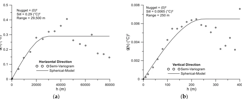
The calculated experimental variograms and the fitted functions are shown in Figure 3. The variograms are calculated based on the residual temperature data where the trend is removed as described above. The result for the horizontal direction is shown in the left of Figure 3. Due to the high geological heterogeneity within and between the combined model units, the result is quite poor, but it is still possible to fit a theoretical variogram to the data.
With the complete data-set it is not possible to obtain a reasonable experimental variogram for the vertical direction. However, if solely the high quality continuous logs are used, with data only from depths larger than 250 m, the result is substantially better (Figure 3 right). As the horizontal distribution of these log data is very sparse it is not possible to calculate a horizontal variogram based on these data only. The vertical variogram shows a clear non-stationary progression from 250 m on, which is neglected for the modeled variogram; at interpolation this is considered due to a search radius limited to 200 m. The fit for the horizontal case is obviously poor. However, a perfect fit is in general not necessary [11]; a qualitative fit is mostly sufficient. The estimated values for the range are comparable to the values estimated by [6] for the Provence basin, of horizontal 23 km and vertical 500 m.
(a) (b)
2.4. Numerical Modelling
A classical approach for estimating the subsurface temperature distribution is the numerical computation of a 3D purely conductive steady state temperature distribution (e.g. [27, 28]).
Based on a 3D structural GOCAD model [29] and an extended geothermal database [26] of the federal state of Hessen/Germany the subsurface temperature distribution is computed. The 3D structural model comprises the model units of Quaternary/Tertiary in a combined unit, the mesozoic Muschelkalk (mainly limestones and marls) and Buntsandstein (sandstones, conglomerates and pelites), the paleozoic Zechstein (limestones, dolomites and evaporites), Permocarboniferous (sandstones, conglomerates, pelites and volcanics) and the Pre-Permian basement. The basement was divided according to the internal zones of the variscan orogen into the Mid-German Crystalline Rise (MGCR) in the southeastern part of Hesse, which mainly consists of felsic granitoids and subsidiary of metamorphics and basic intrusives and the Rheno-Hercynian and Northern Phyllite Zone (RH & NPZ) in the northwest, consisting of low-grade metamorphic pelagic to hemipelagic as well as volcanoclastic source rocks
The 3D finite element mesh with layers for all geological units is constructed by converting the original Hessen 3D GOCAD Model [29]. The model grids have a horizontal resolution of 0.5 km in x and y direction. The vertical height of the elements is adapted to fit the topography of the model units and ranges from 5 to 50 m. The thermal conductivity representing a weighted mean value considering the dominant lithology described in [26] is assigned to the respective model units (see Table 2). The natural petrophysical heterogeneity of the rocks [30] summarized in the model units is for this methodological study not considered in detail, as it would be needed for real resource assessment or reservoir models. The crustal units of the MGCR consisting mainly of granitic to granodioritic rocks (e.g. [31]) and the RH and NPZ consisting of various metasediments (e.g. [32, 33]) were each modelled as homogeneous units without further lithological subdivisions as proposed by [34]. As mentioned above for this purely methodological approach, which was not intended as basis for resource assessment or other following applications no calibration was performed.
On the surface long-term yearly average temperatures (data from the German Meteorological Service, DWD) are assigned as Dirichlet boundary conditions. A basal heat flow is estimated following the approach of [29]. It is spatially varying from 65 mW m-2 to 95 mW m-2 according to the
presumed Moho depth using data from [35]. Using these high values for the simplified approach compared to e.g. [36] means that the radiogenic heat production within the shallower units is assumed to be incorporated in the heat flow and does not need to be regarded as additional internal heat source. The shallowest position of the Moho coincides with the northern Upper Rhine Graben and the Odenwald (ORG and ODW in figure 2). It descends towards the north-west and north-east while it has an SSW-NNE elongated local high following the northeastern prolongation of the Upper Rhine Graben under the Cenozoic Vogelsberg volcano into the Hessian depression, which are illustrated by the Quaternary and Tertiary sediments in the NE model unit in figure 2.
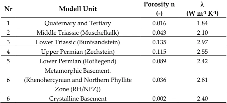
Table 2. Assigned porosity and thermal conductivity values for the units of the numerical model.
Nr Modell Unit Porosity n
(-)
(W m-1 K-1)
1 Quaternary and Tertiary 0.016 1.84
2 Middle Triassic (Muschelkalk) 0.043 2.10
3 Lower Triassic (Buntsandstein) 0.135 2.97
4 Upper Permian (Zechstein) 0.115 2.55
5 Lower Permian (Rotliegend) 0.089 2.42
6
Metamorphic Basement.
(Rhenohercynian and Northern Phyllite Zone (RH/NPZ))
0.036 2.81
(Mid-German Crystalline Rise (MGCR))
Several codes are available for the numerical solution [37]. Here the software FEFLOW [38] was used. Only conductive heat transfer is considered as both not enough data on the hydraulic properties of fault zones and individual model units and on the detailed 3D structure of all relevant fault zones acting as vertical conduits are available for convective heat transport modeling at great depths. The paleoclimatic disturbances of the temperature (e.g. [39]) are also not considered; neither are internal heat sources and the temperature and pressure dependence of the relevant rock properties. Furthermore, we assume an equilibrium situation for the model area and calculate the temperature by solving numerically the conductive heat equation for steady-state conditions. The solution therefore simplifies to:
(
)
=0
λ T (5)
The temperature distribution thus is independent of heat capacity and density but sensitive to thermal conductivity values and to the choice of boundary conditions. This follows observations of [48] which showed that the subsurface thermal field in conductive models is most sensitive to thermal conductivity.
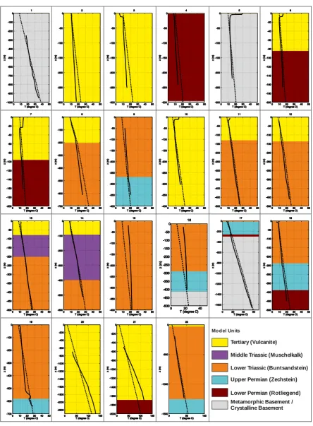
Mo d el Un its
Tertiary (Vulcanite)
Middle Triassic (Muschelkalk)
Lower Triassic (Buntsandstein)
Upper Permian (Zechstein)
Lower Permian (Rotliegend) Metamorphic Basement / Crystalline Basement
Figure 4. Comparison of measured temperatures (straight line) with the conductive modelled temperatures (dotted line). For locations of the logs compare numbers with Fig. 2b. Logs 15, 16, 19, 20 and 21 are presumably affected by convective heat transport processes.
2.5. Kriging with External Drift
estimation of the primary variable. However, the fundamental relation must make sense in terms of the underlying physics.
The trend m(u) is modeled as a linear function of a smoothly varying secondary (external) variable fk, instead of a function of the spatial coordinates, like in kriging with a trend model. fk is
assumed to reflect the spatial trends of the z variability up to a linear rescaling of units. The estimate of the variable and the corresponding system of equations are identical to the kriging with a trend model [40]. Now for the KT estimator the full kriging with trend system can be written as [41]:
(
)
( )
( )
( )
( )
(
( )
)
−
=
−
T k T i T T j k T i k j if
w
f
f
x
x
x
x
x
x
x
x
x
0
(6)fk(x) are secondary data which have to be known for all grid nodes and all observation points. For further details see [40].
Additionally, similar to the ordinary kriging, the measurement error is considered in the study presented here by adding a variance to the main diagonal of the left-hand side matrix.
For this study the same settings like for ordinary kriging have been applied for kriging with external drift; using an extended version of jk3d the result of the numerical model was added as drift variable by interpolating the result to all mesh nodes and data points, by using an inverse distance weighted interpolation.
The KED result showed at some locations at the border anomalous temperatures. For stabilizing the solution several artificial temperatures according to the geothermal gradient were added, but only outside of the solution domain; additionally a very large measurement error of 25 °C is assigned which reduces the impact on the solution further.
3. Results
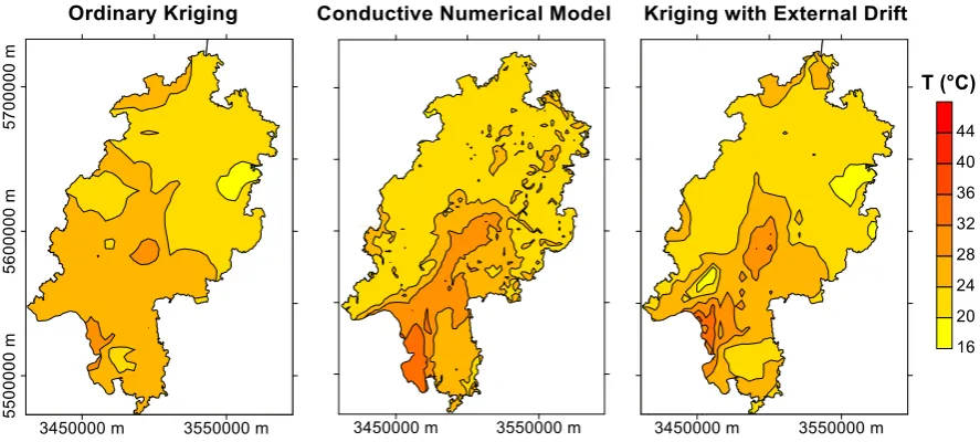
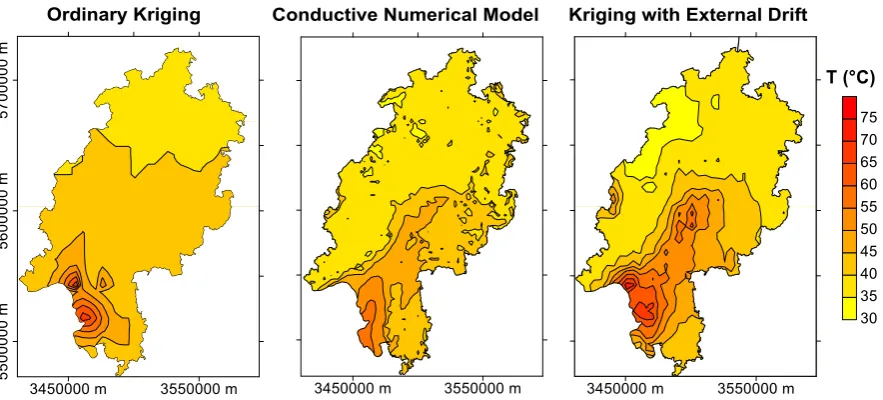
In Figures 5, 6 and 7 the results for ordinary kriging, the conductive numerical model and kriging with external drift are shown for a depth of 500 m, 750 m and 1,000 m below the surface, respectively.
For the ordinary kriging and the kriging with external drift a modified approach is applied where the quality of the temperature measurements is taken into account [10]. Though the data are distributed too sparsely for evaluating the total area using ordinary kriging, no blanking is applied. This makes the comparison with the two other results easier.
Figure 6. Comparison of ordinary kriging, conductive numerical modeling and kriging with external drift results in 750 m depth below the surface.
Figure 7. Comparison of ordinary kriging, conductive numerical modeling and kriging with external drift results in 1,000 m depth below the surface.
Finally, the result of kriging with external drift (figure 5c, 6c and 7c) combines the numerical result with the geostatistical interpolation. This way the subsurface temperature is predicted using all information available and a much better fit of geological subsurface structure and known geothermal anomalies is accomplished.
4. Discussion
While the subsurface thermal field in the northern part of Hessen is dominated by heat conduction, strong thermal anomalies occur in the northern Upper Rhine Graben in the southwest of Hessen. There is a broad consensus that these anomalies are a result of convective heat transport along deep seated fault systems [16, 42, 43]. However, where precisely the hot water comes from - the south following the general topographic gradient of the Upper Rhine Graben or from the graben flanks in the east and west - is still a mainly unanswered question. No regional data of hydraulic heads of depths deeper than say 500 m below the surface exist.
For instance [2, 44] and later [45] favor an explanation where meteoric water on the western and eastern sides of the graben infiltrates the neighboring crystalline formations on the eastern graben border (Odenwald, Black Forest) and on the western border (Vosges, Pfälzer Wald) through deep seated permeable fault systems or zones. This infiltrating water is then descending and heated; in the Mesozoic and Paleozoic bedrock below the graben and then again ascending along the fault systems within the graben and brings the heated water into comparable shallow depth in the vicinity of the river Rhine acting as gaining stream with the lowest regional hydraulic head.
However, several questions are raised by such an argument: the fluids circulating within the deep aquifers in the Rhinegraben are known to be highly mineralized [45] and therefore considerable denser then fresh water – typically this causes stagnation and very high geothermal or hydraulic gradients are needed for upwelling.
Keeping in mind that average hydraulic conductivities of units like the Odenwald crystalline should be in the order of 10-7 m/s or lower (e.g. [46]) flow processes are very slow. Even if faster
transport is possible along preferential vertical flow paths like faults and fractures at the graben main boundary faults, the net amounts of transported fluid are assumed to be considerably small.
[16] suggested that the observed anomalies close to Landau in the Rhine Graben, are a result of south to north directed groundwater flow together with free convection within the graben parallel faults, which causes upwelling of relatively hot water. Given the permeability of the graben sediments and the Mesozoic sediments below including graben parallel and thus mainly north-south oriented faults the flow rate in south-north direction can be expected to be much higher than in east-west direction where the main faults would need to be crossed, which usually act as lateral barriers. In extension of this study [23] showed that fault parallel flow can be forced to upwell at locations where faults intersect. This is also significant for the faults at the northern end of the Upper Rhine Graben and in the vicinity of the city of Wiesbaden and the other known thermals spas along the already mentioned Taunus-Hunsrück-Boundary Fault. All these upwelling locations of thermal water coincide with the intersection of Rhenish (NNW-SSE, N-S to NNE-SSW) and Variscan (WSW-ENE) striking faults. The advantage of the latter explanation is that the effect of free convection, which is hard to predict for such heterogeneous geological environments, is not mandatory anymore.
5. Conclusions
Differences in the predicted subsurface temperature distribution are mainly related to convective processes, which are reflected by the interpolation result, but not by the numerical model. Therefore, a comparison or rather the combination, as presented here, of the two results is a good way to obtain information about flow processes in such great depths. This way an improved understanding of the heat transport processes within the presented low-mid enthalpy geothermal reservoir (500 m – 6000 m) is possible.
hydraulic properties - and missing full understanding of convective (heat transport) along faults (including the coupling of mechanics and hydraulics and the in situ stress field) any such result lacks of reliability and up to now usually fails in predicting convection cells at the right locations.
Obtaining the theoretical variograms necessary for kriging is a difficult task. This is especially true for the poor quality of the horizontal semi-variogram. However, it is sufficient for obtaining a reasonable spatial temperature distribution. By the inclusion of a weighting algorithm [10] the kriging result can be strongly improved as both artefacts due to low quality measurement only have a small impact - where high quality data are available and more data can be used for kriging compared to standard approaches where low quality data usually is neglected.
As demonstrated here, the combination of both approaches results in a temperature model with a good fit to the given temperature measurements as well as a good extrapolation of subsurface temperatures in depths where no data is available. Such a model increases the quality of subsurface temperature predictions compared to purely numerical or geostatistical approaches and thus would allow for more reliable geothermal resource assessment on a regional scale.
In this study the paleoclimate signal was not taken into account, which is especially relevant for depths up to approximately 1,000 m. Also, heat production was neglected for the numerical model. Both aspects as well as the influence of fault zones as conduits for convective heat transport and the influence of mechanics and the orientation to the in situ stress field on fault permeability should be addressed in future work. Additionally the heterogeneity of the reservoir properties as well as the impact of e.g. temperature and or pressure dependent thermal conductivity as well as permeability could be addressed by specific modeling approaches.
Supplementary Materials: The code used for the interpolation (jk3d) is freely available as open source code from https://sourceforge.net/projects/jk3d/.
Acknowledgments: This work is supported by the DFG in the framework of the Excellence Initiative, Darmstadt Graduate School of Excellence Energy Science and Engineering (GSC 1070).
Author Contributions: Wolfram Rühaak. and Kristian Bär conceived and designed the simulations and analyzed the data; Wolfram Rühaak computed the variograms, the numerical simulations and wrote the paper and Kristian Bär contributed the data and knowledge on the geological 3D model, the thermophysical and temperature data and the general geological background of the federal state of Hesse. Ingo Sass internally reviewed the manuscript, made helpful amendments and corrections and thus helped to finalize the manuscript.
Conflicts of Interest: The authors declare no conflict of interest. The founding sponsors had no role in the design of the study; in the collection, analyses, or interpretation of data; in the writing of the manuscript, and in the decision to publish the results.
References
1. Huenges, E.; Kohl, T.; Kolditz, O.; Bremer, J.; Scheck-Wenderoth, M.; Vienken, T. Geothermal energy systems: research perspective for domestic energy provision. Environ. Earth Sci. 2013, 70, 3927–3933. doi:10.1007/s12665-013-2881-2
2. Clauser, C.; Villinger, H. Analysis of conductive and convective heat transfer in a sedimentary basin, demonstrated for the Rheingraben. Geophys. J. Int. 1990, 100, 393–414. doi:10.1111/j.1365-246X.1990.tb00693.x
3. Agemar, T.; Brunken, J.; Jodocy, M.; Schellschmidt, R.; Schulz, R.; Stober, I. Untergrundtemperaturen in Baden-Württemberg. Zeitschrift der Dtsch. Gesellschaft für Geowissenschaften 2013, 164, 49–62. doi:10.1127/1860-1804/2013/0010
4. Bonté, D.; Guillou-Frottier, L.; Garibaldi, C.; Lopez, S.; Bourgine, B.; Lucazeau, F.; Bouchot, V. Subsurface temperature maps in French sedimentary basins: new data compilation and new interpolation. Bull. Soc. Gol. Fr. 2010, 377–390.
6. Garibaldi, C.; Guillou-Frottier, L.; Lardeaux, J.-M.; Bonté, D.; Lopez, S.; Bouchot, V. P. L.. Relationship between thermal anomalies, geological structures and fluid flow: new evidence in application to the Provence basin (southeast France). Bull. Soc. Gol. Fr. 2010, 363–376.
7. Rivest, M.; Marcotte, D.; Pasquier, P. Hydraulic head field estimation using kriging with an external drift: A way to consider conceptual model information. J. Hydrol. 2008, 361, 349–361. doi:10.1016/j.jhydrol.2008.08.006
8. Chilès, J.-P.; Gable, R. Three dimensional modelling of a geothermal field. Geostatistics for Natural Resources Characterization, 1984, Part 2. D, 587–598, Reidel Publish. Comp., Hingbam, MA.
9. Agemar, T.; Schellschmidt, R.; Schulz, R. Subsurface temperature distribution in Germany. Geothermics 2012, 44, 65–77. doi:10.1016/j.geothermics.2012.07.002
10. Rühaak, W. 3-D interpolation of subsurface temperature data with measurement error using kriging. Environ. Earth Sci. 2015, 73(4), 1893–1900, doi:10.1007/s12665-014-3554-5
11. Kitanidis, P.K. Introduction to Geostatistics, Applications in Hydrogeology., Cambridge University Press, Cambridge. 1997
12. Isaaks, E.H.; Srivastava, R.M. An Introduction to Applied Geostatistics. Oxford University Press, Oxford. 1989
13. Chilès, J.P., Delfiner, P. Geostatistics: Modeling Spatial Uncertainty. Wiley, New York. 1999 14. Davis, J.C. Statistics and Data Analysis in Geology. 3rd Edition. Wiley, New York. 2002
15. Delhomme, J.P. Kriging in the hydrosciences. Adv. Water Resour. 1978, 1, 251–266. doi:10.1016/0309-1708(78)90039-8
16. Bächler, D.; Kohl, T.; Rybach, L. Impact of graben-parallel faults on hydrothermal convection––Rhine Graben case study. Phys. Chem. Earth 2003, Parts A/B/C 28, 431–441. doi:10.1016/S1474-7065(03)00063-9 17. Deming, D.Application of bottom-hole temperature corrections in geothermal studies. Geothermics 1989,
18, 775-786, doi:10.1016/0375-6505(89)90106-5
18. Jessop, A.M. Thermal Geophysics. Elsevier, Amsterdam. 1990.
19. Speece, M.A.; Bowen, T.D.; Folcik, J.L.; Pollack, H.N. Analysis of temperatures in sedimentary basins: the Michigan Basin. Geophysis 2012, 50(8), 1318-1334, doi:10.1190/1.1442003.
20. Förster, A. Analysis of borehole temperature data in the Northeast German Basin: continuous logs versus bottom-hole temperatures. Pet. Geosci. 2001, 7, 241–254, doi: 10.1144/petgeo.7.3.241
21. Goutorbe, B.; Lucazeau, E.; Bonneville, A. Comparison of several BHT correction methods: a case study on an Australian data set. Geophys. J. Int. 2007, 170(2), 913–922, doi:10.1111/j.1365-246X.2007.03403.x
22. Rühaak, W. A Java application for quality weighted 3-d interpolation. Comput. Geosci. 2006, 32, 43–51. doi:10.1016/j.cageo.2005.04.005
23. Rühaak, W., Rath, V., Clauser, C. Detecting thermal anomalies within the Molasse Basin, southern Germany. Hydrogeol. J. 2010, 18, 1897–1915, doi:10.1007/s10040-010-0676-z
24. HLUG. Geologische Übersichtskarte Hessen 1:300.000, 5. überarbeitete digitale Ausgabe. 2007 25. Zitzmann, A., 1981. Tektonische Karte der Bundesrepublik Deutschland 1:1.000.000.
26. Bär, K.; Arndt, D.; Fritsche, J.-G.; Götz, A.E.; Kracht, M.; Hoppe, A.; Sass, I. 3D-Modellierung der tiefengeothermischen Potenziale von Hessen - Eingangsdaten und Potenzialausweisung. Z. Dt. Ges. Geowiss. 2011, 162, 371–388, doi10.1127/1860-1804/2011/0162-0371
27. Bayer, U.; Scheck, M.; Koehler, M. Modeling of the 3D thermal field in the northeast German basin. Geol. Rundschau 1997, 86, 241–251. doi:10.1007/s005310050137
28. Scheck-Wenderoth, M.; Maystrenko, Y.P. Deep Control on Shallow Heat in Sedimentary Basins. Energy Procedia 2013, 40, 266–275. doi:10.1016/j.egypro.2013.08.031
29. Arndt, D.; Bär, K.; Fritsche, J.-G.; Kracht, M.; Sass, I.; Hoppe, A. 3D structural model of the Federal State of Hesse (Germany) for geo-potential evaluation. Z. Dt. Ges. Geowiss. 2011, 162, 353–369, doi: 10.1127/1860-1804/2011/0162-0353
30. Cermak, V.; Rybach, L. Thermal conductivity and specific heat of minerals and rocks In: Angenheister, G. (Ed.), Zahlenwerte Und Funktionen Aus Naturwissenschaften Und Technik/ Landolt-Bornstein. Springer, Berlin, Heidelberg, New York, pp. 305–343. 1982.
32. Franke, W.; Haak, V.; Oncken, O.; Tanner, D. Orogenic processes: quantification and modelling in the Variscan belt. Geol. Soc. London, Spec. Publ. 2000, 179, 1–3. doi:10.1144/GSL.SP.2000.179.01.01
33. Stets, J.; Schäfer, A. The Lower Devonian Rhenohercynian Rift – 20 Ma of sedimentation and tectonics (Rhenish Massif, W-Germany) [Das unterdevonische Rhenoherzynische Rift – 20 Ma Sedimentation und Tektonik (Rheinisches Schiefergebirge, Westdeutschland).]. Z. Dt. Ges. Geowiss. 2011, 162, 93–115. doi:10.1127/1860-1804/2011/0162-0093
34. Edel, J.-B.; Schulmann, K. Geophysical constraints and model of the Saxothuringian and Rhenohercynian subductions - magmatic arc system in NE France and SW Germany. Bull. la Soc. Geol. Fr. 2009, 180, 545– 558. doi:10.2113/gssgfbull.180.6.545
35. Dézes, P.; Ziegler, P.A. European Map of the Mohorovičić discontinuity, in: Mt. St. Odile, 2nd EUCOR-URGENT Workshop (Upper Rhine Graben Evolution and Neotectonics), France. 2001
36. Noack, V.; Scheck-Wenderoth, M.; Cacace, M. Sensitivity of 3D thermal models to the choice of boundary conditions and thermal properties: a case study for the area of Brandenburg (NE German Basin). Environ. Earth Sci. 2012, 67, 1695–1711. doi:10.1007/s12665-012-1614-2
37. Anderson, M.P. Heat as a Ground Water Tracer. Ground Water 2005, 43, 951–968. doi:10.1111/j.1745-6584.2005.00052.x
38. Diersch, H.-J.G. FEFLOW: Finite Element Modeling of Flow, Mass and Heat Transport in Porous and Fractured Media, 1st ed. 2014, Springer Heidelberg New York Dordrecht London. doi:10.1007/978-3-642-38739-5
39. Hartmann, A.; Rath, V. Uncertainties and shortcomings of ground surface temperature histories derived from inversion of temperature logs. J. Geophys. Eng. 2005, 2, 299–311. doi:10.1088/1742-2132/2/4/S02 40. Deutsch, C. V.; Journel, A.G. GSLIB: Geostatistical Software Library and Users’s Guide, 2nd Edition. Oxford
University Press, Oxford. 1998
41. Webster, R.; Oliver, M.A. Geostatistics for environmental scientists. Wiley. 2007
42. Clauser, C. Conductive and convective heat flow components in the Rheingraben and implications for the deep permeability distribution. American Geophysical Union 1989, 59–64. doi:10.1029/GM047p0059 43. Lampe, C.; Person, M. Advective cooling within sedimentary rift basins—application to the Upper
Rhinegraben (Germany). Mar. Pet. Geol. 2002, 19, 361–375. doi:10.1016/S0264-8172(02)00022-3
44. Pribnow, D.; Schellschmidt, R. Thermal Tracking of Upper Crustal Fluid Flow in the Rhine Graben. Geophys. Res. Lett. 2000, 27, 1957–1960. doi: 10.1029/2000GL008494
45. Stober, I.; Bucher, K. Hydraulic and hydrochemical properties of deep sedimentary reservoirs of the Upper Rhine Graben, Europe. Geofluids 2015, 15, 464–482. doi:10.1111/gfl.12122
46. Stober, I.; Bucher, K. Hydraulic properties of the crystalline basement. Hydrogeol. J. 2007, 15, 213–224. doi:10.1007/s10040-006-0094-4
47. Schulz, R., Schellschmidt, R.: Das Temperaturfeld im südlichen Oberrheingraben. Geol. Jb., E48, 153-165; Hannover, 1991.
48. Mottaghy, D., Pechnig, R., Vogt, C. The geothermal project Den Haag: 3D numerical models for temperature prediction and reservoir simulation. Geothermics, 40 (3) 2011, 199–210.
![Figure 1. Explanatory diagram of the approach (modified after [7]).](https://thumb-us.123doks.com/thumbv2/123dok_us/7924353.1315773/2.595.89.504.72.389/figure-explanatory-diagram-approach-modified.webp)