Article
1
The Geography of Taste:
2
Using Yelp to Study Urban Culture
3
Sohrab Rahimi 1,*, Sam Mottahedi 2 and Xi Liu 3
4
1 Pennsylvania State University; [email protected]
5
2 Pennsylvania State University; [email protected]
6
2 Pennsylvania State University; [email protected]
7
* Correspondence: [email protected]; Tel.: +1-781-2965152
8
Abstract: This study aims to put forth a new method to study the socio-spatial boundaries by using
9
georeferenced community-authored reviews for restaurants. In this study, we show that food
10
choice, drink choice, and restaurant ambience can be good indicators of socio-economic status of the
11
ambient population in different neighborhoods. To this end, we use Yelp user reviews to distinguish
12
different neighborhoods in terms of their food purchases and identify resultant boundaries in 10
13
North American metropolitan areas. This data-set includes restaurant reviews as well as a limited
14
number of user check-ins and rating in those cities.
15
We use Natural Language Processing (NLP) techniques to select a set of potential features
16
pertaining to food, drink and ambience from Yelp user comments for each geolocated restaurant.
17
We then select those features which determine one’s choice of restaurant and the rating that he/she
18
provides for that restaurant. After identifying these features, we identify neighborhoods where
19
similar taste is practiced. We show that neighborhoods identified through our method show
20
statistically significant differences based on demographic factors such as income, racial
21
composition, and education. We suggest that this method helps urban planners to understand the
22
social dynamics of contemporary cities in absence of information on service-oriented cultural
23
characteristics of urban communities.
24
Keywords: Volunteered Geographic Information (VGI), Yelp, Natural Language Processing (NLP),
25
Machine Learning, Cultural Boundaries, Consumption Behavior, Urban Computation, GIS,
26
Word2Vec
27
28
1. Introduction
29
Socio-economic polarization is a defining characteristic of cities in the global economy [1], [2]. In
30
global markets where economic regulations are minimized, social polarization is an inevitable
31
consequence given the relatively small proportion of the population involved in this growing
32
affluence [3]. In case of the U.S., this social polarization is also ethnic/racial as the prosperous
33
economy in the U.S. was accompanied by massive immigration waves from other countries adding
34
more dimensions to the long-lasting Black and white dichotomy. Not surprisingly, immigrants
35
targeted large cities where most industries were located at and this, in part, led to more diversity in
36
urban population. The multitude of cultural/ethnic groups led to cultural polarization and
37
fragmentation of these global cities where every ethnic group occupied a piece of land [4].
38
Therefore, the American metropolis is plagued by both cultural and economic polarization [3].
39
During the past four decades, the debate over the definition and qualities of urban communities
40
in developed countries grew significantly. Overall, scholars have different opinions regarding the
41
strength of communities. Some believe that the notion of community is lost, some believe it has not
42
changed significantly and other say that it’s been liberated from their constraints [5]. However, many
43
of the recent studies have shown that the liberated hypothesis is more representative of the state of
44
modern communities[5]–[7]. These studies assert that telecommunication and mobility has
45
encouraged dispersed networks of friendship, kinship or communities of interest. Under this
46
condition, the individual’s network is a personal choice that she is free to choose from. Even though
47
telecommunication has facilitated broad networks over space, the spatial segregation instigates sharp
48
borders between communities in American cities. Emphasis on diversity and seeing the city as a
49
melting pot, which is championed by postmodern thinking, has not addressed the gaps between
50
ethnic and economic groups [8].
51
Many studies have attempted to fathom the socio-spatial complexities that emerged in post-war
52
American cities. Most of classic studies of this kind were based on the Census data [9], [10]. Although
53
the U.S. Census data provide valuable information about cities, these data hardly inform us about
54
lifestyles, consumption behavior, cultural factors, and space-use patterns. The past two decades have
55
seen a rapid advancement in the field of urban and social studies partly due to emergence of new
56
crowd-sourced data sources and computation techniques [11]. The new data sources have enabled
57
the researchers to go beyond basic demographics such as race and income and delve into a multitude
58
of socio-spatial phenomena in modern cities. This study aims to contribute to this line of studies by
59
proposing taste as an indicator of social status which integrates different facets of culture, economy
60
and social networks of urban inhabitants. We argue that using businesses as sensors can provide new
61
insight into the intricate social structure of the American metropolis. More specifically, this research
62
aims to answer the following questions:
63
To what extent is taste a good indicator of socio-economic status of communities in American
64
cities?
65
By utilizing the concept of taste, can we use restaurant-as-sensor instead of
citizen-as-66
sensor [12] to examine the socio-economic dynamics of neighborhoods without having the
67
User IDs? This issue is especially important to us since business data is far more accessible
68
and plentiful than individual-level data [13].
69
Are American cities comprised of regions with different dominant taste cultures [4]? Are
70
different regions in every city similar to regions from other cities [2]?
71
2. Materials and Methods
72
2.1 Literature review
73
2.1.1 Previous attempts to define socio-spatial boundaries
74
Recently, many studies have addressed these problems by using heterogeneous data sources
75
that are updated frequently and exist at the scale of buildings or individuals [11]. Some investigate
76
the communities on a large scale. For example, one study used vehicle GPS traces in Pisa, Italy to
77
build a network and used community detection algorithms (i.e. Infomap) to identify non-overlapping
78
communities of people at the county and municipality scale [14]. A similar study was conducted on
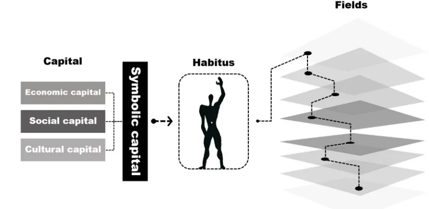
79
a larger scale in Great Britain using telecommunications data [15]. Recently, detecting communities
80
on urban scale has been more popular. For example, one study uses human mobility between
81
region using topic-based inference model [16]. Using this model, this research identifies nine
83
functional regions using clustering techniques.
84
Most often, urban studies that use crowd-sourced data to study the socio-spatial structure of
85
cities incorporate Location-Based Social Network (LBSN) techniques, that is, a network consisting of
86
people in a social structure who share location-embedded information [11] . Much of research in this
87
area uses social media data which includes the geographical location as well as their tagged images,
88
videos, and texts. Common examples of data used for LBSNs include GPS trajectories of taxis,
89
Twitter, Call Data Records (CDRs), Flickr geo-tagged photos, and Foursquare check-in data.
90
Georeferenced crowd-sourced data such as tweets, photos, and check-ins can help understand
91
people’s lifestyles (e.g. likes and dislikes) [17], [18], cities’ socio-spatial structure [19], neighborhood
92
functions and characteristics [20] and behavioral patterns [21] in cities.
93
One of the common techniques for studying urban structure is identifying similarities between
94
users in terms of their use of urban spaces [19], [22]–[25]. For example, among the most well-known
95
studies of this kind is the Livehoods project, which uses check-in data to identify the zones where
96
their establishments (e.g. restaurants and bars) share similar clientele [19]. This study uses 18 million
97
check-ins collected from Foursquare, a location-sharing service where users share their location by
98
checking in via their smart phones. By using clustering techniques, this study identifies clients with
99
similar points of interest (POI). In another study, the authors studied the semantics of different
100
locations by analyzing different categories of POIs in many neighborhoods [25].
101
Although the state of the art techniques used in these studies have dramatically improved our
102
understanding of cities, they still have some limitations. First, accessing data that include individuals’
103
behavior is often hard and these data are not freely available to the public. For example, companies
104
which maintain a great inventory of georeferenced social networks do not share such information
105
due to privacy issues. Second, the data is not often representative of the entire population. For
106
example, not everyone has a Foursquare account and not all those account owners use Foursquare
107
every time they visit a place [19]. Third, these studies only address one aspect of an individual’s life,
108
for example, Foursquare only covers check-in data and points of interest (POIs), and taxi data cover
109
some travel patterns. While these data-sets have proven helpful, multiple data sources need to be
110
fused to provide an understanding of urban lifestyle.
111
112
2.1.2 Taste as an indicator of urban culture
113
The social construct of taste is a well-studied topic especially in the age of Internet where
114
individual preferences are available to information-based companies (e.g. Amazon, Facebook,
115
Spotify). In fact, many recommender systems (i.e. algorithms made for recommending products to
116
users) are designed under the same assumption that people of same social groups are likely to
117
consume similar products [26], [27]. The underlying mechanism of the relationship between social
118
groups and taste was discussed by Pierre Bourdieu in his well-recognized book Distinction: A Social
119
Critique of the Judgment of Taste [28].
120
In Bourdieu’s view, both cultural and economic capital are the most important forms of capital.
121
Economic capital has to do with individuals’ access to economic resources while cultural capital is a
122
Figure 1. Bourdieu’s theory of distinction. Fields refer to different sub-spaces of society such as family groups and
work groups. Individuals’ role in these fields is influenced by her symbolic capital.
views, use of vocabulary, and language skills. Bourdieu believes that taste is the means of identifying
124
class distinction. He argues that these differences are most obvious in the routine everyday choices
125
in taste of food, furniture, and clothing as they are representative of the pure taste. For example, he
126
argues, children of a lower social status like plentiful and good meals while those of higher status go
127
for original and exotic. These choices, according to Bourdieu, become intrinsic to one’s personality
128
and thereon he/she rejects the tastes of other groups. Bourdieu argues that high-taste is characterized
129
by how far it is from pure necessities. The upper classes in this regard use taste as the ideal weapon
130
in strategies of distinction [28].
131
132
133
134
135
136
137
138
139
140
141
142
143
144
145
146
147
Many studies followed Bourdieu’s theory of distinction to determine how demographic factors
148
were correlated with taste. For example, some studies showed that generally, people of higher
149
economic status read more literature and quality papers [29] and have different taste in art [30]. More
150
recent studies on Facebook and MySpace data-sets, argue that people with similar social networks
151
share similar tastes of music, movies, TV shows and books [18], [31]. In all these studies, taste is seen
152
as a means of distinction between different groups of people, which further supports Bourdieu’s
153
argument. According to Bourdieu, individuals may play different roles in different fields of a society
154
(i.e. sub-spaces of society such as friend groups and institutions). The quality of these roles relies
155
heavily on an individual’s symbolic capital, which Bourdieu defines as a combination of social,
156
economic and cultural capital. As discussed earlier, Bourdieu believes that taste best reflects the
157
symbolic capital, which is the main reason of distinction in societies (Figure 1).
158
159
2.1.3 How can information about restaurants help us understand the socio-economic and cultural structure of
160
cities?
161
Businesses are an effective type of sensors that can reflect what is accessible and offered to a
162
neighborhood. Theoretically, it is not surprising to expect geographically concentrated clusters of
163
cities are characterized by highly fragmented social fabric with segregated communities of different
165
taste, culture, ethnicity and economic status. Second, their economies are global and products of all
166
types belonging to all different cultures and nationalities are offered in the marketplace and therefore
167
the consumer is offered a variety of goods from which she can choose [32]. Third, in case of the U.S.,
168
the rise of individualism and diversity along with the economic growth of the post-war period has
169
generated a dominant landscape in cities known as consumption spaces. These spaces gradually took
170
the place of production spaces such as factories after the era of industrialization [33]–[36]. The
171
emergence of these spaces is a result of the increasing impact of consumerism, pushing the
172
individuals towards consuming goods and certain types of services [4], [37]–[40].
173
Restaurants are one of the most common and frequently used consumption spaces. In the U.S.,
174
restaurant expenditures exceed spending in higher education, computers, books, magazines,
175
newspapers, movies and recorded music [41]. Data on consumption behaviors in restaurants is
176
available in different social media venues such as Yelp. Yelp is a web-based application which
177
maintains crowd-sourced reviews of local businesses (i.e. mostly restaurants, coffee shops and bars).
178
Yelp users have generated nearly 127 million reviews for different businesses across the world [42].
179
Here, we used Yelp data to investigate the urban culture in different cities through the concept of
180
taste.
181
182
2.2 Data
183
Two sets of data were used in this research:
184
Data provided by Yelp [43] which includes 11 cities, 8 of which are in North America (i.e.
185
Cleveland, Pittsburgh, Charlotte, Urbana-Champaign, Phoenix, Las Vegas, Toronto, and
186
Montreal). This data includes 4.1M reviews by 1M users for 144K businesses as well as 1.1M
187
business attributes (e.g., hours, parking availability and ambience). For the case of Montreal,
188
of 86,054 reviews 11,284 were in French, as identified through langdetect 1.0.7 package in
189
Python [44]. Since English reviews may not equally represent all Montreal neighborhoods,
190
demographics, and resident population, we considered Montreal as an outlier and removed
191
it from our analysis. For this study we were only interested in restaurants in
English-192
speaking North American metropolitan areas therefore, we filtered out Montreal and
193
Urbana-Champaign (a small city) as well as points that fell out of the metropolitan
194
boundaries. Also, we only used businesses tagged as restaurants. This process resulted in
195
2,186,054 reviews for 34,231 restaurants. This data includes the following fields: Business
196
ID, User ID, Reviews, Business Name, Star Rating, Address, City, State, Zip code, Business
197
Category, Review Count, Longitude, Latitude. The geographic coordinates represent the
198
location of businesses.
199
As we discussed in the introduction section, we intended to see if we can characterize the
200
socio-economic status of urban communities without having information about users. This
201
is very important, because although it is possible to scrape data from different websites such
202
as Yelp, the user IDs are often not provided in the interface and cannot be scraped easily. In
203
other words, extracting information from businesses from the web is often easier than
204
from the web and stripped from user IDs can inform us about neighborhoods, we scraped
206
restaurant reviews and attributes for Boston, Washington D.C., Detroit and Philadelphia
207
metropolitan areas. All these cities are characterized by high segregation as well as ethnic
208
and cultural diversity. This data includes 509,319 reviews for 120,801 restaurants. Using the
209
earlier data-set, we expect to be able to study the communities in this data-set where the
210
user IDs are absent. Also, the four cities are important metropolitan areas and studying the
211
socio-spatial dynamics of these cities can be useful per se.
212
213
214
215
216
2.3 Methodology
217
In using the Yelp data-set, our assumption is that when a person talks about a food or drink in
218
her comment, she has purchased or at least considered that food or drink and therefore, it can be used
219
as an indicator of one’s choice of food or drink. In the following sections we explain our methods for
220
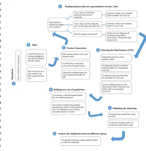
this research. Figure 2 summarizes our work-flow.
221
2.3.1 Feature generation
222
In this study we use the text provided by Yelp reviewers when they post restaurant reviews on
223
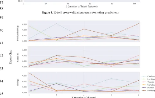
Yelp.com. We use a bag-of-words model to define features for every restaurant. In this model the
224
existence of a word, regardless of the way its embedded in the comment, is considered. A
bag-of-225
words model is suitable for our case, as we are only interested in the frequency of these words and
226
not the way they’re used in the sentence. According to Bourdieu’s theory of distinction, food, drink,
227
and interior decoration are among the best indicators of taste reflecting one’s everyday choice [28].
228
We are, therefore, interested in three categories of features: foods and drinks (e.g. pizza, martini),
229
adjectives used to describe foods (e.g. fried, steamed), and adjectives described for ambience (e.g.
230
rustic, minimalist). We assumed that ambience is an equivalent of decoration. Ambience are among
231
those concepts that are frequently discussed in Yelp reviews along with food, price, and service [45]
232
and provide an overview of the restaurants atmosphere and decorative features such as classy,
233
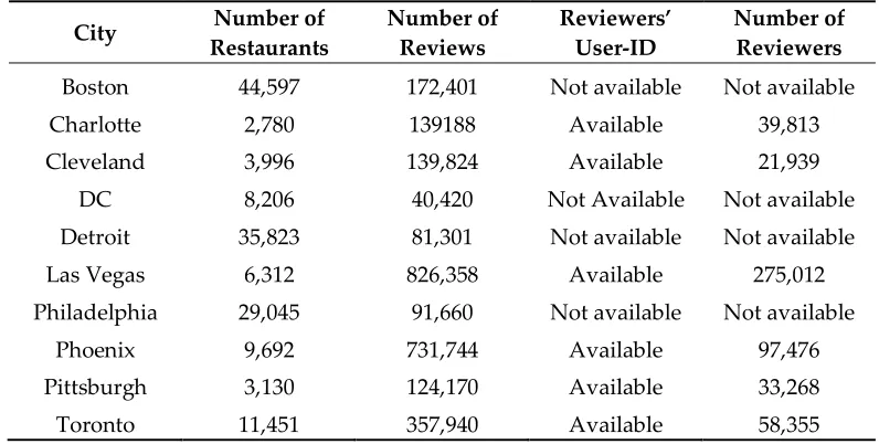
City Number of
Restaurants
Number of Reviews
Reviewers’ User-ID
Number of Reviewers
Boston 44,597 172,401 Not available Not available
Charlotte 2,780 139188 Available 39,813
Cleveland 3,996 139,824 Available 21,939
DC 8,206 40,420 Not Available Not available
Detroit 35,823 81,301 Not available Not available
Las Vegas 6,312 826,358 Available 275,012
Philadelphia 29,045 91,660 Not available Not available
Phoenix 9,692 731,744 Available 97,476
Pittsburgh 3,130 124,170 Available 33,268
Toronto 11,451 357,940 Available 58,355
intimate, romantic, hipster and so forth. In choosing features we avoided selecting words that have
234
multiple connotations or are too general (e.g. nice, green).
235
236
237
238
239
240
241
242
243
244
245
246
247
248
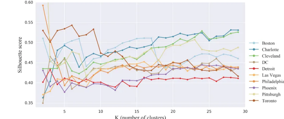
249
250
251
252
253
254
255
256
257
258
259
260
261
262
263
In order to select relevant features from reviews, we used a four-step process:
264
1. first, we used English stop-words to remove commonly-used words [46] and then, chose features
265
among the top 1000 frequent words. Fourty-five features of the three categories (i.e. foods and drinks,
266
food adjectives, and ambience adjectives) were selected at this step (Appendix A).
267
2. Although frequent features can provide much information for restaurants, we expect to get more
268
specific words from the comments. For example, different types of fish (e.g. haddock, tilapia) or
269
different adjectives used to describe an ambience (e.g. divey, hipster) are not among frequent words.
270
To address this problem, we used the Word2Vec model. This open-source model was developed by
271
Google in 2013 which transforms words in a document to high-dimensional spatial vectors by using
272
a Neural Network Language Model (NNLM) [47], [48]. Given N user comments and the n-th word
273
in the comment
w
n, and the window size of the context centered on the n-th word as , the
274
maximum likelihood function of the NNLM model will be as follows:
275
I
(
)=
1
N
i
=1
N
log
p
(
w
n
|
w
n+c nc) (1)
276
Where
w
nn+cc represents a set of words at the center of which isw
n with context sampling277
window size of c. Word2Vec suggests two mathematical frameworks for solving Equation (1) i.e.
278
Continuous Bag-of-Words (CBOW) and Skip-Gram. In summary, Skip-Gram uses stochastic
279
processes to sample from the words whereas CBOW offers a continuous input and training
280
mechanism. In this study, we use CBOW to train the model as some studies suggest it has a better
281
performance at characterizing the words [Error! Reference source not found.]. We trained our Yelp
282
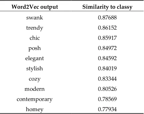
corpus with this model and every word was turned into a 100-dimensional vector. As an example,
283
Table (2) shows the closest words to the word classy. It is noteworthy that the model does not
284
necessarily return synonyms of classy but rather, it considers the way word classy is used in a
285
sentence and therefore, it returns all adjectives that are used to describe an ambience. The 45 words
286
chosen in the last step were given as input to this model to find the 20 closest words in cosine distance.
287
However, not all these 20 words were relevant to food, drink, or ambience. Accordingly, we went
288
through all the 900 words (i.e. 45*20) and selected related words subjectively. It is important to note
289
that Word2Vec model significantly simplified the filtering process and instead of going through all
290
the words in the corpus, we just went through the Word2Vec outputs that is 900 words total. At the
291
end of this step, a total of 454 features were selected.
292
293
Table 2. Top 10 most similar words to classy
294
295
296
297
298
299
300
301
Word2Vec output Similarity to classy
swank 0.87688
trendy 0.86152
chic 0.85917
posh 0.84972
elegant 0.84592
stylish 0.84019
cozy 0.83344
modern 0.80526
contemporary 0.78569
302
3. We binarized the number of words selected from the last step in each comment (1 word exist 0
303
otherwise) and aggregated them for every restaurant. Given that these words are not equally
304
common we use Term Frequency-Inverse Document Frequency model (TF-IDF) to weight these
305
features:
306
307
308
idf
(
t
,
D
)=
log
N
1+|{
d
D
:
t
d
}|
(2)
309
Where N is the total number of restaurants in the corpus and |{
d
D
:
t
d
}| is the number of times
310
that term t appears in the restaurant d. We can then multiply IDF by the Term Frequency (TF) that we
311
previously generated. After this step, for every restaurant, we will have 454 features that are properly
312
weighted.
313
4. The features generated in the previous steps can sometimes fall into categories which can be
314
even more important than the individual features themselves. For example, specific fish types (e.g.
315
salmon) might be important but less informative than the combination of all types of fish. This
316
information tells us that seafood is popular in a certain area. Appendix B indicates the groups of
317
features that we combined in order to generate new features. By including these new features, a total
318
of 477 potentially-unnecessary features remain (e.g. does the word "water" really explain anything
319
about a community’s taste?). In the next step, we explain our methodology for reducing the
320
dimensionality and choosing the most important features.
321
322
2.3.2 User’s taste and the curse of dimensionality
323
In the feature generation process, we took an inclusive approach and considered all features that
324
could possibly represent user taste. Considering all these features for clustering is problematic due
325
to high dimensionality. It is also unclear whether these features represent people’s taste. In other
326
words, we are interested in a subset of features that distinguishes between different groups of users
327
in terms of their practiced taste. For example, the word water may be used equally in all restaurants.
328
In this case, considering water not only doesn’t add any additional information about different
329
neighborhoods but also increases the dimensionality. Therefore, it is important to only select those
330
features that have to do with people’s taste.
331
Recall that the data-set provided by Yelp includes User IDs as well as user-generated ratings for rated
332
restaurants. This data can assist us to select a subset of the 477 features that actually has to do with
333
users’ taste of food, drink, and decoration. Therefore, we examined three scenarios to select the best
334
features related to taste:
335
1.
Users’ choice of restaurant represents their taste for food, drink and decoration:
Under this
336
assumption, a person’s taste is only reflected in the type of restaurants she chooses to visit.
337
Therefore, if we find clusters of restaurants that have been visited by similar users, we should
338
be able to find distinguishing features between these clusters. To this end, we first create a
339
matrix for every city showing whether a user has visited a restaurant (1) or not (0). We generate
340
to restaurants in the same city. By separating the cities, the effect of geography is minimized
342
and we can draw our focus on the effects of restaurant attributes on users’ choice of restaurant.
343
Of all the 525,863 Yelp reviewers, 311,866 reviewers have provided only one review. We
344
removed users with only 1 review since first, these reviews are more likely to be biased and
345
have extremely high or low ratings and we will use the ratings in the next steps. Second,
346
excluding these would reduce the computational costs and also increase the accuracy of our
347
clustering, which we will explain in the next steps. From these matrices, we generated a
348
pairwise similarity matrix using cosine distance:
349
cos(
A
,
B
)=
AB
|
A
||
B
|
=
i
=1
n
A
iB
i
i
=1
n
A
2i
i
=1
n
B
i2(3)
350
Where restaurant A and restaurant B are n dimensional vectors with n being the number of
351
Yelp users in each city. Every element of A and B is 1 if a given user has reviewed that
352
restaurant and 0 otherwise.
353
In the next step, we used spectral clustering [49] to first find the restaurants with similar
354
clientele. This method constructs a graph from the similarity matrix, where the data points (i.e.
355
restaurants) are the nodes and the similarity between them are presented as weighted edges.
356
The algorithm finds partitions of the similarity matrix by detecting low-weight edges. More
357
specifically, this algorithm first performs a dimensionality reduction and then applies a
k-358
means clustering [50] on the low-dimensional embedding. To reduce the dimension, the
359
algorithm first generates a Graph Laplacian L [51]:
360
361
L
=1
D
1W
(4)
362
Where D is the degree matrix with diagonal terms
d
i
=
j
=1
n
W
ij
,
and W is the adjacency363
weight matrix of an undirected graph. The Laplacian matrix L, in fact, is used to calculate the
364
eigenvalues for the matrix. The k-means clustering will then be applied to these eigenvalues,
365
which represent an image of the similarity matrix in a lower-dimension space. Since the
k-366
means is applied to a reasonably lower dimension, the resulting clusters are expected to be
367
more distinguishable and informative. To ensure an optimal number of clusters, we use
eigen-368
gap heuristic method [49] to find the largest difference between two consecutive eigenvalues
369
of the Laplacian matrix and set the number of clusters equal to the rank of the eigenvalues.
370
The check-in row in figure (4) shows the resulting eigen-gaps for different number of clusters.
371
As we can see, for Pittsburgh for example, 2 is the best number of clusters for the check-in
372
matrix.
373
We then select the k best features (from those 477 features) that affect the membership status
374
of a restaurant in one of those previously defined clusters. In other words, we discover which
375
subset of the 477 features actually distinguishes between the clusters using a Deep Feature
376
model used in this study has the following network structure{4774772566416}
378
with a softmax output layer. The first one-to-one linear layer w, between the input layer and
379
the first hidden layer with linear activation function is regularized using an elastic-net [53].
380
The resulting sparse one-to-one layer weights w only selects those features corresponding to
381
none-zero terms in w. The model parameters are learned by minimizing this equation (5).
382
383
384
385
386
387
388
389
390
where
l
(
) is the log-likelihood of the data, the matrix
W
(k) is the kth hidden layer weights391
and
1,2
[0,1]
is the parameter that controls the sparsity of w and the term
1,2is
392
another elastic-net like term that reduces the model complexity and increases the speed of
393
optimization.
394
To find the best subset of features, we tuned hyper-parameters
1,2 and
1,2395
corresponding to the sparsest model with the highest prediction accuracy measured using
F
1396
score which is a weighted harmonic mean of the precision and recall metrics described below:
397
398
recall
=
TP
TP
+
FN
and
precision
=
TP
TP
+
FP
(6)
399
F
1
=2
precision
recall
precision
+
recall
(7)
400
Where TP, FP and FN stand for true positive, false positive and false negative respectively
401
[54]. Since the data for each city is moderately small, 10-fold cross-validation was performed
402
to prevent over-fitting to the training data set.
403
404
2. Users’ choice and the rating they provide both affect their taste for restaurant: The only
405
difference between this hypothesis and the first one is that the rating that one provides for a
406
restaurant acts as a weight to the check-in matrix from the last hypothesis. Accordingly, in this
407
hypothesis, not all restaurants visited by the user are equally important, but rather, we assume
408
those that the user rates higher are more important in determining one’s taste.
409
410
3. Only the users’ ratings determine their taste: In the second assumption we assumed that
411
taste is reflected in the way people rate a restaurant. The only difference here from the last
412
assumption is that we try to see what would happen if every user rated every restaurant. Under
413
this assumption, however, a problem arises: the rating matrix is sparse and many ratings for
414
many restaurants are missing. Using the original rating matrix cannot help us identify how
415
would every user like every restaurant. Therefore, we will need to predict the ratings by using
416
matrix factorization method [55]. The fundamental assumption of this method is that there are d
417
latent features in restaurants that affect the users’ ratings. The advantage of this method is that
418
without having to know what those d features are; we can predict how users might rate
419
restaurants which they have not yet reviewed. We use Singular Value Decomposition (SVD)
420
method to factorize the rating matrix [56]. To find the best number for d, we used 10-fold cross
421
validation. The results indicate that there are approximately 20 latent features (d=20) that affect
422
one’s rating for a restaurant. The Mean Square Error (MSE) decreases significantly up to d=20
423
and gradually increases afterwards due to being over-fit (figure 3). After predicting the rating
424
matrix with 20 latent features for every city, we repeat the steps described in the last two
425
hypotheses. In all three hypotheses above, we selected the number of clusters with the largest
426
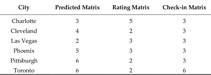
eigen-gaps (figure 4) for every city. Table 3 shows the final number of clusters selected for
427
different matrices and different cities.
428
429
430
431
432
433
434
435
436
437
438
439
440
441
442
443
444
445
Figure 3. 10-fold cross-validation results for rating predictions.
Figure 4. Eigen-gaps for different number of clusters and different
446
447
448
City Predicted Matrix Rating Matrix Check-in Matrix
Charlotte 3 5 3
Cleveland 4 2 3
Las Vegas 2 3 3
Phoenix 5 3 3
Pittsburgh 6 2 3
Toronto 6 2 6
449
2.3.3 Defining the spatial bins
450
451
The features generated from the previous steps reflect Yelp reviewers’ preferences in different
452
urban areas. We next aggregate restaurant features on some spatial units which represent the urban
453
fabric to ensure that nearby restaurants will belong to the same spatial bin. Aggregating restaurants
454
on geographic units will enable us to minimize the impact of outliers and noise. It also enables us to
455
get an overall sense of taste preference given all different types of restaurants in a region. Since our
456
sensors are restaurants, we define these geographical units based on their density and configuration
457
and avoid using administrative boundaries e.g. block groups. Two sets of spatial bins are required to
458
answer our research questions:
459
1. Large-grained spatial bins: These spatial bins enable us to compare different parts of cities
460
together as to see how different cities interact in terms of food, drink, and decoration related
461
attributes. The existing administrative boundaries are too small for this purpose. For example, we are
462
looking at dividing up Washington DC to 3-6 parts and conventional administrative boundaries are
463
too fine-grained for this purpose. Also, we intend to have reasonable spatial bins that are actually
464
representative of the city form. The number of these bins are actually a matter of preference, however,
465
for visualization and simplification purposes we choose large-grained clusters. Accordingly, we use
466
k-means clustering on the restaurants’ geographic coordinates to find reasonable spatial clusters. To
467
find the best number of clusters for each city, we use the silhouette scores [57] for different number
468
of clusters for every city. Silhouette score measures the extent of tightness and separation for each
469
cluster. In other words, it specifies which objects are within their clusters and which ones are
470
somewhere in between:
471
472
( ) =
( ) − ( )
max { ( ), ( )
473
474
Table 3. Selected number of clusters for different matrices and cities
where
a
(
i
)
is the average dissimilarity of datumi
with all other data points andb
(
i
) is the lowest
475
average dissimilarity of i to any other cluster. We then average
s
(
i
) over all data points, a measure
476
that we used for goodness of clustering. Silhouette score ranges from -1 to 1, where 1 means that the
477
clustering configuration is appropriate. Figure 5 shows the Silhouette scores when we divide each
478
city to less than 30 clusters. At this point, we make a compromise between the number of restaurants
479
in every city, area of the city as well as the Silhouette score.
480
481
482
483
484
485
486
487
488
489
2. Small-grained spatial bins: To validate the results and compare it with other demographic
data-490
sets, more fine-grained spatial bins are needed. Administrative boundaries are not helpful in this case
491
either since these boundaries do not consider the formality of the built environment. For example,
492
restaurants located on the Woodward Ave and East 9 Mile Rd cross section in Detroit, MI have been
493
divided between four Census tracts, whereas they are all located near the same cross section and are
494
very close to one another. Another problem with the administrative boundaries is that their sizes are
495
not consistent with the distribution of the restaurants. For example, as we move to the suburbs of
496
Detroit we can see tracts which contain one or two restaurants in them. Accordingly, same as the last
497
step, we use k-means clustering and Silhouette scores to define these spatial bins. This method
498
enables us to consider for the distribution of restaurants while defining the spatial bins. Figure 6
499
shows the Silhouette scores for the four cities. As we can see, for all these cities the Silhouette score
500
improves as we increase the number of clusters. At this point, Silhouette scores are not useful for our
501
purposes as they do not suggest any optimum number of clusters. Therefore, we base our decision
502
on the number of restaurants and city area. Given the number of restaurants we have for every city
503
(table 1), we expect about 200 clusters for Washington D.C., 500 for Detroit and Philadelphia and 600
504
for Boston. It is important to note that there are more census tracts in these areas than the number of
505
clusters that we determined. For example, Detroit metropolitan area has 909 census tracts however,
506
as discussed earlier, due to the uneven spatial distribution of restaurants, our spatial bins are larger
507
than census tracts in the suburban areas with low number of restaurants, but smaller than
block-508
groups in the city centers. It is important to note that the size and number of these spatial bins can
509
change depending on one’s research question as well as spatial resolution of the original data-set (i.e.
510
Yelp in this case).
511
512
513
514
515
516
517
518
519
We use the small-grained and large-grained spatial bins defined in the last step in two different
520
ways. The small-grained clusters are for validation purposes. Our purpose is to see if we can find any
521
clear spatial pattern by clustering these fine-grained clusters. Using small bins enables us to assess
522
the accuracy of this method and compare it with other high-resolution data sources. We will first
523
average the selected set of features from the last step on these spatial bins, scale the features using
524
min-max scaling for every bin, and then calculate the pairwise cosine similarity between the
fine-525
grained bins separately for every city which we didn’t have information about user IDs (i.e.
526
Philadelphia, DC, Detroit, Boston), using formula 3. To calculate the similarities, we will use principal
527
components instead of the actual features, to further reduce the dimension and improve the
528
clustering results. For every resulting matrix, we will use spectral clustering method [58] as described
529
in section 3.2. We will then overlay the resulting clusters on the block-group level map of 2017 income
530
per-capita provided by Tableau 10.0 software for those four cities. At this point, we expect to see a
531
geographic pattern in our clustering as well as a reasonable alignment between the clustering results
532
and the block-group income per-capita layer.
533
After validating, we can use the selected set of features from the last steps to study the
534
interactions between different regions in cities. It is important to note that this capacity is the
535
advantage of this set of features over using user ID data since, at this point, this feature set only relies
536
on the aggregated comments for every restaurant and not the users’ check-ins and ratings. To this
537
end, we will average these features on the large grained clusters, calculate the pairwise similarities
538
and cluster, same as the last step. Due to the extreme cultural, economic, and racial divisions in the
539
American metropolis [4][59] we expect to see different clusters in every city and due to the global
540
nature of these cities [60] we expect some regions from some cities to be similar to other regions in
541
another cities.
542
543
3. Results
544
3.1. Selected features
545
We took the steps described in section (2.3.2), to reduce the dimension of the data set and only
546
focus on those features that are actually representative of users’ choice of food, drink and ambience.
547
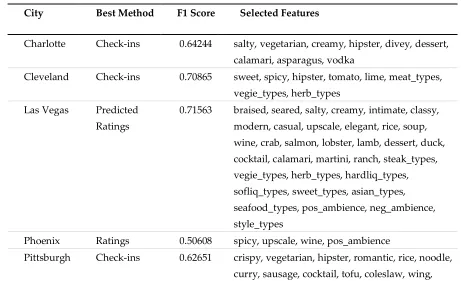
Figure 7 shows the resulting F1 scores for the three hypotheses (i.e. check-ins, ratings, and predicted
548
ratings) and the 6 cities where the user IDs were available (table 1). For every city we selected a taste
549
scenario that returned the highest F1 score. The resulting features along with the scenarios that
550
returned the highest F1 scores, as well as the F1 scores are presented for every city in table 4. By
551
considering all these features, we will have a total of 105 features which we call the Universal Feature
552
Set (UFS). We can now use the UFS to study those cities where the user data is not available. The
553
underlying assumption here is that the 6 cities that we have based the UFS on, are diverse enough
554
that cover the types of food, drink and ambience that one expects to find in the four other cities where
555
the user IDs are not available.
556
557
558
559
560
561
562
563
564
565
566
567
568
569
570
571
572
573
574
575
City Best Method F1 Score Selected Features
Charlotte Check-ins 0.64244 salty, vegetarian, creamy, hipster, divey, dessert,
calamari, asparagus, vodka
Cleveland Check-ins 0.70865 sweet, spicy, hipster, tomato, lime, meat_types,
vegie_types, herb_types
Las Vegas Predicted Ratings
0.71563 braised, seared, salty, creamy, intimate, classy, modern, casual, upscale, elegant, rice, soup,
wine, crab, salmon, lobster, lamb, dessert, duck, cocktail, calamari, martini, ranch, steak_types, vegie_types, herb_types, hardliq_types,
sofliq_types, sweet_types, asian_types, seafood_types, pos_ambience, neg_ambience,
style_types
Phoenix Ratings 0.50608 spicy, upscale, wine, pos_ambience
Pittsburgh Check-ins 0.62651 crispy, vegetarian, hipster, romantic, rice, noodle,
curry, sausage, cocktail, tofu, coleslaw, wing, Figure 7. F1 scores resulting from classification for different cities
3.2 Clustering results
576
Results derived from clustering the small-grained spatial bins with the selected set of features
577
reveal clear geographic patterns which correspond with block-level per-capita income for the four
578
cities where the user IDs were absent (figure 8). We set the number of clusters on two (k=2) for the
579
ease of comparison.
580
581
582
583
584
585
586
587
588
589
590
591
592
593
594
595
596
597
598
599
600
601
602
603
604
605
606
607
608
609
610
611
612
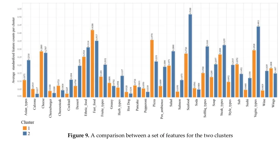
The difference between the type of tastes practiced between the two clusters is shown in figure
613
9. This figure shows the top 30 features with highest average difference between the two clusters. As
614
we can see, features such as seafood, salad, ethnic foods, vegetables, fruits, and Asian food types
615
cheesesteak, lettuce, provolone, ranch, fast_food, dressing_types, pos_ambience, style_types
Toronto Ratings 0.72686 fried, Chinese, salty, Asian, Japanese, steamed, oily, hipster, rice, beer, soup, pork, shrimp, wine,
tea, noodle, seafood, cocktail, sashimi, soy, squid, milk, sesame, Fanta, meat_types, softliq_types,
Asian_types, soda_types, seafood_types, ethnic_food
Figure 8. Clustering results overlaid on per-capita income map for four cities. As we
Figure 9. A comparison between a set of features for the two clusters
show higher values in high-income communities whereas the low-income cluster shows higher
616
consumption of fast food.
617
618
619
620
621
622
623
624
625
626
627
628
629
630
631
632
633
634
635
636
637
638
The fact that this spatial distribution has been derived from small spatial bins indicates the high
639
accuracy of taste as indicator. These maps show that income can be an important factor in
640
determining a communities’ taste. To see empirically how our clusters, correspond with demographic
641
factors, we considered racial composition, educational status, and annual household income at the
642
block-group level for the four cities. Block-group level data is the highest spatial resolution available
643
on Census for these demographics. The data was collected from the American Community
644
service(ACS) website [61]. We defined educational ratio as the ratio of population that have a
645
bachelor degree or higher, in each block-group. The racial composition was defined as the population
646
ratio of Black/A.A., White, and Asian for different block-groups. The income variable is the annual
647
household income in U.S. Dollars. All these demographic factors were estimates provided by the ACS
648
for 2016. We spatially joined the restaurants to the block-groups and conducted t-tests to evaluate the
649
extent to which our clustering results compare with these demographic factors. Table 6 provides a
650
summary of the results. As we can see, the two clusters show significantly different demographic
651
features in all four cities. Looking at all four cities together, we can see that education is the most
652
different demographic factor between the two clusters. Considering the restaurants in all four cities,
653
we can see that education and the Asian population ratio are the most distinctive factors with the
654
highest T-statistics. As we consider each city individually, we can see that the order of importance
655
for different demographic factors differs among different regions. For example, in Boston, the top
656
Cluster Boston, MA Detroit, MI Philadelphia, PA Washington, D.C.
Cluster 1 16,827 17,226 13,849 2,780
Cluster 2 27,770 18,597 15,180 5,419
Table 6. T-test results between the two clusters for demographic variables
distinctive factors are education and Asian population ratio whereas in Washington D.C. the Black
657
population ratio and annual household income have the highest T-statistics. It is important to note
658
that all the four cities show clear spatial boundaries separating the two clusters. In other words, this
659
method proves to be capable of identifying spatial segregation patterns that may have different
660
demographic reasons in different regions (e.g. education level and Asian population in Boston, MA
661
versus income and Black/A.A. population ratio in Washington D.C.).
662
663
664
665
666
City Factor Mean value
in cluster 1
Mean value in cluster 2
T statistic
(absolute value) P value Boston, MA
Educated population ratio 0.06 0.10 97.46 0.000
Annual household income (USD) 66985.93 68655.57 5.47 0.000 Black/A.A. population
ratio 0.41 0.40 13.49 0.000
White population ratio 0.53 0.56 32.97 0.000
Asian population ratio 0.02 0.07 73.04 0.000
Detroit, MI
Educated population ratio 0.04 0.07 59.39 0.000
Annual household income
(USD) 50359.52 61600.40 40.69 0.000
Black/A.A. population
ratio 0.41 0.38 21.84 0.000
White population ratio 0.55 0.60 35.75 0.000
Asian population ratio 0.01 0.03 43.08 0.000
Philadelphia, PA
Educated population ratio 0.05 0.09 72.51 0.000
Annual household income
(USD) 55067.55 64436.73 25.42 0.000
Black/A.A. population
ratio 0.39 0.35 24.14 0.000
White population ratio 0.55 0.62 41.79 0.000
Asian population ratio 0.03 0.05 33.30 0.000
Washington, D.C.
Educated population ratio 0.11 0.15 25.48 0.000
Annual household income
(USD) 53222.42 80220.32 28.74 0.000
Black/A.A. population
ratio 0.36 0.22 41.42 0.000
White population ratio 0.55 0.68 23.94 0.000
Asian population ratio 0.02 0.04 15.19 0.000
All four cities combined
Educated population ratio 0.06 0.09 134.74 0.000
Annual household income (USD) 57322.86 66673.53 51.06 0.000
Black/A.A. population ratio 57322.86 0.37 29.46 0.000
White population ratio 0.40 0.60 69.42 0.000
Figure 10 illustrates the clustering result with 5 clusters for Boston, MA. In this case, as well, we
667
can see clear geographic patterns. For example, we can see orange and green points are both clustered
668
together around the low-income areas. By overlaying these clusters on the African American
669
population, we can see that most of the green points are located in areas with high concentration of
670
African American population. On the other hand, many purple points are located at areas with high
671
income and high concentration of African Americans. This issue gets to the heart of Bourdieu’s
672
argument [28], that taste as an indicator of social status, is not merely a construct of economic capital,
673
but rather it’s derived from symbolic capital, which is in turn, a combination of social, cultural and
674
economic capitals. Accordingly, using taste as an indicator of symbolic capital can shed light on
675
different aspects of communities’ lifestyles which may not be explained similarly with conventional
676
demographic indicator (e.g. income, race) for different geographic and cultural contexts.
677
678
679
680
681
682
683
684
685
686
687
688
689
690
691
692
693
694
695
696
697
698
699
700
701
702
703
Having set our new indicator, we can now use this indicator to study the socio-economic
704
interactions between different regions in different cities. We use the large-grained spatial bins that
705
we previously defined for all cities and choose 5 clusters for simplification purposes (figure 11). The
706
results are consistent with our understanding of global cities. American cities are comprised of
707
spatially separated cultural groups [4]. We can also see that the distribution of these cultural clusters
708
is consistent with our knowledge of some cities. For example, we know that the racial and economic
709
segregation pattern for Phoenix, Pittsburgh, and Washington D.C. approximately corresponds with
710
our results. In some cases, the clusters do not necessarily match with racial and economic measures
711
of those regions. For example, the north-eastern side of Phoenix is in the same cluster as downtown
712
Cleveland while the two regions are demographically different. The earlier is dominantly white and
713
high-income whereas the latter is a low-income mixed-race region. Another anomaly is Toronto
714
which seems to have all its regions in the same cluster colored in cyan. Clusters shown in cyan signify
715
high-income multicultural areas with a variety of restaurant types and cultural groups. This issue
716
might be due to the fact that Toronto does not suffer from extreme racial and economic segregation
717
as is the case for American metropolitan areas [62].
718
719
720
721
722
723
724
725
726
727
728
729
730
731
732
733
734
735
736
737
738
739
740
741
742
743
744
745
746
747
748
749
750
751
4. Conclusion
752
In this study we first used Google Word2Vec model to generate a total of 477 features pertaining
753
to foods, drinks, food qualities, and the interior ambience of restaurants. We extracted these features
754
for the 6 metropolitan areas where the User IDs of the reviewers were available (i.e. Toronto, Phoenix,
755
Las Vegas, Pittsburgh, Cleveland, Charlotte). We then hypothesized three possible scenarios for
756
defining taste and limiting the number of features to those that have to do with users’ behaviors: first,
757
taste may be seen as the combination of factors that encourages a Yelp user to visit a place. Second,
758
the rating that the user gives to a place is also a factor in determining one’s inclination towards a
759
restaurant. Third, the predicted rating of every user for every restaurant should be used as a basis for
760
an individual’s taste. For every one of the matrices generated from these hypotheses, we used the
761
eigen-gap heuristic method to find the best number of clusters. We then solved a classification
762
problem by incorporating the Deep Feature Selection (DFS) model for every hypothesis to see what
763
would be the best subset of those 477 features (i.e. returns the largest F1 score) if we used the clusters
764
defined from the last step class labels. We repeated this process for every one of the 6 cities and for
765
every city we chose the highest F1 score derived from the three hypotheses (Section 2.3.2). We named
766
the union of these 6 sets of features (i.e. one set of features for every city) as the Universal Feature Set
767
(UFS) which became the basis for clustering the cities where the User ID for reviews were absent.
768
By overlaying the clusters identified using the UFS for the four cities with absent user IDs on the
769
2017 block-group level income per-capita map, we showed that our definition of taste can be used as
770
an indicator for studying the socio-economic structure for the four cities where we didn’t have the
771
user IDs. We found a clear alignment between areas of low-income and high-income and our clusters
772
for all the four cities (figure 8). We also showed statistically that the two clusters are significantly
773
different based on different demographic factors representing income, education and racial
774
composition. We showed that education is the most distinctive factor between the two clusters once
775
we consider all four cities combined. We also showed that the two clusters in different cities, while
776
forming clear spatial boundaries, are different in terms of demographic differences between the two
777
clusters. For example, We found that Education and Asian population ratio are the most distinctive
778
factors in Boston while in case of Washington D.C., Black/A.A population ratio and Annual
779
household income are the main distinctive factors.
780
Once we increased the number of clusters we still observed a geographic pattern (figure 10)
781
which results from a combination of demographic factors such as race and income. This issue reflects
782
the multifaceted nature of taste as argued by Bourdieu nature of taste [28]. We showed that this
783
method also works well for more than 2 clusters, although the performance of this method depends
784
highly on the quality of data and number of reviews. Lastly, we used UFS to study the inter-regional
785
similarities for 10 North American cities. Our results showed that all the 9 American cities were
786
comprised of regions that are less similar to one another and more similar to some regions in other
787
cities. This observation is close to our understanding of the global cities as described in the
788
literature [4]. In case of Toronto, all the spatial bins were in the same cluster which might be due to
789
the fact that extremely disadvantaged neighborhoods for different racial groups do not exist
790
compared to the U.S. metropolitan areas [62].
791
As discussed earlier, we do not expect to see a direct relationship between clusters derived from
792
taste and racial and economic segregation patterns in all cultural and geographic contexts: First,
793
commonly used foods and drink in a White community in one city might be quite popular in the
794
African American communities in another. From a theoretical point of view, the taste index assists us
795
to see cities regardless of their mere economic and racial composition, but rather the symbolic capital
796
of the inhabitants which results from social, economic, and cultural capital, combined. Second,
797
reviews provided by Yelp users in a region might not have necessarily been authored by the residents
798
of that region. It is not surprising to see that a considerable number of reviews in downtown
799
Cleveland, for example, have been authored by visitors who do not reside in that region. This issue