Abstract: Characterization the 3-D structure of clouds is needed for a more complete
understanding of the Earth's radiative and latent heat fluxes. Here we develop and explore a “ray casting” algorithm applied to the Multi-angle Imaging SpectroRadiometer (MISR) on board the Terra satellite, to reconstruct 3-D cloud volumes for observed clouds. The ray casting algorithm is first applied to geometrically simple synthetic clouds to show that, under the assumption of perfect, clear-conservative cloud masks, the reconstruction method yields overestimation whose magnitude depends on the cloud geometry and the resolution of the reconstruction grid relative to the image pixel resolution. The method is then applied to two select MISR scenes, fully accounting for MISR’s viewing geometry for reconstructions over the Earth’s ellipsoidal surface. The MISR Radiometric Camera-by-camera Cloud Masks at 1.1 km resolution and custom cloud masks at 275 m resolution independently derived from MISR RGB channels are used as input cloud masks. A wind correction method, termed “cloud spreading”, is devised and applied to the cloud masks to offset potential cloud movements over short time intervals (around 7 minutes at maximum) between the cameras. The MISR cloud top height product is used as a constraint to reduce the overestimation at the cloud top. The reconstruction results show that their uncertainty is significant when the wind correction is applied, and that they have more refined structures when the input cloud mask has a higher resolution. Recommendations for improving the presented cloud volume reconstructions as well as for future passive remote sensing satellite missions are discussed.
Keywords: MISR; cloud volume; cloud geometry; cloud shape; cloud boundary; cloud volume reconstruction.
1. Introduction
Characterizing 3-D cloud structures, such as shape, altitude, and volume, is critical in understanding the distribution of the radiative fluxes and latent heat fluxes on the Earth [e.g., 1, 2]. Compared to the traditional 1-D or 2-D treatments, the 3-D cloud structures have a distinguishing impact on not only the forward calculations of the fluxes (e.g. [3-6]), but also the inverse problem of retrieving cloud optical and microphysical properties from radiation measurements (e.g. [7-10]). Indeed, their impact is evident in the spectral, textural, and angular distributions of the outgoing radiation field observed by satellites (e.g. [11, 12]).
While our Earth-observing satellite system has tremendously advanced over the past several decades, our ability to retrieve 3-D cloud structures is incomplete, and there exist only a limited number of studies that go beyond 2-D cloud structural properties. Zinner et al. (2006) [13] showed the reconstruction of 3-D stratocumulus structures from
high-spatial-resolution radiance fields observed by the Compact Airborne Spectrographic Imager (CASI, 15 m resolution). While promising, its application was limited to small solar zenith angles (no shadows allowed) and single-layered stratiform clouds, and the method has
not yet found applications using satellite data. In a study by Barker et al. (2011) [14], an algorithm was developed and assessed for reconstructing the 3-D distribution of clouds from passive satellite imagery and collocated 2-D nadir profiles of cloud properties inferred synergistically from lidar, cloud radar, and imager data. It has found applications to solar radiative transfer calculations with the A-Train [15, 16], but found limitations for optically thick cloud fields and relied on a statistical approach for reconstructions rather than direct measurements. Ground-based scanning cloud radars have been shown to be capable or retrieving 3-D cloud structures [17, 18], but the limitations due to their immobility relative to satellites and radar beam attenuations will be at play for covering wider areas such as oceans and reconstructing vertically developed clouds, respectively.
Bearing in mind the current status of the research area, we present a method of reconstructing 3-D cloud volumes from the Multi-angle Imaging SpectroRadiometer (MISR) [19]. MISR, launched in 1999 on board NASA‘s Terra satellite, views the Earth from a sun-synchronous orbit at nine widely spaced view angles. The camera designations (viewing zenith angles) in the along-track direction are from the most forward view DF ( ) to CF ( ), BF ( ), AF (26.1 ), the nadir view AN ( ), AA ( ), BA ( ), CA ( ), and then to the most aft-ward (backward) view DA ( ). MISR takes about 7 minutes to look at the same scene on the Earth‘s surface from the DF camera to the DA camera. MISR has four spectral channels representing blue (446 nm), green (558 nm), red (672 nm), and near infrared (866 nm). The measured radiances are stored with the highest spatial resolution of 275 m per pixel on the Space-oblique Mercator (SOM) projection grid, with the cross-track swath of around 400 km. For geo-registration and storage, MISR data are broken into a series of predefined, uniformly-sized boxes along the ground track called blocks. Each orbital path is divided into 180 blocks measuring 563.2 km (cross-track) x 140.8 km (along-track). MISR has global coverage in 233 orbits in the period of sixteen days, and its lasting operation period of 18 years and ongoing, together with its multi-angle viewing capability, presents a unique and excellent opportunity to study the 3-D distribution of clouds around the globe from a daytime-morning orbit over a near-climatological period of time.
There have been a few studies that explore the use of MISR for retrieving cloud geometry. Kassianov et al. (2003) [20] generated their own cloud masks and retrieved the geometrical thickness for each cloudy pixel from the AN camera radiance using simple models, which was then ―forced‖ to agree with the multi-angle observations. Seiz & Davies (2006) [21] and Cornet & Davies (2008) [22] presented a case of 2-D cross-sectional reconstruction by a stereo-photogrammetric method. So far, however, the reconstruction of the 3-D cloud shape and volume as a whole from MISR observations has not been explored. Here, we demonstrate a ―ray casting‖ approach for reconstructing the 3-D shapes of clouds from MISR.
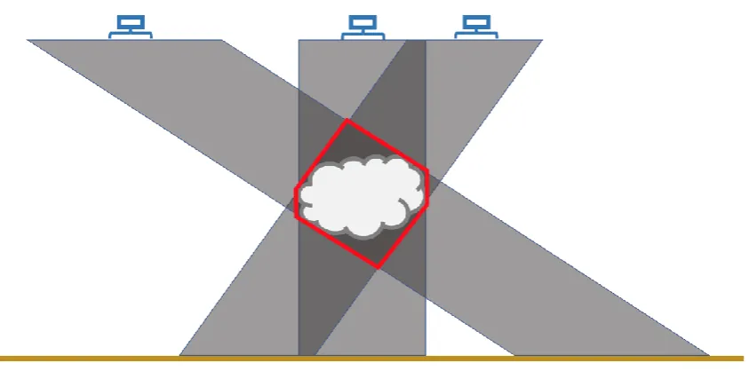
geo-registered locations of the cloudy pixels on the surface to the sensor‘s location according to the sensor‘s viewing zenith and azimuth angles, hence representing the radiance paths from the observed cloud to the satellite. Then, a series of calculations with the geometric properties of the voxels and the rays determine the space overlapped at all view angles, which is deemed to be the maximum space within the domain that the cloud occupies. Figure 1 gives a schematic diagram of this process.
Figure 1. The blue objects at the top represent the satellite sensor retrieving images at three different view
angles. The gray areas represent the potential locations of the cloud in the atmospheric domain at each view
angle. The brown line at the bottom represents the surface on which the retrieved data are geo-registered. The
red lines encircle the space intersected by the three views, hence determined to be the maximum possible
space occupied by the cloud.
ground-based observations of cloud base height. However, we do not include the application of the cloud base height here, strictly focusing on the use of MISR data only.
This ray casting method presumes that any significant parcel of cloud in the atmosphere, unless occluded by another parcel, must be visible at all view angles. In other words, any parcel of cloud that does not appear in all view angles is considered either to be occluded or to have size and optical depth negligible for the purpose of volume
reconstruction. This assumption helps evade the pixels that are falsely determined cloudy in the cloud masks due to sun glint, which predominantly appears at only one or few MISR view angles [26].
3. Simulation with synthetic clouds
To understand and quantify the errors and uncertainties expected with the reconstruction method in the absence of truth when applied to MISR data, simulations were run with synthetically generated clouds. Synthetic satellite images were derived from these clouds through the process of image formation, and then were used as inputs in the cloud volume reconstruction simulations. The reconstructed volumes were then compared with the original ―synthetic-truth‖ clouds.
The image formation was conducted as follows. First, from a 3-D synthetic cloud field, a set of 2-D binary cloud masks were derived in a way that imitates MISR‘s retrievals with its nine along-track view angles of ±70.5°, ±60.0°, ±45.6°, ±26.1°, and 0° (nadir), the orbital height of 705 km, and the pixel resolution of 275 m. The ground instantaneous field of view (GIFOV) per pixel was set to be the square area occupied by the pixel, and the ground sampling interval (GSI) was set to be the same as the pixel resolution. The geo-registered locations of the pixels remained the same in all view angles, as in MISR data. The satellite camera location for each pixel was determined to imitate MISR‘s push-broom technique, such that it follows the change in the pixel location on the ground in the along-track axis but remains the same in the cross-track axis. This gave rise to the changes in view angle across the swath. The dimensions of the images were set such that they include the clear ends of the cloud. For the ray casting, the method of voxel boundary intersections was used: if the ray, cast from the geo-registered location of a pixel to the corresponding satellite camera location, passed through the boundary of any cloudy voxel, the pixel was determined cloudy. The voxel boundaries were determined in terms of geometric planes corresponding to the sides of the voxel cuboids, either perpendicular or parallel to the plane ground. This ray casting from all surface-registered pixels to all cameras produced synthetic perfect cloud mask images for each camera.
Reconstructions were run with the cloud masks gained from the image formation as inputs. Under the same geometric parameters as in the image formation, rays were cast from the geolocations of the cloudy pixels through the reconstruction domain to the corresponding satellite‘s locations, and every voxel whose boundary was intersected by a ray was
3.1. Cloud geometry
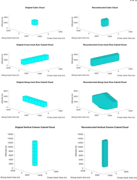
To examine the behavior of the reconstructions with respect to the observed cloud‘s shape, simulations were run on four types of geometrically simple synthetic clouds: cubic cloud, cross-track row cuboid cloud, along-track row cuboid cloud, and vertical column cuboid cloud. These basic cloud shapes were chosen to represent a unit parcel and the three fundamental axes (cross-track, along-track, and altitude) in three-dimensional geometry.
The synthetic clouds were put at the center of the observation‘s field of view during the image formation, so that the nadir line of sight from the satellite aligns with the center of the cloud volume. The cloud base height was set as 1650 m, within the usual altitude range (1-3 km) of real-world cumulus clouds. The cloud voxel resolution was set as 1650 m (i.e. the smallest unit volume of a reconstructed cloud was 16503 m3). This number was chosen to ensure that the cloud is larger than the pixel resolution of 275 m and evade the excessive overestimation of cloudiness by otherwise too tiny (sub-pixel) clouds in the image formation of perfect cloud masks [27]. The reconstruction voxel resolution was set as 275 m, same as the pixel resolution.
Figure 2. An example comparison between the original (left images) and the reconstructed (right images)
cloud volumes. From top to bottom: cubic cloud, cross-track row cuboid cloud, along-track row cuboid cloud,
and vertical column cuboid cloud. Here, the length of all the original cuboid clouds is 7 x 1650 = 11550 m.
The reconstruction voxel grid resolution is 275 m. All plots are in the same scale. MISR viewing geometry is
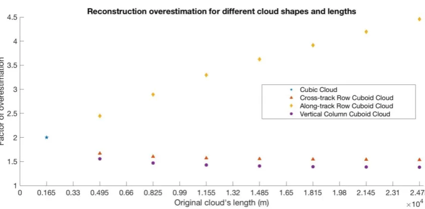
Figure 3. The results from different inputs of cloud shape and length. Here, the length is defined as the length
of the longest side of the cloud (as explained in Figure 2). The results are shown in factor of overestimation,
i.e. the reconstructed volume divided by the original volume. MISR viewing geometry is used. The original
cloud voxel resolution is 1650 m, and the reconstruction voxel resolution is 275 m.
As expected in our discussion of Figure 1, Figure 2 shows that in all cases the reconstruction yields an overestimation in the cloud volume. The overestimation is
particularly large in the case of the along-track row cuboid cloud, resulting from the greater building of prism at the cloud top and bottom. Figure 3 shows the factor of overestimation (the ratio of reconstructed cloud volume to the original cloud volume) as a function of the length of the longest side of the original cloud. The factor is around 2 for the cubic cloud, increases quite linearly at a rate of 0.1 km-1 as the cloud length increases in the along-track direction, and decreases asymptotically to around 1.5 or around 1.3 as the cloud length increases in the cross-track or the vertical direction, respectively (the numerical values are particular to this simulation case). In general, the less horizontally spread out in the along-track direction and the more vertically developed the cloud, the less the
overestimation in the cloud volume. Hence, this reconstruction method would yield the best results when applied to regions with vertically well-developed and horizontally narrow cumulus clouds, particularly if they are aligned in the cross-track direction. Note that it is intuitive to see that having more oblique views beyond the MISR view angles would lead to less of the prism building at the cloud top and bottom, thereby giving better reconstructions.
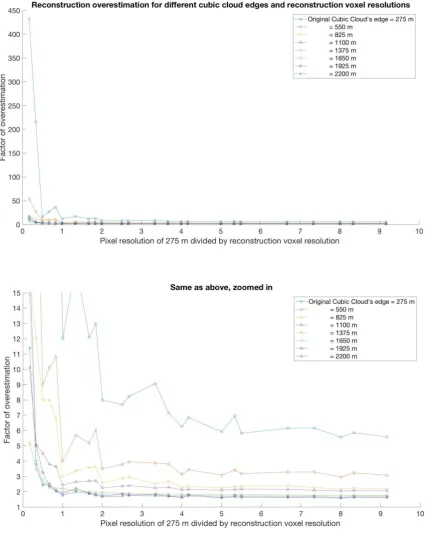
3.2. Image pixel resolution and reconstruction voxel resolution
results in terms of the factor of overestimation in cloud volume for cubic clouds with different sizes.
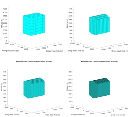
Figure 4. An example set of reconstructed cloud volumes for different reconstruction voxel resolutions. Here,
the original cubic cloud has an edge = 1650 m. The image pixel resolution of 275 m is used. All plots are in the
Figure 5. The factor of overestimation in cloud volume as a function of the ratio of image pixel resolution to the
reconstruction voxel resolution. Different plots indicate different sizes of the original cubic cloud.
2. For most of the cubic cloud sizes tested, overestimation is more or less stable when the reconstruction voxel resolution is smaller than or equal to the pixel resolution (i.e. when the ratio in x-axis of Figure 5 is 1). This is a useful reference for determining the reconstruction voxel resolution in the reconstructions from MISR data.
Figure 5 also shows that the greater the size of the original cloud with respect to the image pixel resolution, the smaller the overestimation of cloud volume. The relatively extensive overestimations at the smaller sizes of the original cloud (as shown especially by the cubic cloud with edge = 275 m) are due to the clear-conservative nature of the image formation, wherein smaller clouds still contribute the same to the cloudy determination of larger pixels (i.e. a pixel that is only partially cloudy is counted as fully cloudy) [27]. The overall bumpiness (lack of smoothness) in the curves is due to the mismatching of
resolutions, known as the resolution effect [27]. The 2-D resolution effect occurs between the original cloud and the synthetic satellite image pixels, and the 3-D resolution effect occurs between the synthetic images and the reconstruction voxels. In summary, we see that the reconstruction method would work best when the observed clouds are large and the reconstruction voxel resolution small in comparison to the pixel resolution.
4. Reconstruction from MISR data: methodology
The reconstruction from MISR entails details that are different from the conceptual simulations described in Section 3. In particular, 1) MISR data are geo-registered to a non-flat surface that accommodates the Earth‘s surface curvature; 2) cloud masks that classify cloudy and clear pixels may not be perfect; and 3) possible cloud movement due to wind and cloud morphing over the short time intervals between view angles call for the need for wind correction. These issues are addressed in the following subsections.
4.1. Reconstruction domain
The reconstruction domain of voxels is defined in a way that reflects the geometry behind the geo-registration of MISR data. MISR uses two map projections for its Level 1 and Level 2 products: ellipsoidal and terrain [28]. In this study, only the data in the ellipsoidal projection were used. The MISR ellipsoidal projection uses the World Geodetic System 1984 (WGS84) ellipsoid, with the equatorial radius of 6378137 m, the flattening factor of 298.257223563, and consequently the polar radius of 6356752 m [29]. The data is registered onto a
Figure 6. A diagram depicting the 2-D cross-section of a simplified reconstruction domain. Each voxel size
slightly increases as the altitude increases.
The ellipsoidal reconstruction is employed as opposed to the plane-ground
assumption used in Section 3, because the two could exhibit a significant difference in the reconstruction results. It was calculated, for the reconstruction voxel resolution = 1.1 km, that the ellipsoidal reconstruction domain, in comparison to the plane-ground reconstruction domain, could have a voxel grid distortion reaching around 10 m and the block grid distortion reaching around 870 m at the altitude of 20 km. Here, the voxel grid distortion is defined as the difference between the reconstruction voxel resolution (1.1 km) and the straight-line distance from a voxel center to another horizontally adjacent at the aforementioned altitude. The block grid distortion is defined as the difference between the MISR block‘s size in SOM Y (563.2 km) and the straight-line distance at the same altitude from one edge to another of the ellipsoidal reconstruction domain over the same block.
4.2. MISR science data
Multiple MISR science data products generated by the MISR science team and available on NASA‘s EOSDIS website were used in the reconstructions. Their names and version numbers are listed as follows:
MISR Radiometric Camera-by-camera Cloud Mask (RCCM) V004
MISR Level 1B2 Ellipsoid Data V003
MISR Ancillary Geographic Product (AGP) V001
MISR Geometric Parameters (GMP) V002
MISR Level 2 TOA/Cloud Height and Motion Parameters (TC_CLOUD) V001
The RCCM was one of the two input cloud masks used in the volume reconstruction. The algorithm and theoretical basis for the derivation of the RCCM can be found in the MISR Algorithm Theoretical Basis Document (ATBD) for Level 1 Cloud Detection [30], with the update for over ocean given by Zhao & Di Girolamo (2004) [26]. As its name suggested, the RCCM is derived independently for each of the nine MISR cameras. It has the pixel
low-confidence cloud, low-confidence clear, high-confidence clear, and no retrieval. In this study, the RCCM was converted to a binary cloud mask depending on the input choice of the classification levels. The RCCM pixels were assumed to have GIFOV and GSI equal to 1.1 km. Although in reality the GIFOV of the RCCM increases at oblique angles to as far as 1.53 km in the along-track direction, the effect of cloud overestimation by the oblique extension is negligible [26].
The L1B2 Ellipsoid radiance product provides the retrieved radiance values for MISR‘s red, green, blue, and near infrared spectral channels. The RGB images were used in selecting scenes appropriate for the reconstruction and the derivation of corresponding custom cloud masks at 275 m resolution, which were another input cloud mask to the volume reconstruction. The Ellipsoid Data also provides the reference time for each block at each view angle, which was used in the cloud mask wind correction (Section 4.4).
The AGP provides the geographical locations for each pixel at 1.1 km resolution, in terms of latitude and longitude. These values were used as the starting points of the cast rays during the reconstruction. The GMP provides the camera viewing zenith and azimuth values for each pixel at 1.1 km resolution. They were used to define the direction vectors of the cast rays.
The TC_CLOUD product provides cloud motion (speed) at 17.6 km resolution, in northward and eastward directions, and cloud top heights at 1.1 km resolution, both with and without wind correction [25]. All of the variables are reported at the reference time of the AN camera. The cloud motion variables were used to represent the wind field during the wind correction. The two variables for cloud top height were combined such that, given the heights with wind correction, all its no-retrieval pixels were replaced with the corresponding pixels from the heights without the wind correction which have less no-retrieval pixels. This was to minimize the number of no-retrieval pixels in the applied cloud top heights.
All of the products were interpolated as needed to match the pixel resolution of whichever of the two input cloud masks was used in the reconstruction. The details behind the interpolations can be found in [31].
4.3. Custom cloud mask
By design, the RCCM attempts to be clear-sky conservative, which at 1.1 km resolution leads to significant overestimation of cloud fractions, particularly for typical trade-wind cumulus clouds [32, 33]. As noted in Section 3.2, this could lead to significant overestimation of cloud volume, particularly for typical fair-weather cumulus sizes [34]. Therefore, a key concern rises from the onset, that the RCCM alone, with its 1.1 km resolution, may be too coarse for many cloud scenes of interest. Hence, to demonstrate improved reconstructions with a higher resolution than the operational RCCM, we produced a custom cloud mask at 275 m
resolution.
―whiter‖ in color than the background. It puts the threshold on the largest difference between each of RGB radiances and their mean. In other words, for each pixel with the RGB DNs
, , , and their average value
, it is determined cloudy if
(| | | | | |)
, where is the whiteness deviation
threshold value with . Here, the scale factors for converting the digital numbers to radiances have not been considered, assuming that they are consistent between different channels.
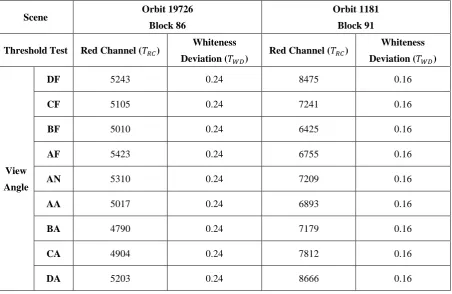
Table 1. Threshold values used for custom cloud masks for the selected scenes.
Scene Orbit 19726
Block 86
Orbit 1181
Block 91
Threshold Test Red Channel ( )
Whiteness
Deviation ( )
Red Channel ( )
Whiteness
Deviation ( )
View
Angle
DF 5243 0.24 8475 0.16
CF 5105 0.24 7241 0.16
BF 5010 0.24 6425 0.16
AF 5423 0.24 6755 0.16
AN 5310 0.24 7209 0.16
AA 5017 0.24 6893 0.16
BA 4790 0.24 7179 0.16
CA 4904 0.24 7812 0.16
DA 5203 0.24 8666 0.16
4.4. Wind correction
The reconstruction concerns an instant in time, so all input cloud masks need to be adjusted to the same time. However, the approximate 7-minute difference between the DF camera and the DA camera leads to possibly significant cloud motion and displacement by wind, as well as cloud morphing. Hence, there arises the need for wind correction to offset the cloud displacement and morphing between each view angle and the reference time of the reconstruction.
Since the cloud motion and height variables are all reported at the reference time of AN (the nadir view angle), and because the maximum time difference between view angles is minimized when AN is the reference time as opposed to others (less than 4 minutes), all wind corrections and therefore reconstructions in this study were conducted with reference to the time of AN of the block.
The wind correction poses a significant challenge. The reported cloud motion parameters only concern the cloud top boundary points observed for each pixel in the AN camera, so it is difficult to infer the overall wind field at different altitudes throughout the scene. That is, there is no direct information for the wind in other view angles, where the pixels of the same geolocations are looking through different portions of the atmosphere and different parts of the observed clouds. The reported wind at AN cannot simply be
if its index numbers, and , satisfy ( ) ( ) , where
(| | ) is the spreading addition number in pixel unit, | | the
selected wind vector with the block‘s highest speed, the time difference between an oblique camera and the AN, and the pixel resolution. This method operates on the assumption that the greatest wind reported is the actual greatest wind in the entire scene, in any 3-D direction, and throughout the time interval between different view angles. This is a reasonable assumption, since in reality 1) the wind is usually stronger in higher altitudes, and 2) the wind field does not change much in the span of several minutes.
The basic principle behind this cloud spreading method is that all pixels in non-nadir view angle images that are potentially cloudy at the time of the AN image are labeled as cloudy. This works because the nature of the reconstruction method tolerates the spreading of cloudy pixels. The reconstruction method assumes that the cloud should have been observed by all view angles and takes as cloudy only the voxels of the reconstruction domain that overlap as cloudy in all view angles. Hence, the cloudy pixels labeled by the spreading method can be simply considered as the candidates for the cloud‘s location at the time of AN.
This wind correction method adds another source of uncertainty that tends to
contribute a high bias to the reconstruction outcomes. The gross overestimation of the cloud is inevitably consequent, while the bias would depend on factors such as the true 3-D wind field and cloud movements. Therefore, the reconstruction results both with and without the wind correction are shown and compared in this study as a means of bounding the potential error caused by cloud motions over the time interval it takes MISR to observe the same scene.
4.5. Ray casting calculations
The final step in the reconstruction is the ray casting, where rays defined in terms of the MISR geometric and geographic parameters are cast through the pre-defined reconstruction domain, and voxels go through a series of calculations to be classified as clear or cloudy. The method of voxel boundary intersections is used.
Given the pre-determined reconstruction domain consisting of voxels on the WGS84 ellipsoid, the voxel boundaries are defined either as a plane of the form
or as an ellipsoid of the form
( ) ( )
, where A, B, C, and D are constants, H
voxel boundaries are calculated and recorded. Then, each intersection point is checked with respect to all other voxel boundaries in the reconstruction domain to see on which side of each of the voxel boundaries does it lie. This allows for pinpointing where the point lies in the reconstruction domain, in terms of its adjacent voxels. If any voxel in the entire domain has an intersection point in its boundary, then it is determined cloudy. The number of cast rays per pixel in one dimension (SOM X or SOM Y axis) is determined as
(
( )
) , where is the number of cast rays, the
horizontal voxel resolution, the vertical voxel resolution, and the maximum viewing zenith in the block. The addition of 2 at the end is to ensure that there are at least two cast rays per pixel in one dimension and therefore four in total, one at each corner of the pixel. This ensures that all voxels in the reconstruction domain fall the travel paths of all potential cast rays. Again, this process is repeated for all nine view angles, and only the voxels that have been determined cloudy by all nine angles are eventually classified as cloudy. For more discussion on this and other ray casting methods, see [31].
Afterward, the cloud top height (TC_CLOUD) is applied to reduce the
overestimation at the top of the reconstructed cloud (as mentioned in Section 2). This is done by casting rays from the AN cloud mask and calculating the intersection points only for the voxels as high as or below the cloud top height corresponding to the pixel from which the rays are cast. Only the voxels that remain cloudy under this constraint are kept to yield the final reconstructed cloud volume.
5. Reconstruction from MISR data: results
The results presented here come from scenes that are carefully hand-picked and show a good vertical development of clouds favorable for the multi-angle volume reconstruction from MISR data. Validation is difficult owning to the lack of truth for such clouds, therefore, we are guided by the validation on synthetic clouds in Section 3. Still, we did choose one scene where a basis for comparison was somewhat possible.
For each scene, a total of four types of results are shown as follows.
Input: RCCM. Wind correction: on.
Input: RCCM. Wind correction: off.
Input: custom cloud mask. Wind correction: on.
Input: custom cloud mask. Wind correction: off.
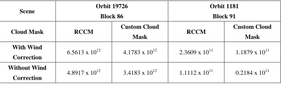
Table 2. Numerical results of the reconstructions. To simplify the volume calculations, each voxel was
assumed to be a rectangular cuboid. The entries are in cubic meters.
Scene Orbit 19726
Block 86
Orbit 1181
Block 91
Cloud Mask RCCM Custom Cloud
Mask RCCM
Custom Cloud
Mask
With Wind
Correction 6.5613 x 10
12
4.1783 x 10¹² 2.3609 x 10¹¹ 1.1879 x 10¹¹
Without Wind
Correction 4.8917 x 10
12 3.4183 x 10¹² 1.1112 x 10¹¹ 0.2184 x 10¹¹
5.1. Orbit 19726 Block 86
The reconstruction was run for the selected local region, shown in red boxes in Figure 7, in MISR Block 86 of Orbit 19726. It is over the Pacific Ocean far north of New Zealand near the Equator, observed on September 2, 2003, around 22:42:05 UTC. This scene was chosen for its cloud geometry favorable for reconstruction and to provide a cross-validation with the result from [21, 22].
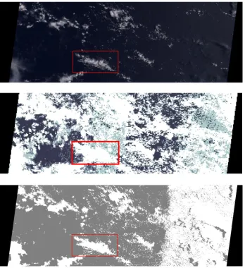
Figure 7 also shows the RCCM and the custom cloud mask at the AN camera. The thresholds in Table 1 were chosen specifically for the red box but applied here over the entire block. As a result, the effects of sun glint off to the right of the image are often misclassified as cloud, and the thinner clouds off to the left of the image are often classified as clear. In general, the RCCM produces greater cloud cover compared to the custom cloud mask, owing to its 1.1 km resolution versus the 275 m resolution of the custom cloud mask.
Figure 7. The RGB image, the RCCM, and the custom cloud mask of Orbit 19726 Block 86, at view angle AN.
In the RCCM, the white indicates the high confidence cloud, the light green the low confidence cloud, the gray
the low confidence clear, and the darker gray the high confidence clear. The black indicates no retrieval. The
region selected for the reconstruction is indicated in the red boxes. The widespread erroneous cloudiness on the
CF
BF
AF
AN
AA
BA
CA
DA
Figure 8. From left to right: the RGB image, the RCCM, the RCCM with the wind correction (cloud
Figure 9. The reconstruction results for four different cases at two different viewing perspectives. The units are
all in meters. The red box at the center is the overhead (nadir) RGB image of the reconstruction region, with
applied. Hence, the reconstructions with wind correction exhibit larger volumes than those without. In all cases, the wall of clouds stretching from the upper left to the lower right corner of the reconstruction region is seen, as expected in our mental constructions from the nine RGB images.
The reconstruction from the custom cloud mask without wind correction for this scene can be compared with the result from [21] which also did not include wind
correction, as shown in Figure 10. [21] used a stereo-photogrammertric method to retrieve both cloud-top heights and sides with a precision of about 200-300 m. In terms of the general shape, the reconstruction agrees with their result, showing the wall of clouds that stretch vertically up to around 8.5 km. The reconstruction shows greater horizontal width from around 2 to 5 km altitude, as [21]‘s result takes a concave shape. When the true cloud exhibits concavity in the along-track direction, our reconstruction method would be unable to detect it and create a convex volume with greater overestimation.
Figure 10. A cross-sectional comparison between the reconstructed volume from the custom cloud mask without the wind correction and the result from [21]. [21]‘s result consists of outcomes for eight stereo pairs of different view angles, but here they are all expressed in one color.
The second region selected for cloud reconstruction, shown in red boxes in Figure 11, is over the Atlantic Ocean south of West Africa, observed on March 8, 2000, around 11:33:19 UTC. This scene was chosen as it contains two vertically tall and horizontally narrow columns of clouds. As in the previous example, the thresholds (Table 1) were chosen specifically for the red box but applied here over the entire block. Figure 12 shows the ray casting domain around the selected reconstruction region, and Figure 13 shows the reconstruction results.
Figure 11. The RGB image, the RCCM, and the custom cloud mask of Orbit 19726 Block 86, at view angle
Figure 12. Same as Figure 8, but for the selected region in Orbit 1181 Block 91. The RGB images have been modified to increase the contrast between the ocean and the clouds for reader‘s view.
CF
BF
AF
AN
AA
BA
CA
This paper explored the 3-D cloud volume reconstruction from MISR using a ray casting method. First, simulations were done, with a handful of synthetically generated clouds and with respect to the observed cloud‘s geometry and the reconstruction resolution, to
understand and estimate the errors and uncertainties associated with the reconstruction method in various cases. Under the assumption of perfect cloud detection, it has been demonstrated that overestimation of cloud volume in the reconstruction would be smaller when the observed cloud is more developed in the vertical and cross-track directions and less developed in the along-track direction. In addition, overestimation would be smaller when the observed cloud‘s size is large and the reconstruction voxel resolution is small in comparison to the pixel resolution.
Then, reconstructions were done for the real MISR data using the 1.1 km resolution RCCM and the 275 m resolution custom cloud masks generated from MISR RGB radiance data. The Earth‘s surface curvature was reflected in the reconstruction domain and wind correction was performed by implementing the ―cloud spreading‖ method. Reconstruction results were shown for two hand-picked scenes, namely Orbit 19726 Block 86 and Orbit 1181 Block 91. The former case showed a good agreement with the result from [21]. Several tendencies were observed in both scenes. First, the RCCM results tend to
overestimate more than the custom cloud mask results. This is mainly because the greater ratio between the pixel resolution and the observed cloud‘s size leads to greater
overestimation of cloudiness in the cloud masks [32]. The greater precision (finer details) with the custom cloud mask results and the error evaluation with the synthetic clouds point to a need for MISR to move toward a cloud mask product with 275 m resolution for extensive production. Next, the results with the wind correction tend to overestimate more than the results without the wind correction, as anticipated in Section 4.4.
While we conclude that the reconstruction results are visually positive and agreeable to the human eye, and that the 3-D cloud volume reconstruction is possible with MISR using a ray casting method and proper cloud masks, several limitations need to be noted:
volumes. Another improvement could be a better validation of the reconstruction method by using 3-D radiative transfer simulations imitating MISR measurements applied to 3-D cloud fields generated from cloud resolving models. This could better reflect the nuances of cloud masking and cloud motion on cloud volume reconstruction (c.f., [38]).
Cloud masks with higher spatial resolutions are simply better for cloud volume reconstructions. Provided that the issue of computation is well handled, data from instruments with higher resolution could significantly improve the reconstruction results. Future work could make use of ASTER on board the same Terra satellite as MISR. ASTER looks at the same scene as MISR at the finer resolution of 15 m and with two view angles, and hence could help refine the reconstructed volumes and generate better results.
The application was limited to cases of vertically well-developed cumulus clouds that had been manually selected. The automation and operationalization of the
reconstruction program for all available MISR data remains a challenging task, which may be resolved when a technique for recognizing applicable scenes is developed, such as properly trained machine learning algorithms or artificial neural networks.
While the limitations are legitimate and require a significant future effort to be resolved, there are several practical implications that give reasons to move forward with the cloud volume reconstructions:
Provided that the reconstructions are verified with proper and enough validations, they could be used to study 3-D cloud distribution of a select geographical location for a climatological period of time, thanks to MISR‘s long-lasting operation of 18 years and counting and stable 10:30 am equator crossing time of its sun-synchronous orbit. Such studies cloud lead to understanding the clouds‘ impact on the local geography‘s radiation budget and further our understanding of the role of clouds in the Earth‘s radiation budget.
Once the reconstruction program is extensively used to generate and accumulate results for many different real-world cloud scenes, the collection of such data could be used to test the realism of the geometry of clouds produced in LES simulated models and cloud resolving models.
The reconstructions could be useful in providing the initial guess for future tomographic research involving MISR. Tomography is a potential tool in remote sensing retrievals of 3-D atmospheric profiles including cloud microphysical properties, and as explained in [36], the tomographic reconstructions could greatly benefit in accuracy and computations if the initial conditions such as cloud boundaries are specified.
overestimation of cloud area to the negligible amounts for real world clouds (e.g., [37]); to be able to estimate the cloud base height based on cloud shadow detection (e.g. [39]); and to provide improved precision in cloud stereoscopic height retrieval to the order of 10 m using a similar algorithm as in [25]. These recommendations would provide an excellent mission scenario for employing the ray casting reconstruction method for future cloud volume reconstructions.
7. Patents
Author Contributions: conceptualization, L. D. and B. L.; methodology, B. L. and L. D.; software, B. L.; validation, B. L.; formal analysis, B. L.; investigation, B. L., L. D., and G. Z.; data curation, B. L.; writing—original draft preparation, B. L.; writing—review and editing, B. L., G. Z., Y. Z., and L. D.; visualization, B. L.; supervision, G. Z., Y. Z., and L. D.; funding acquisition, L. D..
Funding: This research was funded by the National Aeronautics and Space Administration (NASA) through contract number NNX13AL96G, and by the Jet Propulsion Laboratory (JPL) through contract number 147871.
Acknowledgments: Special thanks to Dr. Céline Cornet for providing the data in [21, 22] for the comparison shown in Section 5.1.
Conflicts of Interest: The authors declare no conflict of interest.
References
1. Marshak, A., and A. Davis, 2005: 3D Radiative Transfer in Cloudy Atmospheres. Physics of Earth and Space Environments Series, Springer, Heidelberg, Germany. 2. Wallace, J., and P. Hobbs, 2006: Atmospheric Science: An Introductory Survey,
Second Edition. Academic Press, Oxford, UK.
3. Clothiaux, E. E., H. W. Barker, and A.V. Korolev, 2005: Observing Clouds and Their Optical Properties. In A. Marshak and A. Davis (Eds.), 3D Radiative Transfer in Cloudy Atmospheres (pp. 93-150). Springer, Heidelberg, Germany.
5. Ellingson, R. G., and E. E. Takara, 2005: Longwave Radiative Transfer in Inhomogeneous Cloud Layers. In A. Marshak and A. Davis (Eds.), 3D Radiative Transfer in Cloudy Atmospheres (pp. 487-519). Springer, Heidelberg, Germany.
6. Hinkelman, L. M., K. F. Evans, E. E. Clothiaux, T. P. Ackerman, and P. W. Stackhouse Jr., 2007: The effect of cumulus cloud field anisotropy on domain-averaged solar fluxes and atmospheric heating rates. J. Atmos. Sci., 64, 3499-3520.
7. Kobayashi, 1993: Effects due to cloud geometry on biases in the albedo derived from radiance measurements. J. Clim., 6, 120-128.
8. Várnai, T., and R. Davies, 1999: Effects of Cloud Heterogeneities on Shortwave Radiation: Comparison of Cloud-Top Variability and Internal Heterogeneity. J. Atmos. Sci., 56, 4206-4224.
9. Marshak, A., S. Platnick, T. Várnai, G. Wen, and R. F. Cahalan, 2006: Impact of 3D radiative effects on satellite retrievals of cloud droplet sizes. J. Geophys. Res. 111, DO9207, doi:10.1029/2005JD006686.
10.Zhang, Z., A. S. Ackerman, G. Feingold, S. Platnick, R. Pincus, and H. Xue, 2012: Effects of cloud horizontal inhomogeneity and drizzle on remote sensing of cloud droplet effective radius: Case studies based on large-eddy simulations. J. Geophys. Res.,
117, D19208, doi:10.1029/2012JD017655.
11.Di Girolamo, L., L. Liang, and S. Platnick, 2010: A global view of one-dimensional solar radiative transfer through oceanic water clouds. Geophys. Res. Lett., 37, L18809, doi:10.1029/2010GL044094.
12.Zhao, G., L. Di Girolamo, D. J. Diner, C. J. Bruegge, K. Mueller, and D. L. Wu, 2016: Regional changes in Earth‘s color and texture as observed from space over a 15-year period. IEEE Trans. Geosci. Remote Sens., 54(7), 4240-4249,
doi:10.1109/TGRS.2016.2538723.
13.Zinner, T., B. Mayer, and M. Schröder, 2006: Determination of three-dimensional cloud structures from high-resolution radiance data. J. Geophys. Res., 111, D08204,
doi:10.1029/2005JD006062.
14.Barker, H. W., M. P. Jerg, T. Wehr, S. Kato, D. P. Donovan, and R. J. Hogan, 2011: A 3D cloud-construction algorithm for the EarthCARE satellite mission. Q. J. R. Meteorol. Soc., 137, 1042-1058, doi:10.1002/qj.824
15.Ham, S.-H., S. Kato, H. W. Barker, F. G. Rose, and S. Sun-Mack, 2014: Effects of 3-D clouds on atmospheric transmission of solar radiation: Cloud type dependencies
inferred from A-train satellite data. J. Geophys. Res. Atmos., 119, 943–963, doi:10.1002/2013JD020683.
16.Ham, S.-H., S. Kato, H. W. Barker, F. G. Rose, and S. Sun-Mack, 2015: Improving the modelling of short-wave radiation through the use of a 3D scene construction
algorithm. Q. J. R. Meteo. Soc., 141, 1870-1883, doi: 10.1002/qj.2491
17.Fielding, M. D., J. C. Chiu, R. J. Hogan, and G. Feingold, 2014: A novel ensemble method for retrieving properties of warm cloud in 3-D using ground-based scanning radar and zenith radiances. J. Geophys. Res. Atmos., 119, 10912–10930,
20.Kassianov, E., T. Ackerman, R. Marchand, and M. Ovtchinnikov, 2003: Satellite multiangle cumulus geometry retrieval: Case study. J. Geophys. Res., 108, D3, 4117, doi:10.1029/2002JD002350, 2003.
21.Seiz, G., and R. Davies, 2006: Reconstruction of cloud geometry from multi-view satellite images. Remote Sens. Environ., 100, 143-149.
22.Cornet, C., and R. Davies, 2008: Use of MISR measurements to study the radiative transfer of an isolated convective cloud: Implications for cloud optical thickness retrieval. J. Geophys. Res., 113, D04202, doi:10.1029/2007JD008921.
23.Moroney, C., R. Davies, and J.-P. Muller, 2002: Operational Retrieval of Cloud-Top Heights Using MISR Data. IEEETransactions on Geoscience and Remote Sensing, Vol. 40, No. 7.
24.Muller, J.-P., A. Mandanayake, C. Moroney, R. Davies, D. J. Diner, and S. Paradise, 2002: MISR Stereoscopic Image Matchers: Techniques and Results. IEEETransactions on Geoscience and Remote Sensing, Vol. 40, No. 7.
25.Mueller, K., C. Moroney, V. Jovanovic, M. J. Garay, J.-P. Muller, L. Di Girolamo, and R. Davies, 2013: MISR Level 2 Cloud Product Algorithm Theoretical Basis. Jet
Propulsion Laboratory, California Institute of Technology. Retrieved July 3, 2017, from
https://eospso.gsfc.nasa.gov/atbd-category/45
26.Zhao, G., and L. Di Girolamo, 2004: A Cloud Fraction versus View Angle Technique for Automatic In-Scene Evaluation of the MISR Cloud Mask. Journal of Applied Meteorology, 43, 860-869.
27.Di Girolamo, L., and R. Davies, 1997: Cloud fraction errors caused by finite resolution measurements. Journal of Geophysical Research, 102, D2, 1739-1756.
28.Jovanovic, V. M., S. A. Lewicki, M. M. Smyth, J. Zong, and R. P. Korechoff, 1999: Level 1 Georectification and Registration Algorithm Theoretical Basis. Jet Propulsion Laboratory, California Institute of Technology. Retrieved June 14, 2017, from
https://eospso.gsfc.nasa.gov/atbd-category/45
29.National Geospatial-Intelligence Agency (NGA), 2014: Department of Defense World Geodetic System 1984, Its Definition and Relationships with Local Geodetic Systems. Retrieved June 25, 2017 from http://earth-info.nga.mil/GandG/publications/index.html 30.Diner, D. J., L. Di Girolamo, and E. E. Clothiaux, 1999: Level 1 Cloud Detection
Algorithm Theoretical Basis. Jet Propulsion Laboratory, California Institute of Technology. Retrieved June 28, 2017, from
31.Lee, B., 2017: Three-dimensional cloud volume reconstruction from the Multi-angle Imaging SpectroRadiometer (M.S. thesis). University of Illinois at Urbana-Champaign. Retrieved August 21, 2018, from http://hdl.handle.net/2142/99363.
32.Zhao, G., and L. Di Girolamo, 2006: Cloud fraction errors for trade wind cumuli from EOS-Terra instruments. Geophys. Res. Lett., 33, L20802, doi:10.1029/2006GL027088. 33.Jones, A. L., L. Di Girolamo, and G. Zhao, 2012: Reducing the resolution bias in cloud
fraction from satellite derived clear-conservative cloud masks. J. Geophys. Res., 117, D12201, doi:10.1029/2011JD017195.
34.Zhao, G., and L. Di Girolamo, 2007: Statistics on the macrophysical properties of trade wind cumuli over the tropical western Atlantic. J. Geophys. Res., 112, D10204,
doi:10.1029/2006JD007371
35.Wielicki, B. A., and L. Parker, 1992: On the determination of cloud cover from satellite sensors: The effect of sensor resolution. J. Geophys. Res., 97, 12799-12823.
36.Levis, A., Y. Y. Schechner, A. Aides, and A. B. Davis, 2015: Airborne Three-Dimensional Cloud Tomography. In Proc. IEEE ICCV, 3379-3387. 37.Dey, S., L. Di Girolamo, and G. Zhao, 2008: Scale effect on statistics of the
macrophysical properties of trade wind cumuli over the tropical western Atlantic during RICO. J. Geophys. Res., 113, D24214, doi:10.1029/2008JD010295.
38.Yang, Y., and L. Di Girolamo, 2008: Impacts of 3-D radiative transfer effects on satellite cloud detection and their consequences on cloud fraction and aerosol optical depth retrievals. J. Geophys. Res., 113, D04213, doi:10.1029/2007JD009095.