Protein-Protein Interaction Network Alignment

Scholarship@Western

Scholarship@Western

Electronic Thesis and Dissertation Repository

12-16-2014 12:00 AM

Protein-Protein Interaction Network Alignment

Protein-Protein Interaction Network Alignment

Yu Qian

The University of Western Ontario

Supervisor Dr. Lucian Ilie

The University of Western Ontario Graduate Program in Computer Science

A thesis submitted in partial fulfillment of the requirements for the degree in Master of Science © Yu Qian 2014

Follow this and additional works at: https://ir.lib.uwo.ca/etd

Part of the Computer Sciences Commons

Recommended Citation Recommended Citation

Qian, Yu, "Protein-Protein Interaction Network Alignment" (2014). Electronic Thesis and Dissertation Repository. 2579.

https://ir.lib.uwo.ca/etd/2579

This Dissertation/Thesis is brought to you for free and open access by Scholarship@Western. It has been accepted for inclusion in Electronic Thesis and Dissertation Repository by an authorized administrator of

(Thesis format: Monograph)

by

Yu Qian

Graduate Program in Computer Science

A thesis submitted in partial fulfillment

of the requirements for the degree of

Masters of Science

The School of Graduate and Postdoctoral Studies

The University of Western Ontario

London, Ontario, Canada

c

Proteins are some of the building blocks of organisms. They usually perform their func-tions by interacting with each other and forming protein complexes. A protein-protein interaction network is a graph that consists of proteins as vertices and their interactions as edges. Protein-protein interaction network alignment is very important in identifying protein complexes and predicting protein functions. Many algorithms based on graph theory have been developed to improve the accuracy of alignment, but due to the sparsity of protein-protein interactions, the result is far from satisfactory.

We propose to improve the network alignment through adding protein interactions to existing PPI networks. In order to assess the improvement, we devise four groups of experiments and compare their results. The quality of PPI network alignment is assessed through the number of known protein complexes that are discovered. Significant improvement is obtained, up to 70% additional complexes being discovered after adding interactions. Other consequences are observed as well. Out of the two programs we compare, AlignMCL and MaWISH, the former performs significantly better whereas the latter is more stable. Further, adding predicted PPIs is not as efficient as adding PPIs from existing databases. Finally, we show that smaller but more reliable sets of interactions perform better than larger PPI sets.

Keywords: protein-protein interaction, network alignment, PPI prediction

My deepest gratitude goes first and foremost to my supervisor, Dr. Lucian Ilie, for his careful guidance and rigorous attitude in research. I will never reach here without his help.

Second, I’d like to show my heartfelt appreciation to all my labmates for offering me advice and assistance which helped me a lot in the research, especially Yiwei Li, who provided me huge support in my experiments.

I also want to express my gratitude to my friends Linfang Jin and Yanjun Xu, their long-lasting encouragement and trusts make me self-confident and brave.

Last but not least, I wish to thank my beloved parents, without their unyeilding support and endless encouragement, Thank you for the faith in me.

Certificate of Examination ii

Abstract ii

List of Figures vi

List of Tables viii

1 Introduction 1

2 Background 3

2.1 Proteins and Interactions . . . 3

2.2 Protein-Protein Interaction Prediction . . . 4

2.3 Protein Orthologs . . . 6

2.4 Protein-Protein Interaction Network Alignment . . . 7

2.4.1 Global Network Alignment . . . 8

2.4.2 Local Network Alignment . . . 13

2.5 Existing PPI-related Databases . . . 16

3 Improving PPI Network Alignment 19 3.1 Our Proposed New Idea . . . 19

3.2 Software Used For Investigation . . . 19

3.2.1 PPI prediction . . . 19

3.2.2 PPI network alignment . . . 21

3.3 Data Preparation . . . 28

3.3.1 Datasets . . . 28

3.4 Experimental Setup . . . 31

3.4.1 PPI Prediction . . . 31

3.4.2 Network Alignment . . . 32

4 Results and Evaluation 34 4.1 Evaluation guidelines . . . 34

4.2 Test Datasets . . . 35

4.3 Results and analysis . . . 36

4.3.1 Improvement of PPI network alignment . . . 36

4.3.2 Performance comparison of AlignMCL and MaWISH . . . 39

4.3.3 Reliability of predicted PPIs . . . 42

4.3.4 Intersection dataset performance . . . 42

5 Conclusion and Further Research 48

Bibliography 50

Curriculum Vitae 57

2.1 Protein Complex. (From: bioproximity.com) . . . 4

2.2 A Protein-Protein Interaction Network for yeast. (From: [39]) . . . 5

2.3 Overlap of PPIs between high-throughput traditional experiments. (From: [18]) . . . 5

2.4 Gene homologs. (From: bioweb.uwlax.edu) . . . 7

2.5 An example of score calculation in the IsoRank Algorithm (From: [41]) . 9 2.6 2- to 5- Graphlets (From: [50]) . . . 12

2.7 Graphlet Degree Vector (From: [50]) . . . 12

2.8 Alignment Graph in PathBLAST (From: [19]) . . . 14

2.9 NetworkBLAST Framework (From: [45]) . . . 15

3.1 Steps for PIPE algorithm. (From: [38]) . . . 20

3.2 duplication/divergence Model. (From: ([26])) . . . 22

3.3 (a) An instance of local network alignment. The proteins that have nonzero similarity scores are shaded the same (b) A local alignment induced by the protein subset pair{u1, u2, u3, u4} and {v1, v2, v3}. (From: [26]) . . . 24

3.4 Alignment Graph of the example in Figure 3.3. (From: [26]) . . . 24

3.5 An Alignment Graph in AlignNemo. (From: [10]) . . . 26

3.6 MCL of 2-path weighted 1, cells in bold in each row indicates a cluster. (multiply the original matrix by itself once) (From: [12]) . . . 27

3.7 Inflation of the matrix in MCL, r is the inflation level, rescale means normalize all the columns (From: [12]) . . . 28

3.8 A protein sequence in FASTA format; the first line with “>” is description, then sequence follows. . . 29

4.1 AlignMCL vs MaWISH for fly. . . 40

4.2 AlignMCL vs MaWISH for yeast. . . 41

4.3 Martin’s vs I2D for fly. . . 43

4.4 Martin’s vs I2D for yeast. . . 44

4.5 DIP vs DIP&I2D for fly. . . 45

4.6 DIP vs DIP&I2D for yeast. . . 46

2.1 Network Alignment Algorithm Summary . . . 8 2.2 Global Network Alignment Algorithm Comparison (From: [17]) . . . 13 2.3 Local Network Alignment Algorithm Comparison. (One subnetwork (or

subgraph) found by an alignment algorithm is called a solution.) (From: [10]) . . . 16 2.4 PPIs data from DIP and I2D. (From: DIP and I2D web interface) . . . 18

3.1 PIPE run time analysis . . . 21 3.2 Protein Sequences of fly and yeast . . . 28 3.3 PPIs of fly and yeast. (DIP&I2D stands for the common interactions

shared by both DIP and I2D) . . . 29

4.1 Statistics of known protein complexes . . . 36 4.2 Results for adding Martin’s predicted interactions to DIP dataset. . . . 37 4.3 Results for adding I2D’s interactions to DIP dataset. . . 37 4.4 Results for adding Martin’s predicted interactions to DIP&I2D dataset. 37 4.5 Results for adding I2D’s interactions to DIP&I2D dataset. . . 37 4.6 PPI network alignment improvement due to adding interactions. The

tables correspond in order to the data in Tables 4.2-4.5. . . 38

Introduction

It is well known that proteins in cells often interact with each other to perform various important functions. The protein-protein interaction (PPI) network of an organism is a graph representing these interactions as edges between proteins as vertices. The PPI network contains pathways, complexes and modules of crucial importance for the good functioning of the organism [18].

Our understanding of the PPI networks can be enhanced by network alignment. A significant amount of work has been done to reveal protein functions through analysis of PPI networks. Global and local network alignment are the two main categories of network alignment. As distant species do not have large regions of global network similarity, local network alignment is of more value than global network alignment. Excellent algorithms, such as MaWISH [21] and AlignMCL [24] were proposed to tackle local network align-ment. MaWISH constructs the alignment graph according to a gene evolution model, while AlignMCL devised a novel approach to construct it through a new concept called

union graph. When searching subgraphs in the alignment graph, MaWISH reduces the problem to a maximum-weight subgraph problem, while AlignMCL uses a cluster finding program based on Markov random walks.

There is no golden rule to measure the performance of network alignment. The most popular way is to compare the protein overlaps between subgraphs and some known protein complexes. According to this rule, AlignMCL is currently the best one [24]. But still, it can only detects less than 50% known protein complexes.

Another fact about PPIs worth noting is that the number of known PPIs is very small, the actual number might be significantly higher. Therefore, predicting new reliable PPIs may help us to reveal more unknown protein functions. Experimental methods such as Y2H (Yeast two-hybrid) [18] are used in early PPI prediction, but they are both labor and time consuming and their false positive rates are high. Due to these limitations, many computational approaches like Martin’s [25] and PIPE [38] are proposed. Mar-tin’s program uses support vector machines (SVM) on signature products, while PIPE computes a prediction matrix based on sequence similarities between proteins.

According to the limitations of network alignment algorithms, we proposed a new idea for improving local network alignments by incorporating predicted PPIs. We investigate and select the best PPI prediction program to enrich existing PPI networks, then we perform local network alignment on these new PPI networks. The experimentals confirm our expectation: more protein complexes are detected after adding PPIs.

Background

This chapter introduces some basic concepts about proteins, protein-protein interactions (PPIs) and PPI prediction. Then, the two main categories of PPI network alignment are discussed, along with some popular PPI databases.

2.1

Proteins and Interactions

Proteins are key components of cellular machinery. They consist of twenty kinds of amino acids and fold into various 2D and 3D structures. They play multiple roles, including transferring signals, controlling the function of enzymes, and regulating production and activities in the cell [52].

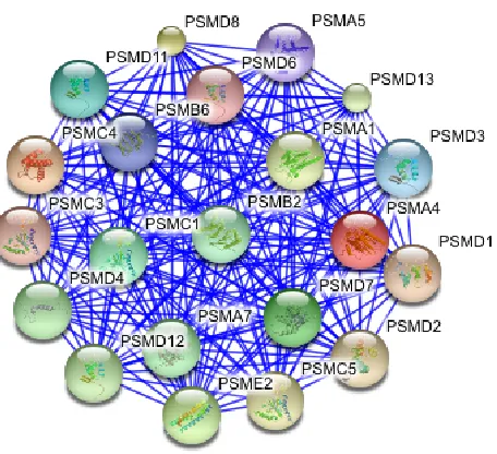
To achieve their key functions, proteins usually interact with each other. Some of the PPIs are permanent, while others are transient and happen only during certain cellular processes. Groups of proteins that interact together to perform a certain function are called protein complexes. Figure 2.1 shows an example of a protein complex in a cell. Protein pathways and modules are another two functional structures formed by proteins through PPIs. A PPI network consists of all the proteins in a species together with the interactions between proteins. Figure 2.2 shows a real PPI network constructed using 11,000 yeast interactions [18]. Protein complexes, pathways and modules are subgraphs of the PPI network. They are however not apparent from the network and need to be discovered.

PPIs are very important in molecular biology, as they help us to understand a protein’s function and behavior. They also help us to predict the biological processes that a protein of unknown function is involved in, so it is meaningful to find as many protein complexes in the PPI networks as possible.

Figure 2.1: Protein Complex. (From: bioproximity.com)

2.2

Protein-Protein Interaction Prediction

PPIs are critical to the integrity of PPI networks [5, 34, 43]. InSaccharomyces cerevisiae, there are early estimates of between 10,000 and 40,000 PPIs, out of a potential 19 million possible protein pairs, and the actual number might be significantly higher than these predictions.

Figure 2.2: A Protein-Protein Interaction Network for yeast. (From: [39])

low level of overlap between different experimental methods [18]. Figure 2.3 shows the overlap of PPIs between traditional experiments.

More accurate methods to predict PPIs are computational techniques, which can be classified into six general categories: methods based on genomic information, evolution-ary relationships, three-dimensional (3D) protein structure, protein domains, network analysis and primary protein structure [34]. Numerous methods have been developed to predict PPIs that take advantage of the sequence, structure or the genomic context of the query proteins [18]. Two leading programs are Martin’s [25] and PIPE (Protein-Protein Interaction Prediction Engine) [38].

2.3

Protein Orthologs

With the rapidly growing amount of sequence data, many scientists are asking which genes one species has in common with other species. A particularly important question is which genes in one species are sharing the exact same biological function with genes in simpler organisms. To be able to infer which genes have the same function, we need to understand how the genes evolved.

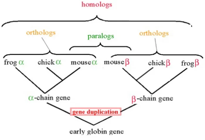
In biology, two genes related by descent from a common ancestral DNA sequence are called homologs. More specifically, if two genes are separated by the event of speciation, we call them orthologs; otherwise, if they are separated by the event of genetic duplica-tion, we call them paralogs. Figure 2.4 is an example of the formation of orthologs and paralogs. Orthologs retain the same function in the course of evolution, whereas paralogs evolve new functions, even if these are related to the original one.

Figure 2.4: Gene homologs. (From: bioweb.uwlax.edu)

Current approaches of orthology assignment can be classified into: (1) graph-based methods, such as InParanoid [20], eggNOG [29], OrthoMCL [22] and (2) tree-based methods, such as Ensembl Compara [2].

2.4

Protein-Protein Interaction Network Alignment

PPI networks are commonly represented as graphs, with nodes corresponding to proteins and edges representing PPIs. Most of the PPI networks are undirected and represent only binary interactions. An alignment is a mapping between these graphs. Network alignment, in its general form, is a computationally hard problem, since it can be related to the subgraph-isomorphism problem, which is known to be NP-complete. Effective techniques for solving this problem rely on suitable formulations of the alignment prob-lem, use of heuristics to solve these problems, or the use of alternate data to guide the alignment process [44].

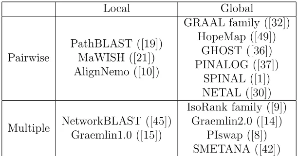
At a high level, the network alignment problem can be classified as global alignment

summary of current popular network alignment programs. Local Global Pairwise PathBLAST ([19]) MaWISH ([21]) AlignNemo ([10])

GRAAL family ([32]) HopeMap ([49])

GHOST ([36]) PINALOG ([37])

SPINAL ([1]) NETAL ([30])

Multiple NetworkBLAST ([45]) Graemlin1.0 ([15])

IsoRank family ([9]) Graemlin2.0 ([14])

PIswap ([8]) SMETANA ([42]) Table 2.1: Network Alignment Algorithm Summary

2.4.1

Global Network Alignment

Given a set of networks G = {G1, G2, ..., Gk}, a global network alignment requires all

nodes in all networks to be aligned. To achieve this goal, biological information from protein sequence similarity and topological information from a PPI network are used. Many algorithms make full use of this information to conduct global network alignment. The global network alignment is used to establish functional orthologs across species.

The two main steps in global network alignment are: 1) Compute node similarity between proteins from each input network and represent it as a matrix, 2) Extract node mapping from the matrix where seed and extension, bipartite matching or other heuristic strategy can be used. The IsoRank family [9] and the GRAAL family [32] are two traditional examples.

IsoRank

IsoRank is the first method to compute global alignment between the S.cerevisiae and

D.melanogaster PPI networks. The idea is: a nodeiinG1 is mapped to a nodej inG2 if

uses a similar idea as Google’s PageRank technique [33]. Also it was formalized as an eigenvalue problem.

IsoRank uses the following formula to calculate the similarity score Rij of protein i

and protein j:

Rij =

X

u∈N(i) X

v∈N(j)

1

|N(u)||N(v)|Ruv i∈V1, j ∈V2 (2.1)

where V1 and V2 are the sets of nodes in network G1 and G2 and N(a) is the set of

neighbors of node a. The value of Rij depends on the score of neighbors of i and j,

which, in turn, depend on the neighbors of the neighbors and so on. An example is shown in Figure 2.5.

Figure 2.5: An example of score calculation in the IsoRank Algorithm (From: [41])

We can incorparate biological information to this model through assigning weights to the graph; the above equation becomes:

Rij =

X

u∈N(i) X

v∈N(j)

w(i, u)w(j, v)

P

r∈N(u) P

q∈N(v)w(q, v)

Ruv i∈V1, j ∈V2 (2.2)

This equation can be further rewritten into a matrix form:

R=AR (2.3)

where

A[i, j][u, v] =

     1

|N(u)||N(v)| if (i,u)∈E1 and (j,v)∈E2

0 otherwise

(2.4)

A is a |V1||V2| ∗ |V1||V2| matrix and A[i, j][u, v] refers to the entry at the row (i, j) and

column (u, v).

It is clear that this is an eigenvalue problem, where R is the principal eigenvalue of

A. Then, maximum-weight bipartite matching is used to find the best matching for this graph. A greedy algorithm can be used here: identify the highest score Rpq and output

the pairing (p, q); then, remove all scores involving p or q; repeat this process until the list is empty.

IsoRankN [9] extends the same idea to aligning multiple networks.

GRAAL family

GRAAL [32] proposed an algorithm with the cost function based solely and explicitly on a strong, theoretically grounded and direct measure of network topological similarity. This method is flexible to incorporate biological data if we are trying to understand complex biological phenomena.

GRAAL first computes a matrix C of costs of aligning each node in G1 with each

node in G2. The rows of C correspond to nodes in G1 and the columns correspond to

nodes inG2. When computing the cost of aligning a node ufromG1 with a node v from

G2, GRAAL takes into account their signature similarity as well as their degrees. The

cost of aligning nodes u and v is computed as:

C(u, v) = 2−((1−α)∗ deg(u) +deg(v)

maxdeg(G1) +maxdeg(G2)

A cost of 0 corresponds to a pair of topologically identical nodesv andu. The advantage of GRAAL lies in computing the similarity score S(u, v) using graphlet degree signature and signature similarity [50]. Graphlets are small connected non-isomorphic induced subgraphs of a large network. Signature similarity counts the number of edges that a node touches in each graphlet; these numbers consist of the vector of graphlet degrees. We can understand the similarity simply as the number of shapes a node is part of.

In a general graph, two nodes can only form one shape; the 2-node graphlet is shown in Figure 2.6, while 3 nodes can form two non-isomorphic shapes. In each shape, nodes in the symmetric positions are called isomorphic. According to the same rule, 4 nodes have 6 graphlets, while 5 nodes can have at most 21 graphlets. Given these 29 graphlets in total, we then count how many non-isomorphic nodes are there in each graphlet. The two nodes in the 2-node graphlet are isomorphic, so we just count them once, and we call them an orbit, In the 2 3-node graphlets, we find 3 orbits. There are 73 orbits in total in all 2-node to 5-node graphlets.

Figure 2.7 is an example of graphlet degree vector, for the graph in the figure; node

v appears in 5 different 2-node graphlets, so GDV(0) = 5. v also appears as end node in two 3-node graphlets, so GDV(1) = 2. The Graphlet Degree Vector is computed this way.

Spheres are then built after the similarity matrix C is computed. A sphere of radius

r around a node u in a network G is the set of nodes SG(u, r) = {v ∈ G : d(u, v) = r}

that are at distance r from node u. d(u, v) is the length of the shortest path from u to

v. The node pair (u, v) with lowest score in C is selected as initial seed. The sphere of

uand the sphere of v are constructed inG1 and G2, respectively. Spheres with the same

radius are then aligned greedily and the algorithm stops when all the nodes in one input network are aligned to nodes in the other network.

Figure 2.6: 2- to 5- Graphlets (From: [50])

Figure 2.7: Graphlet Degree Vector (From: [50])

Other Algorithms

GEDEVO outperforms SPINAL and GRAAL in computing edge correctness [17]. Although many algorithms have been designed to tackle the global network alignment problem, the result is far from perfect due to the biological characteristics of the PPI networks. Another difficulty is that there is no golden rule to measure the performance of network alignment. For global network alignment, some often used parameters are edge correctness, node correctness, interaction correctness [30] and so on. Edge correctness is the percentage of edges (interactions) of the first network that are aligned to edges in the second network, while interaction correctness is the percentage of interactions of the first network that are aligned with correct interactions in the second alignment. Table 2.2 gives a comparison between some state-of-the-art global network alignment algorithms for a variety of networks; see [17] for more details. Note that none of them can reach a correctness rate greater than 50%.

Network 1 Network 2 Edge Correctness(%)

GEDEVO MI-GRAAL C-GRAAL SPINAL

Campylobacter jejuni Escherichia coli 33.70 24.60 22.56 22.09

Mesorhizobium loti Synechocystis sp.(PCC6803) 43.60 39.88 33.19 25.86

Saccharomyces cerevisiae Homo Sapiens 38.14 21.38 22.20 19.33

Homo Sapiens Saccharomyces cerevisiae 30.40 26.15 24.15 25.59

Saccharomyces cerevisiae Drosophila Melanogaster 20.79 17.73 20.59 21.07

Drosophila Melanogaster Homo Sapiens 21.88 - 27.36 27.04

Homo Sapiens Homo Sapiens 89.37 - 47.07

-Table 2.2: Global Network Alignment Algorithm Comparison (From: [17])

2.4.2

Local Network Alignment

Global network alignment attempts to capture a global picture of the whole input net-works. Distant species do not have large regions of global network similarity and it is more appropriate to search for local similarities. Local network alignment corresponds to a relationship defined over a subset of vertices in the input network, which is used to extract many conserved substructures (modules, pathways and complexes) from a set of species. A number of algorithms have been proposed for local network alignment.

each node denotes a pair of protein orthologsaanda0, and each edge denotes a conserved protein interaction, that is, an interaction observed for both (a, b) and (a0, b0). Sometimes, in order to tolerate a certain amount of missing interaction data, “indirect” edges are also defined if a pair of proteins interacts in one species (e.g. a and b interact) and the other pair of proteins (e.g. a0 and b0) is at distance at most two in their corresponding networks [47]. 2) Extract dense subgraphs from the alignment graph.

PathBLAST [19] and NetworkBLAST [45] are two early attempts for local network alignment. Protein sequence similarity is used to merge nodes from input networks. In PathBLAST and NetworkBLAST, a cut-off BLAST E-value (e.g., 10−7_{) is used to}

define the protein sequence similarity of two proteins. PathBLAST then defines match,

mismatchandgapas in sequence alignment to represent the alignment graph (see Figure 2.8). After the alignment graph is built, PathBLAST extracts high-scoring pathways. It generates a sufficient numbers of acyclic subgraphs and then uses dynamic programming to compute highest-scoring pathways.

PathBLAST was improved to a more efficient program called NetworkBLAST ([45]). The construction of the alignment graph in NetworkBLAST is more clear and flexible as proteins at distance 2 are assumed to interact, while in PathBLAST, gaps and mismatches are not allowed to occur consecutively. Subnetwork search over the alignment graph is defined to find high-scoring subnetworks based on a probabilistic model. The probabilistic model includes a real model in which every interaction should be present with high probability, and a random model, where the probability of an interaction depends on the total connections in the network. Then the log likelihood ratio defined on the two models are the score of the subnetwork over the subset of vertices U. Figure 2.9 shows the framework of NetworkBLAST used in local multiple network alignment.

Figure 2.9: NetworkBLAST Framework (From: [45])

According to the model above, the local network alignment problem can be reduced to finding heavy subgraphs heuristicaly in the alignment graph. NetworkBLAST first computes seeds with highest score at size 3, and adds a node which will increase the score to the seed iteratively. The size of subgraphs is limited to 15 nodes. For each node, it outputs the 4 highest-scoring subgraphs as the final result.

A novel algorithm, MaWISH, is based on duplication/divergence model with focus on understanding the evolution of PPI networks ([26]). AlignNemo improved local network alignment in two ways: 1). Adopted the newest protein orthologs information collected by Inparanoid algorithm [20], 2). The score assigned to each edge is based on an efficient construction of the alignment graph which incorporates topological information present in the original networks in terms of number, reliability and significance of paths of length less than or equal to 2 between two nodes [10].

AlignNemo and MaWISH are currently the leading programs for local network align-ment, which also find many known complexes. Table 2.3 shows some comparison of Networkblast, MaWISH and AlignNemo. In this comparison, the test datasets include 22,969 interactions in fly (Drosophila melanogaster), 22,254 interactions in yeast ( Sac-charomyces cerevisiae) and 78,559 weighted interactions in human (Homo sapien), more details are described in [10]. But due to the sparsity of protein interactions, many com-plexes remain undiscovered. AlignNemo was improved by adopting a new clustering algorithm; the new software is named AlignMCL [28].

The challenge in network alignment is not merely in designing an excellent algorithm to find more complexes. Overcoming the limitation of lacking protein-protein interactions is of the same importance, and a lot of work remains to be done in this area.

Algorithms fly-yeast fly-human

Solution size Complexes Founded Solution size Complexes Founded

NetworkBLAST 329 30 45 13

MaWISH 175 29 87 60

AlignNemo 242 52 115 87

Table 2.3: Local Network Alignment Algorithm Comparison. (One subnetwork (or sub-graph) found by an alignment algorithm is called a solution.) (From: [10])

2.5

Existing PPI-related Databases

in order to provide complete interactomes. The first of these databases was the Database of Interacting Proteins (DIP). Since that time, the number of public databases has been increasing. Databases can be subdivided into primary databases, meta-databases, and prediction databases [11].

• Primary databases collect information about published PPIs proven to exist via small-scale or large-scale experimental methods. Examples: DIP, I2D, Hint, DroID, BIND, BioGRID, HPRD, IntAct Molecular Interaction Database, MINT, MIPS-MPact, and MIPS-MPPI [11].

DIP (Database of Interaction Proteins) combines information from a variety of sources to create a single, consistent set of PPIs. The data stored in DIP has been curated, both manually, by expert curators, and automatically, using computational approaches that utilize knowledge about the PPI networks extracted from the most reliable, core subset of DIP data. In addition to the interaction information, DIP includes additional data regarding the proteins participating in PPI networks. This database is available at http://dip.doe-mbi.ucla.edu/. DIP is an early database from PPIs, and the number of PPIs in it is small when compared to other new databases.

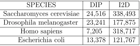
I2D (Interologous Interaction Database) is an on-line database of known and pre-dicted mammalian and eukaryotic PPIs. It has been built by mapping high-throughput data between species. Thus, until experimentally verified, these in-teractions should be considered “predictions”. I2D remains one of the most com-prehensive sources of known and predicted eukaryotic PPIs. I2D is available at http://ophid.utoronto.ca/ophidv2.204/. Table 2.4 shows some statistics of PPIs.

• Meta-databasesnormally result from the integration of primary databases infor-mation, but also collect some original data. Example: Agile Protein Interaction Data Analyzer (APID), The Microbial Protein Interaction Database (MPID8), and Protein Interaction Network Analysis (PINA) platform.

Protein-Protein Interaction Prediction Database (PIPs), On-line Predicted Human Interac-tion Database, Known and Predicted Protein-Protein InteracInterac-tions (STRING), and Unified Human Interactome (UniHI).

SPECIES DIP I2D

Saccharomyces cerevisiae 24,516 338,493 Drosophila melanogaster 23,241 177,875 Homo sapiens 7,205 318,717 Escherichia coli 13,378 121,767

Table 2.4: PPIs data from DIP and I2D. (From: DIP and I2D web interface)

The most important information in the PPI databases that we need is the interacting proteins and their reliability scores.

Besides PPIs databases, some related databases about protein complexes, pathways and modules are also very important in PPI network alignment. These databases are not only important in protein functions research, they are also a vital standard to measure network alignment algorithms. CORUM (Comprehensive Resource of Mammalian pro-tein complexes) provides a resource of manually annotated propro-tein complexes from mam-malian organisms. All information is obtained from individual experiments published in scientific articles. Data from high-throughput experiments is excluded [4]. DPiM has 556 protein complexes for Drosophila, it defines potential novel members for several impor-tant protein complexes and assigns functional links to 586 protein-coding genes lacking previous experimental annotation [16]. DPiM is a large protein complex database and provides a valuable resource for analysis of protein complex evolution. CYC2008 is a comprehensive catalogue of 408 manually curated yeast protein complexes [46]. These gold standard datasets on protein complexes are key to inferring and validating PPIs.

Improving PPI Network Alignment

Designing a new alignment algorithm is not the only way to improve local network alignment. The result can be improved if many reliable PPIs are provided. We propose a new idea for improving network alignment through the combination of PPIs prediction and existing local network alignment algorithms.

3.1

Our Proposed New Idea

Our idea works as follows:

• Test existing PPI prediction algorithms and select the best one.

• Add high-scoring interactions to existing PPI networks.

• Perform network alignment on the new PPI networks.

• Verify the quality of the alignments obtained.

3.2

Software Used For Investigation

3.2.1

PPI prediction

According to the study of Park, Martin’s program [25] and PIPE [38] are the best two candidates for PPIs prediction [35]. PIPE can successfully predict new interactions based

on re-occurring short sub-sequences in an existing interaction database. Its major work-ing steps are shown in Figure 3.1. Given a protein sequenceAof lengthN, it checks every sliding window of sizewstarting from position 0 to positionN−w; the neighbors of the protein in the network which have the same window are added to the neighbors’ list of the query protein. When the neighbors’ lists of all the query windows are constructed, it searches all sliding windows of the same lengthw in another protein sequenceB, then compares the window with all the protein sequences in the neighbors’ list and records every hit into the matrixM. If the maximum score in the final matrix is greater than a given threshold, then proteinA and protein B are predicted to interact.

Figure 3.1: Steps for PIPE algorithm. (From: [38])

Table 3.1: PIPE run time analysis

PIPE version Time (one pair) Total(estimated) original PIPE 115 minutes 9,623 years window cached PIPE 4 minutes 334 years

Martin’s program uses signature products [25]. In this method, an amino acid se-quence is represented as a signature, which is a combination of three letters. For example, for the amino acid sequenceLV M T T M, the trimers are: LV M,V M T,M T T andT T M. They are made of a root (middle letter) and two neighbors (side letters). Then the sig-natures of those trimers are V (LM), M (VT), T (MT), T (MT), respectively. By adding those vectors together, the signature of the sequence isV(LM) +M(V T) + 2T(M T) [25]. Note that 2T(M T) comes from T(M T) +T(T M). To define the signature for protein-protein pairs, it uses the tensor product between vectors. In order to use support vector machines (SVM) in PPI prediction, the signature kernel is defined as the dot product of two signatures of two proteins. Then using machine learning methods, predictions will be made. In order to improve the performance, Martin adopted some adjustments, for example, it enforces symmetry in the protein-protein order to improve the signature product, then it normalizes the signature product to compensate for potential differences in the length of the amino acid sequences. More details are described in [25].

Martin’s program is faster than PIPE and the code is freely available, so we select Martin’s program for PPIs prediction.

3.2.2

PPI network alignment

According to the most popular evaluation method and the comparison we introduced in Chapter 2, MaWISH and AlignMCL are selected in our investigation.

MaWISH

network-specific parameter [6]. A network-growth model based on preferential attach-ment is proposed to generate networks with degree distribution similar to PPI networks. Duplication/divergence model is such a model of evolution that explains preferential attachment and power-law nature of PPI networks.

Figure 3.2 shows an example of protein duplication. Protein u1

0

is duplicated from proteinu1, andu1 loses its interaction withu3(dotted line), while, an interaction between

u1 and u1

0

is added to the network (dashed line). According to this model, MaWISH defines the local network alignment as a set of matches, mismatches (insertion or deletion) and duplications. For PPI networks G(U, E) and H(V, F), a protein subset pair P = ( ˜U ,V˜) is defined as a pair of protein subsets ˜U ⊆U and ˜V ⊆V. Any protein subset pair

P induces a local alignment A(G, H, S, P) = (M, N, D) ofG and H with respect to S, a similarity function between each pair of proteins in U ∪V:

• M - set of matches: Each match m∈M is associated with a score µ(m) to reflect the confidence of protein orthologs.

• N - set of mismatches: Each mismatch n ∈ N is associated with a score v(n) to penalize an insertion or deletion.

• D - set of duplications: Each duplication d ∈ D is associated with a score δ(d) to reflect duplications in one species.

Figure 3.2: duplication/divergence Model. (From: ([26]))

The total score of a local alignment based on the above scoring system is:

σ(A) = X

m∈M

µ(m) + X

n∈N

v(n) +X

d∈D

Every score in the formula is related to a similarity function S. The similarity score

S(u, v) quantifies the likelihood that protein u and v are orthologous. Equation 3.2 calculates the similarity score; in this equation, the COG database is used as a reference [48]. Let O be the set of all orthologous protein pairs derived from COG. Then O(uv) represents the event thatu andv are orthologous. ˜E is the threshold of BLAST E-value, MaWISH assumes the probability of a protein pair being orthologous is a monotonically decreasing function of the E-value. For example, for 100 orthologs in COG, if 30 orthologs among them have E-value smaller than ˜E and given a protein pair whose E-value is ˜E, then the probability of this protein pair to be ortholog is 0.3. COG can be substituted by any other ortholog database.

S(u, v) =P(E(u, v)<E˜|Ouv) =

{u0v0 ∈O :E(u0, v0)<E˜}

|O| (3.2)

Given this function, we define the score of match, mismatch and duplication as follows:

µ(uu0, vv0) =µS(uu0, vv0) (3.3)

v(uu0, vv0) =−vS(uu0, vv0) (3.4)

δ(uu0, vv0) =δ(S(u, u0)−d) (3.5)

δ, v andδ are all coefficients to tune the relative weight of corresponding events. S(u, u0) is the similarity score of protein uand protein u0.

Figure 3.3 is an example of the pairwise local alignment problem. The alignment graph is constructed according to the model above (Figure 3.4). Weights are assigned to the edges, which differs from NetworkBLAST who assign the protein ortholog information to nodes only. Then the local network alignment can be reduced to a maximum-weight subgraph problem. This problem is NP-complete.

Figure 3.3: (a) An instance of local network alignment. The proteins that have nonzero similarity scores are shaded the same (b) A local alignment induced by the protein subset pair {u1, u2, u3, u4} and {v1, v2, v3}. (From: [26])

while it is only loosely connected to the rest of the network. MaWISH adopted a greedy heuristic strategy for this problem because proteins that belong to a conserved module will induce heavy subgraphs, while being loosely connected to other parts of the graph. It works for maximum-weight subgraphs. After finding one subgraph, all aligned nodes are marked, then the process is repeated on unmarked nodes until no more subgraphs with positive weight can be found. The time complexity of MaWISH is O(|V||E|).

AlignMCL

The existing definitions of the alignment graph differ in the way of edge setting between two nodes. AlignMCL uses the same alignment graph construction method as Align-Nemo, but it is more efficient in subgraphs mining [10].

Given G1, G2 and a set of protein orthologs H = (u, v), u∈V1, v ∈V2 between the

nodes ofG1, G2, a union graph is defined on two kinds of nodes: (i) composite nodes

representing pairs of protein orthologs and (ii) simple nodes that don’t have homologs in the other network. Any edge contained in one of the input networks is represented in the union graph. An alignment graph in AlignNemo is a reduced version of the union graph in which only composite nodes are retained and an edge connects two nodes if there is at least one path of length less than or equal to 2 between the two nodes in the union graph; see Figure 3.5 for example.

An efficient edge scoring strategy based on union graph makes AlignNemo prevail over other methods. To score edges of two proteins (composite nodes), direct path and

indirect path at most distance 2 are treated separately (See Equation 3.6, 3.7, 3.8).

S1(a, b) =

w(E1(a)∩E1(b))

w(E1(a)∪E1(b))

(3.6)

S2(a, b) =

w(E2(a)∩E2(b))

w(E2(a)∪E2(b))

(3.7)

We use ELI to stands for the score of edges,ELI(a, b) is the score of the edge (a, b).

Sk(a, b) is the score of all paths at distance k betweena and b. Ek(a) is the set of paths

connecting a to its neighbors at distance k and w(Ek(a)) is the sum score of all paths

connectinga to its neighbors at distancek. MaWISH also allows for gaps or mismatches to connect conserved proteins at distance 2 in the aligned graph, but it is not able to account for the reliability of direct and indirect paths. Figure 3.5 is an example of alignment graph in AlignNemo and AlignMCL.

Figure 3.5: An Alignment Graph in AlignNemo. (From: [10])

Finding enough reliable subgraphs is always at the heart of the local network align-ment problem. It can be reduced to a clustering problem. The MCL (Markov CLustering) algorithm [12] is an excellent solution to extract clusters in a graph, but has never been used in PPI networks before. It is first adopted by AlignMCL in local network alignment to improve AlignNemo [24, 28].

that visits a dense cluster will likely not leave the cluster until most of the vertices in the cluster have been visited. MCL simulates a stochastic flow on the network that resembles a set of random walks on the graph. It means that a random walk is expected to cover a dense subgraph in an alignment graph.

There are two steps in MCL:

• Expand For each node in the graph, a stochastic flow spreading out from the node towards all the other nodes. This step is performed by repeatedly multiplying the normalized adjacency matrix of the graph by itself (See Figure 3.6). Nodes connected by multiple (and shorter) paths will be the endpoints of stronger flows.

• Inflation This step aims at enhancing flows within clusters and weakening inter-cluster flows. Inflation is simply squaring the matrix (see Figure 3.7) by r (the inflation level). It is important to tune an inflation level as it controls the extent of this strengthening/weakening. After inflation, the matrix is normalized on each column.

Figure 3.6: MCL of 2-path weighted 1, cells in bold in each row indicates a cluster. (multiply the original matrix by itself once) (From: [12])

Figure 3.7: Inflation of the matrix in MCL,ris the inflation level, rescale means normalize all the columns (From: [12])

3.3

Data Preparation

Due to the variety of different protein sequences and PPI databases used in different steps, a significant amount of data preparation has to be performed before any experiments.

3.3.1

Datasets

We will use the dataset offly (Drosophila melanogaster) and yeast (Saccharomyces cere-visiae) in all experiments. Protein sequences of fly andyeast (see Table 3.2) were down-loaded from Uniprot KB on April 10, 2014.

Table 3.2: Protein Sequences of fly and yeast

Species Number of Proteins

fly 20,980

yeast 6,621

The format of protein sequences used in Uniprot KB is FASTA. An example is shown in Figure 3.8.

>A0AQH0

MQPDFDFTDTPVSTGTTIMAVEFDGGVVIGADSRTSSGAYVANRVTDKLTRITD KVYCCRSGSAADTQAIADIVAYSLNYHENQTNKDALVFEAASEFRNYCYSYRES LLAGIIVAGWDEQRGGQVYSIPLGGMLTRESCTIGGSGSSFIYGFVREHYRPNM ALEDCVTFVKKAVQHAIYHDGSSGGVVRIGIITKDGIERRIFYNTESGASAVSS TPSFISSE

Figure 3.8: A protein sequence in FASTA format; the first line with “>” is description, then sequence follows.

I2D is used as a comparison of Martin’s predicted interactions. We will add interactions from I2D and Martin’s predictions separately. Table 3.3 shows the number of fly and

yeast PPIs.

Table 3.3: PPIs of fly and yeast. (DIP&I2D stands for the common interactions shared by both DIP and I2D)

Species DIP I2D DIP&I2D

fly 24,220 37,979 18,575

yeast 22,377 147,407 17,834

3.3.2

Protein Orthologs Collection

Protein ortholog information is essential in network alignment as it is the basis of align-ment graph construction. Earlier alignalign-ment programs like PathBLAST and Network-BLAST, use BLAST E-value [3] to represent the sequence similarity. Since evolution events are involved in the formation of protein orthologs, many methods and databases are developed to collect ortholog information using more evolution information. The Inparanoid eukaryotic ortholog database [20] is a collection of pairwise ortholog groups between 17 whole genomes; it is available from the DIOPT web portal. The DIOPT also incorporates other ortholog prediction algorithms likeCompara, so it is a good choice for collecting protein orthologs.

datasets that do not use the same identifier. Many existing identifier mapping tools [51] differ in various aspects, such as coverage of species, coverage of identifier types, access speed and frequency of database updates. DAVID is a popular mapping tool, but only gene ID can be used as input. Other services such as PIR do not have up-to-date databases, that may cause information loss. Due to these limitations, we devised our own identifier mapping program. The work flow using fly as an example is as follows:

• Extract all the Uniprot KB Accession numbers from the FASTA file and save them to a Uniprot KB ID file, each line holding a unique Uniprot KB Accession.

• Search the web portal or database files for orthologs inyeast of allfly proteins.

• Generally, the identifier of another species is not UniprotKB Accession (for yeast, it uses the system name from the SGD database). For different species, we down-loaded different databases which contain the two IDs we need. Sometimes, for example, there is no such file foryeast containing both Uniprot accession and SGD system name, so more than two files are needed to be combined together in order to find the mapping. Some databases are not complete, and it is better to combine as many files as we can to avoid information loss. In our experiments, sequences from Ensembl, NCBI, Uniprot and Entrez are all considered.

• Repeat mask; just keep one unique copy for each orthologs.

Figure 3.9 shows the work-flow of our identifier mapping program. The program is implemented using Python 2.7.4. The steps are described below: (a) Extract Uniprot Accession numbers from protein sequences files to a name list file. (b) search orthologs using DIPOT for every proteins in the name list file. The raw orthologs file should contain three columns: the first is Uniprot Accession number for fly, ID is the SGD name for

Figure 3.9: Identifier mapping Pipeline.

Finally, we collected 14,837 orthologs for fly and yeast; this is more than the 10,744, as claimed by AlignMCL [28].

3.4

Experimental Setup

In this section, we describe our novel procedure for predicting interactions and performing network alignment.

3.4.1

PPI Prediction

The procedure of predicting new PPIs is as follows:

• Transfer PPIs and protein sequences to numeric representation, each protein being assigned a unique number.

• Create the kernel matrix using Martin’s program: kernel mat.

• Train an SVM using Martin’s program: svm learn.

• Make the proteome wide predictions using Martin’s program: make preds.

• Process the resulting matrix to be used for alignment improvement, each cell in the matrix corresponds to a potential PPI and its reliability score.

It took 20 days to run Martin’s prediction program for fly and nearly 40 hours for yeast

every column and row and recover their UniprotKB Accession/ID using the identifier mapping file saved at the first step.

Of all the 21,915,510 interactions we obtained, there is no rule to judge which is true interaction. A higher score means a higher possibility of interacting, so we sorted all the interactions in descending order by their scores. We add interactions gradually starting with the most reliable ones.

3.4.2

Network Alignment

We designed four groups of experiments. We test on two datasets, and for each dataset, we add interactions from Martin’s program and I2D separately.

• Test on the DIP dataset: perform alignment on the original DIP dataset first, then

– Add PPIs from Martin’s predicted interactions to bothfly andyeast gradually and perform alignment after each addition.

– Add PPIs from I2D gradually and perform alignment in the same way as above.

• Test on DIP&I2D dataset: again, we perform alignment on the original DIP&I2D dataset first, then

– Add PPIs from Martin’s predicted interactions to bothfly andyeast gradually and perform alignment after each addition.

– Add PPIs from I2D gradually and perform alignment in the same way as above.

For each alignment, we test using both MaWISH and AlignMCL. The numbers of PPIs we added at each step are: 2000, 3000,. . ., 8000, 10000 and 15000.

considered in our experiments because indirect path in MaWISH can not produce bet-ter results, while slowing down the program significantly. In all the experiments using MaWISH, the parameter for match distance is 1.

In AlignMCL, edges at distance 2 are allowed. The inflation level is set to 2.8. We have not tuned the parameters instead used the best parameters as reported in the AlignMCL paper [28].

Results and Evaluation

In this chapter, we introduce the evaluation guidelines for our experiments, perform the tests and discuss the results. Besides significant improvement of the PPI network alignments, many interesting phenomena are observed.

4.1

Evaluation guidelines

A popular method for evaluating a local network alignment is to count the number of known protein complexes recovered by the alignment. For every alignment result, we check the solutions and evaluate them in the two species separately. A formal description of this method is given below. Given a solutionSi and a known protein complex module

Mj, a simple approach to compare them is calculating the number of proteins in their

overlap. More specifically, we use precision (π, also called Positive Predictive Value) and recall (ρ, also known as Sensitivity) to quantify the quality of overlap. Precision

represents the percentage of proteins in the solution that are also present in the module. See Equation 4.1; while recall measures the percentage of proteins in the module that are in common with the solution; see Equation 4.2. Then we use the F-index function

to measure the overall performance; see Equation 4.3.

π= |Mj∩Si|

|Si|

(4.1)

ρ= |Mj∩Si|

|Mj|

(4.2)

F-index= 2πρ

π+ρ (4.3)

The F-index ranges in the interval [0, 1], with 1 corresponding to perfect agreement. For every known complex, we compute its overlap with every solution and record the solution with highest F-index. Given a protein complexMi of one species and solutions

S = {S1, S2, . . . , Sn} of an alignment, we define the best matching for complex Mi as

follows:

BMi =argmaxj F-index(Mi, Sj) (4.4)

We compare the protein complex Mi with all the solutions and select the one which

produces highestF-index. Given a set of protein complexes M ={M1, M2, . . .}, the best

matching complexes vector is defined as:

BestM atch{M, S}={BM1, BM2, . . .} (4.5)

For every protein complex, we compute their best matching solution and form this Best-Match vector. To evaluate our alignments, we fix a lower bound on the F-index of a best match and count these matches in BestMatch{M, S} that have the F-index above this threshold. As considered in the literature, we use as lower bounds for the F-index the values 0.3 and 0.5.

4.2

Test Datasets

Theknown protein complexes used in the evaluation are downloaded fromCYC2008 and

highly overlapping with each other. This might lead to a biased evaluation, since a solution can overlap with more than one known complex, therefore be counted more than once. Moreover, these overlapping complexes are often quite small (2-4 proteins). AlignMCL merges these complexes together, see [28] for details. Therefore, we used merged complexes for evaluation. A summary of merged complexes is also shown in Table 4.1.

Table 4.1: Statistics of known protein complexes

Species Dataset Raw Complexes Merged Complexes

fly DPIM 556 153

yeast CYC2008 408 345

4.3

Results and analysis

As described in the previous chapter, we use interactions from fly and yeast from the DIP dataset and the subset of DIP that appears also in I2D, denoted DIP&I2D. The interactions added are from Martin’s program ([25]) and the I2D dataset.

As we compare the two top programs AlignMCL and MaWISH for two thresholds of the F-index, 0.3 and 0.5, we obtain 32 different tests. In each test, the number of interac-tions added has been varied from 0 to 15,000, where 0 correspond to the original datasets, that is, no interactions were added. In total, we have obtained 320 values that are shown in Tables 4.2-4.5. The first two tables, 4.2 and 4.3, contain the results for adding to the DIP dataset Martin’s predicted interactions and I2D interactions, respectively. The last two tables, 4.4 and 4.5, contain the corresponding results for the DIP&I2D dataset instead of DIP. In all tables F stands for F-index.

4.3.1

Improvement of PPI network alignment

Table 4.2: Results for adding Martin’s predicted interactions to DIP dataset.

F>.3 F>.5 F>.3 F>.5 F>.3 F>.5 F>.3 F>.5

0 1570 50 16 153 74 222 23 12 58 28

2000 1572 51 16 160 74 258 23 12 59 28

3000 1550 52 16 160 75 264 23 12 59 28

4000 1560 53 19 161 75 285 23 12 60 28

5000 1532 53 19 165 75 289 23 12 60 28

6000 1526 55 19 166 75 296 23 12 61 28

7000 1524 56 19 168 75 308 23 12 61 28

8000 1511 57 20 169 75 309 23 12 63 28

10000 1505 60 20 174 75 326 23 12 63 28

15000 1496 60 21 180 76 342 23 12 63 28

MaWISH Solution:

size Fly Yeast Solution:size Fly Yeast

Interactions: added

AlignMCL

Table 4.3: Results for adding I2D’s interactions to DIP dataset.

F>.3 F>.5 F>.3 F>.5 F>.3 F>.5 F>.3 F>.5

0 1570 50 16 153 74 222 23 12 58 28

2000 1587 51 17 162 80 237 24 12 61 30

3000 1582 54 17 164 82 245 24 13 62 31

4000 1568 55 18 165 82 256 24 13 63 31

5000 1555 55 18 165 84 277 27 14 67 35

6000 1548 55 18 167 85 297 28 15 73 40

7000 1528 56 18 168 85 313 28 15 75 42

8000 1544 57 20 170 85 321 29 15 75 42

10000 1533 57 20 171 86 328 31 15 83 46

15000 1563 60 20 172 88 354 31 15 86 47

MaWISH Solution:

size Fly Yeast Solution:size Fly Yeast

Interactions: added

AlignMCL

Table 4.4: Results for adding Martin’s predicted interactions to DIP&I2D dataset.

F>.3 F>.5 F>.3 F>.5 F>.3 F>.5 F>.3 F>.5

0 1556 46 17 162 93 197 21 10 54 27

2000 1480 52 19 171 97 221 21 10 56 27

3000 1461 54 21 172 99 237 21 10 57 27

4000 1450 54 21 172 99 240 21 10 57 27

5000 1441 56 22 175 101 243 21 10 57 27

6000 1416 56 23 175 101 250 21 10 57 27

7000 1405 57 23 175 104 262 21 10 59 27

8000 1390 58 23 176 104 266 21 10 61 27

10000 1379 58 25 177 104 286 22 10 61 27

15000 1311 58 26 177 104 319 22 10 62 27

MaWISH Solution:

size Fly Yeast Solution:size Fly Yeast Interactions:

added

AlignMCL

Table 4.5: Results for adding I2D’s interactions to DIP&I2D dataset.

F>.3 F>.5 F>.3 F>.5 F>.3 F>.5 F>.3 F>.5

0 1556 46 17 162 93 197 21 10 54 27

2000 1580 48 18 168 98 211 22 10 58 29

3000 1585 53 18 171 100 220 22 11 59 30

4000 1599 56 18 172 100 231 24 11 62 31

5000 1604 57 18 173 103 249 27 12 65 35

6000 1603 57 18 173 104 272 27 13 71 39

7000 1612 59 20 174 106 286 27 13 73 41

8000 1635 59 20 175 106 288 29 13 73 41

10000 1661 60 21 177 106 299 31 13 81 45

15000 1664 63 21 180 106 327 32 14 83 46

Interactions8 added

AlignMCL MaWISH

Solution8

Table 4.6: PPI network alignment improvement due to adding interactions. The tables correspond in order to the data in Tables 4.2-4.5.

F>.3 F>.5 F>.3 F>.5 F>.3 F>.5 F>.3 F>.5 0 1570 1.00 1.00 1.00 1.00 222 1.00 1.00 1.00 1.00 2000 1572 1.02 1.00 1.05 1.00 258 1.00 1.00 1.02 1.00 3000 1550 1.04 1.00 1.05 1.01 264 1.00 1.00 1.02 1.00 4000 1560 1.06 1.19 1.05 1.01 285 1.00 1.00 1.03 1.00 5000 1532 1.06 1.19 1.08 1.01 289 1.00 1.00 1.03 1.00 6000 1526 1.10 1.19 1.08 1.01 296 1.00 1.00 1.05 1.00 7000 1524 1.12 1.19 1.10 1.01 308 1.00 1.00 1.05 1.00 8000 1511 1.14 1.25 1.10 1.01 309 1.00 1.00 1.09 1.00 10000 1505 1.20 1.25 1.14 1.01 326 1.00 1.00 1.09 1.00 15000 1496 1.20 1.31 1.18 1.03 342 1.00 1.00 1.09 1.00

F>.3 F>.5 F>.3 F>.5 F>.3 F>.5 F>.3 F>.5 0 1570 1.00 1.00 1.00 1.00 222 1.00 1.00 1.00 1.00 2000 1587 1.02 1.06 1.06 1.08 237 1.04 1.00 1.05 1.07 3000 1582 1.08 1.06 1.07 1.11 245 1.04 1.08 1.07 1.11 4000 1568 1.10 1.13 1.08 1.11 256 1.04 1.08 1.09 1.11 5000 1555 1.10 1.13 1.08 1.14 277 1.17 1.17 1.16 1.25 6000 1548 1.10 1.13 1.09 1.15 297 1.22 1.25 1.26 1.43 7000 1528 1.12 1.13 1.10 1.15 313 1.22 1.25 1.29 1.50 8000 1544 1.14 1.25 1.11 1.15 321 1.26 1.25 1.29 1.50 10000 1533 1.14 1.25 1.12 1.16 328 1.35 1.25 1.43 1.64 15000 1563 1.20 1.25 1.12 1.19 354 1.35 1.25 1.48 1.68

F>.3 F>.5 F>.3 F>.5 F>.3 F>.5 F>.3 F>.5 0 1556 1.00 1.00 1.00 1.00 197 1.00 1.00 1.00 1.00 2000 1480 1.13 1.12 1.06 1.04 221 1.00 1.00 1.04 1.00 3000 1461 1.17 1.24 1.06 1.06 237 1.00 1.00 1.06 1.00 4000 1450 1.17 1.24 1.06 1.06 240 1.00 1.00 1.06 1.00 5000 1441 1.22 1.29 1.08 1.09 243 1.00 1.00 1.06 1.00 6000 1416 1.22 1.35 1.08 1.09 250 1.00 1.00 1.06 1.00 7000 1405 1.24 1.35 1.08 1.12 262 1.00 1.00 1.09 1.00 8000 1390 1.26 1.35 1.09 1.12 266 1.00 1.00 1.13 1.00 10000 1379 1.26 1.47 1.09 1.12 286 1.05 1.00 1.13 1.00 15000 1311 1.26 1.53 1.09 1.12 319 1.05 1.00 1.15 1.00

F>.3 F>.5 F>.3 F>.5 F>.3 F>.5 F>.3 F>.5 0 1556 1.00 1.00 1.00 1.00 197 1.00 1.00 1.00 1.00 2000 1580 1.04 1.06 1.04 1.05 211 1.05 1.00 1.07 1.07 3000 1585 1.15 1.06 1.06 1.08 220 1.05 1.10 1.09 1.11 4000 1599 1.22 1.06 1.06 1.08 231 1.14 1.10 1.15 1.15 5000 1604 1.24 1.06 1.07 1.11 249 1.29 1.20 1.20 1.30 6000 1603 1.24 1.06 1.07 1.12 272 1.29 1.30 1.31 1.44 7000 1612 1.28 1.18 1.07 1.14 286 1.29 1.30 1.35 1.52 8000 1635 1.28 1.18 1.08 1.14 288 1.38 1.30 1.35 1.52 10000 1661 1.30 1.24 1.09 1.14 299 1.48 1.30 1.50 1.67 15000 1664 1.37 1.24 1.11 1.14 327 1.52 1.40 1.54 1.70 Interactions8 added Interactions8 added Interactions8 added Interactions8 added Improvement:8Martin's8interactions8added8to8DIP Improvement:8I2D8interactions8added8to8DIP Improvement:8Martin's8interactions8added8to8DIP&I2D Improvement:8I2D8interactions8added8to8DIP&I2D AlignMCL MaWISH Solution8

size Fly Yeast Solution8size Fly Yeast

AlignMCL MaWISH

Solution8

size Fly Yeast Solution8size Fly Yeast

AlignMCL MaWISH

Solution8

size Fly Yeast Solution8size Fly Yeast

AlignMCL MaWISH

Solution8 size

Fly Yeast Solution8

size

presented as a ratio of the original alignment. The table is presented as a heat map, with darker colours representing better results. No improvement corresponds to 1.00, coloured in white.

The improvement varies very much with the dataset being used, the interactions added, and the alignment program. As many as 70% new complexes can be detected (for MaWISH, when adding 15,000 I2D interactions to the DIP&I2D dataset), which is a very large improvement of the original alignment.

AlignMCL alignments are always improved, between to 3% and 50% with 15,000 interactions added. MaWISH has a very different behaviour, observing little or no im-provement when Martin’s interactions are used and a very large imim-provement, between 25% and 70% when 15,000 I2D interactions are used.

4.3.2

Performance comparison of AlignMCL and MaWISH

The comparison between the two top aligning programs AlignMCL and MaWISH is shown in the plots in Figure 4.1 for fly and Figure 4.2 for yeast. Each figure contains four plots, corresponding to adding Martin’s interactions (top plots in each figure) or I2D interactions (bottom plots) to the DIP dataset (left plots) and DIP&I2D dataset (right plots). Each plot contains four curves, two for each program AlignMCL and MaWISH. The two curves corresponding to the same program are identically coloured and shaped, the higher one corresponding to F-index threshold 0.3 and the lower to F-index threshold 0.5.

While the improvement varies with different parameters, AlignMCL clearly outper-forms MaWISH on all datasets. On the original datasets, AlignMCL discovers between 1.33 and 3.44 more complexes, and it can discover up to 3.85 times more complexes when interactions are added.

In the case of adding Martin’s interactions to the DIP&I2D dataset forfly, the number of complexes discovered by AlignMCL with F-index at least 0.5 gradually exceeds the number of those discovered by MaWISH with F-index at least 0.3 when interactions are added.

Figure 4.1: AlignMCL vs MaWISH for fly.

in AlignMCL is able to score direct and indirect edges separately, while in MaWISH, it is less efficient to use indirect paths. Besides this, the MCL used in AlignMCL seems more powerful than the greedy strategy of MaWISH for mining heavy subgraphs.

Figure 4.2: AlignMCL vs MaWISH foryeast.

complexes were lost and how many new ones discovered. MaWISH is stable in all the experiments; none of the complexes found before adding interactions is lost. This advan-tage is due to the strict model MaWISH uses. It enables reliable interactions to keep a relatively high weight, while AlignMCL depends more on the graph structure when using MCL.

complexes but it also produces many more solutions, many of which do not discover any complexes. The ratio of discovered complexes can be as high as 27% compared with only up to 14% for AlignMCL. Also, the total number of solutions is expected to increase with the addition of more interactions. This happens indeed for MaWISH but not for ALignMCL.

4.3.3

Reliability of predicted PPIs

Predicting PPIs is a very difficult problem and we have discussed this aspect earlier in the thesis. No gold standard exists for testing the reliability of predicted PPIs. Our work provides an indirect way of assessing how reliable predicted PPIs are. We compare in this section the PPIs predicted by Martin’s program with those in the I2D dataset.

The comparison is shown in Figure 4.3 for fly and Figure 4.4 for yeast. Each figure is organized as before, with four plots, the top two for the DIP dataset and bottom two for DIP&I2D dataset; the two left plots correspond to AlignMCL and the right ones to MaWISH.

The impact of adding interactions predicted by Martin’s program or from I2D is similar to the alignments computed by AlignMCL while there is a very large difference on those of MaWISH. In fact, for fly, there is essentially no improvement when adding Martin’s predicted interactions; a single new complex is discovered when adding 10,000 interactions to the DIP&I2D dataset. For yeast some improvement is detected, however much smaller than that obtained by using I2D interactions. This gives a good indication that the predictions of Martin’s program may not be as reliable as believed.

Note also that the total number of solutions for AlignMCL decreases significantly when adding Martin’s interactions. It increases or exhibits non-monotonic behaviour when adding I2D interactions.

4.3.4

Intersection dataset performance

Figure 4.3: Martin’s vs I2D for fly.

alignment, we performed our tests also on the DIP&I2D dataset, that is, we considered only those interactions that are included in both datasets DIP and I2D. The results are plotted in Figure 4.5 forflyand Figure 4.6 foryeast. As before, each figure includes four plots for the remaining combinations: the two on the top consider the cases when Martin’s predicted interactions are added, while the two bottom ones when I2D interactions are added; AlignMCL alignments are shown in the left plots, and MaWISH in the right.

Figure 4.4: Martin’s vs I2D for yeast.

Table 3.3), it is both surprising and very interesting that DIP&I2D performs better, and sometimes significantly better than DIP for the alignments computed by AlignMCL. For MaWISH, the results using DIP&I2D are only slightly behind those using DIP.

This shows clearly that it is not the number of the interactions but their quality that is the most important attribute. However, since DIP interactions are expected to be highly reliable, the results we obtained deserve more investigation.

Figure 4.5: DIP vs DIP&I2D for fly.

complex usually contains only few proteins, but the total number of interactions in a PPI network is very large and different complexes also interact with each others, so it is difficult to find a perfect match between a solution and a protein complex. F-index

Figure 4.6: DIP vs DIP&I2D for yeast.

number of interactions. These abandoned solutions could be used to predict new PPIs or complexes.

Conclusion and Further Research

In this thesis, we studied the problem of protein-protein interaction network alignment. In spite of a large amount of work on this problem, significant room for improvement remains.

Our main contribution is the improvement of PPI network alignment by adding pre-dicted interactions to the networks, prior to the computation of the alignment. The improvement we obtain can be quite large.

On our way to implementing the new idea, a number of additional preparations were necessary, such as reviewing, understanding, testing and selecting the best local network alignment and PPI prediction programs. In some cases, implementing the programs were necessary. Also, due to the complexity of multiple data sources, we also devised and implemented our own identifier mapping program to assist us in our research. Datasets had to be analyzed and their suitability assessed. Many experiments were carefully designed and performed.

After collecting the results of all experiments, we designed an evaluation method based on known protein complexes. While in general the performance of the aligning programs is increased by the addition of predicted interactions, a number of interesting phenomena were observed. They deserve further investigation as they may provide valuable insight into the inner workings of the algorithms as well as into the interplay between PPI networks and the aligning algorithms.

AlignMCL performs better than MaWISH but MaWISH seems more stable, as it

never loses complexes that it has found. Understanding this phenomenon may lead to an improved way to align PPI networks.

Our result also shed light on the reliability of the interactions predicted by one of the top programs for PPI prediction. Unexpectedly, such interactions do not improve the alignments produced by MaWISH, whereas they do improve those of AlignMCL. Viewed in connection with the stability discussed above, this is an interesting phenomenon that needs further investigation.

Another unexpected behaviour has been detected when using only the interactions common to both DIP and I2D datasets. These interactions, much fewer than those in DIP, performed unexpectedly well and it is not very clear why, since the interactions in DIP are assumed highly reliable. It is of crucial importance that such behaviour is properly explained.

[1] Ahmet Emre Aladag and Cesim Erten. Spinal: Scalable protein interaction network alignment. Bioinformatics, 15, February 2013. 8, 12

[2] Andrey Alexeyenko, Julia Lindberg, ˚Asa P´erez-Bercoff, and Erik LL Sonnhammer. Overview and comparison of ortholog databases. Drug Discovery Today: Technolo-gies, 3(2):137–143, 2006. 7

[3] Stephen F. Altschul, Warren Gish, Webb Miller, Eugene W.Myers, and David J.Lipman. Basic local alignment search tool. Jounral of Molecular Biology, 215:403– 410, 1990. 29

[4] Ruepp Andreas, Brauner Barbara, and Dunger-Kaltenbach et al Irmtraud. Corum: the comprehensive resource of mammalian protein complexes.Nucleic acids research, 36:D646–D650, 2008. 18

[5] Gary D Bader, Adrian Heilbut, Brenda Andrews, Mike Tyers, Timothy Hughes, and Charles Boone. Functional genomics and proteomics: charting a multidimensional map of the yeast cell. Trends in cell biology, 13(7):344–356, 2003. 4

[6] A Barabasi and R Albert. Emergence of scaling in random networks. Science, 286:509–512, 1999. 22

[7] K. R. Brown and I. Jurisica. Online predicted human interaction database. Bioin-formatics, 21(9):2076–2082, May 2005. 28

[8] Leonid Chindelevitch, Chung-Shou Liao, and Bonnie Berger. Local optimization for global alignment of protein interaction networks. In Pacific Symposium on Biocom-puting, volume 15, pages 123–132. World Scientific, 2010. 8

[9] Liao Chung-Shou, Lu Kanghao, Baym Michael, Singh Rohit, and Berger Bonnie. Isorankn: spectral methods for global alignment of multiple protein networks. Bioin-formatics, 25(12):i253–i258, 2009. 8, 10

[10] Giovanni Ciriello, Marcco Mina, and Pietro H. Guzzi et al. Alignnemo: A local network alignment method to integrate homology and topology. PLoS One, 7(6), June 2012. vi, viii, 8, 15, 16, 25, 26

[11] J De Las Rivas and C Fontanillo. Protein-protein interactions essentials key concepts to building and analyzing interactome networks. PLoS computational biology, 6(6), 2010. 17

[12] S. Enright, AJ. Van Dongen, and C. Ouzounis. An efficient algorithm for large-scale detection of protein families. Nucleic acids research, 30(7):1575–1584, 2002. vi, 26, 27, 28

[13] Stanley Fields and Ok-kyu Song. A novel genetic system to detect protein protein interactions. 1989. 4

[14] Jason Flannick, Antal Novak, Chuong B Do, Balaji S Srinivasan, and Serafim Bat-zoglou. Automatic parameter learning for multiple network alignment. In Research in Computational Molecular Biology, pages 214–231. Springer, 2008. 8

[15] Jason Flannick, Antal Novak, and Balaji S. Srinivasan et al. Graemlin:general and robust alignment of multiple large interaction networks. Genome Research, 16(9):1169–1181, September 2006. 8