DOI: 10.1017/S002211200200366X Printed in the United Kingdom
231
What happens to pressure when a flow
enters a side branch?
By F. T. S M I T H1, N. C. O V E N D E N1, P. T. F R A N K E2 A N D D. J. D O O R L Y2
1Mathematics Department, University College London, Gower Street, London WC1E 6BT, UK 2Aeronautics Department, Imperial College, London SW7 2AZ, UK
(Received28 September 2001 and in revised form 24 October 2002)
The behaviour of incompressible side-branching flows is examined theoretically at high Reynolds numbers and compared with direct numerical simulation at moderate Reynolds numbers. The theoretical model assumes the branching (daughter) tube is small compared to the main (mother) tube and that the branching angle is small. The theory is applicable to steady and unsteady flows in two or three dimensions, and to a broad range of flow splits between mother and daughter vessels. The first main result of the work is that, in the vicinity of the branch, the flow adjusts to the imposed downstream pressure in the daughter tube through a jump (a rapid change over a short length scale) in flow properties across the daughter entrance. It is shown that, for large pressure drops in the daughter tube, fluid is sucked in at high velocities from the mother and thereby provides a favourable upstream feedback. This counteracts the tendency of the flow to separate from what would otherwise be an adversely shaped upstream wall. Increased divergence of mother and daughter tubes can thus be achieved at high daughter flow rates without separation. The second main result of the work is that the direct numerical simulations confirm the very rapid variation in flow properties and show reasonable agreement with the theory at moderate Reynolds numbers.
1. Introduction
When part of a flow in a tube is diverted to enter a side branch, how does the pressure adapt? The conditions in the branching or daughter vessel must clearly affect the flow in the main or mother vessel; thus parabolic, purely streamwise, dependence of the flow cannot hold everywhere. How the flow conditions respond to the branch is the subject of the present paper.
1.1. Background
Shear flow u = y
L*/%*
Y, y
z
x
1
Daughter tube P_
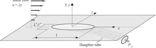
Figure 1. The flow configuration for streamlined branching of a relatively small daughter from a mother tube, with incident shear flow, in non-dimensional form.
the mother. The shaping in a healthy body is presumed to suppress or minimize the flow separations and adverse consequences which are otherwise prone to occur at these Reynolds numbers. Quantitative studies are few in this area and the flow structure interaction of distensible walls may also reduce separation. Similar aspects of wall shaping are met in the other applications, for example associated with the detailed flow inside a suction hole, where mother–daughter interaction is important for receptivity in connecting theory to experiments in the transition or control context (Maet al. 1999), and in the supply to car cooling systems.
Model investigations have been made for various branching-flow configurations. Those in Smith (1977), Bennett (1987), Brotherton-Ratcliffe (1987), Blyth & Mestel (1999) and Smith & Jones (2000) have relatively large daughter tubes and concern flow effects which are almost inviscid and are examined over relatively short streamwise length scales. While all the papers consider branching into two daughter tubes, Smith & Jones also consider arbitrarily many daughters, with a view to the understanding of flow through arteriovenous malformations. Slow flows are studied by Tutty (1988). Direct numerical simulations and experiments include those described by Caro et al. (1996), and Hademenos, Massoud & Vi˜nuela (1996), who also address the malformations mentioned above. Work on graft–artery junctions in Lei, Kleinstreuer & Archie (1997), Loth et al. (1997), Paz et al. (1992), Sherwin et al. (2000) and Doorly et al. (2002) is also relevant though the focus of the latter work is on flow from branch to main vessel. By contrast, studies of small side branches with mother– daughter interaction and moderate or comparatively high flow rates appear to be rare.
1.2. Motivation and model problem
theory sheds light on the question of how the influence of the downstream pressure in the daughter branch can travel upstream and mate with the mother-flow pressure properties outside.
The theory concentrates on relatively high Re values while direct simulations are for moderateRe. It is hoped that the theory which is strictly valid only forRe → ∞ applies at finite values of Re, an aspiration for which the direct simulations can provide a check. Agreement at moderateRevalues between theory, direct simulations and experiments in pipe and channel flows is shown in Dennis & Smith (1980), Smith (1979), Sobey (1980), Durst & Loy (1985), Mei & Plotkin (1986) and Bhattacharyya, Dennis & Smith (2001). To begin, the present model problem is introduced and the theory for planar steady flow is considered, in § §2–4. The theory is then extended to planar unsteady flow in§5.1 and to three-dimensional flow (with symmetry-plane results) in§5.2.
We show that the ‘mating’ of the daughter-branch pressure with the mother pressure occurs through a very rapid change over a very short streamwise length scale in the pressure and velocity at the mouth of the daughter. This abrupt pressure ‘jump’ is supported by the combination of solid wall (underneath) and flow shear (on top). If a relatively small overall pressure drop is imposed the flow response hinges on interactive wall-layer behaviour with negligible outer displacement, giving the flow solutions in both the mother and the daughter. A higher pressure drop, considered in §5.3, yields a stronger ‘jump’ which produces a feedback of displacement to the wall layer outside the branch and forces the branch mouth to act as a point or line sink. The feedback is favourable upstream, where it counters, in terms of flow separation, the disadvantages of wall shape in the lead-up to the daughter opening. Downstream the feedback is adverse and can drag back some mother fluid particles that have streamed past the opening and then deposit them into the daughter branch. Section 6 presents further comments.
2. The flow structure of the model problem
We begin with the problem of steady flow at relatively largeRe. Consider a slender side branch situated in a fixed wall and lying deep inside the incident wall layer or other shear flow in the mother tube, figure 1. Relative to the entrance to the branch, the wall appears flat and infinitely long (thex-axis), while the fluid appears to be of semi-infinite extent in the normal direction, with uniform shear flow upstream. The only relevant geometric length scales are those of the daughter branching itself; thus we take a typical streamwise length of the branching from its inception to its opening as the characteristic streamwise length scale ∗ of the local flow, so that this length has a non-dimensional value of 1. In the three-dimensional case shown in figure 1, L∗ signifies a typical spanwise length scale.
Restricting our attention to two dimensions (figure 2) for the present, we assume that the above length scale ∗ is large compared with the typical normal extent (h∗ say) in a slender side branch. As there is no velocity scale u∗, we take the prescribed slope λ∗ of the incident velocity profile at the surface multiplied by ∗, leaving u∗ =λ∗∗ as the velocity scale based on the branch length.
Non-dimensional quantities are to be used, so that the streamwise and normal Cartesian coordinates are ∗(x, y) respectively, the corresponding fluid velocity is
Shear flow
Y, y
Region (i) Region (ii)
Region (iii)
x a1
f1
(x1)
f4
f2
f3
1
Figure 2. As in figure 1 but for steady or pulsatile planar motion, showing the viscous regions (i)–(iii) and the wall shapesf1–f4.
turn the density and kinematic viscosity of the incompressible fluid. The aim in this and the next section is to construct a solution of the continuity and Navier–Stokes equations for largeRe.
2.1. Governing equations for relatively large Re
At such large Reynolds numbers, and assuming there is no significant separation, the viscous effects required to enforce the no-slip condition only operate in a thin layer near the wall. The width of the viscous layer and the equations that describe it follow from an order of magnitude analysis of the Navier–Stokes equations. Thus we require inertial forces (∼u2/x) to balance the viscous forces (∼Re−1u/y2). With the assumption of a linear velocity profile near the wall (u∼y) and taking the x length scale to be unity, it follows that the viscous-layer width scales asRe−1/3. Therefore the critical branch thicknessh∗ is comparable withRe−1/3∗for nonlinear effects (such as a near separation) to play a substantial role, and the typical branch slopes involved are of order Re−1/3. The representative value of u is also of size Re−1/3 while the induced pressurepscales withRe−2/3.
Throughout the wall layer, wherey=Re−1/3Y and x, Y areO(1), it follows that
(u, v, p) =Re−1/3U,Re−2/3V ,Re−2/3P,
and the viscous-layer equations of continuity and streamwise momentum,
U =ΨY, V =−Ψx, (2.1a, b)
U Ux+V UY =−P(x) +UY Y, (2.1c)
govern the flow in terms of order-one quantities. HereΨ (≡Re2/3
is continuous from mother to daughter, with f1, f4 equal at x1± while downstream f2>f3> f4 because of the divider thickness and the open daughter branch.
For the computations we consider as specific choices forf1 tof4 the following:
f1 =−h1x2, 06x 6x1,
f2 =h2(x−x1)2(2 +x1−x)2, x1 6x 62 +x1,
f3−f4=h1x12, x>x1.
(2.2)
Here the middle equation for the shapef2, although restricted tox 62 +x1 for the present work, could be extended to largerx values if necessary, depending on where the downstream boundary condition on the mother flow is set. The starting condition upstream represents the undisturbed state,
U →Y, V →0, P →0 as x→ −∞. (2.3a)
The boundary conditions for all the flow outside the branch, in regions (i) and (ii) of figure 2, are
U =V = 0 at Y =
f1(x) for x < x1, (2.3b)
f2(x) for x > x1, (2.3c)
U −Y →0 as Y → ∞, (2.3d)
for no slip and no far-field displacement respectively. The constraint of zero displacement at large normal distances in (2.3d) applies here because the current representative streamwise length scale is much less than the representative thickness of the whole large-scale incident flow of which U in (2.3a) gives the relatively near-wall part. The flow inside the branch in the daughter region (iii) must satisfy the no-slip conditions
U =V = 0 at Y =f3(x), f4(x), for x > x1. (2.4a, b)
In addition the fluid pressure is prescribed at a downstream station inside the daughter branch, written asx2 say, with x2> x1. So
P−=P∞ at x=x2 (2.4c)
for the side-branch flow (iii), where P∞ is a given constant pressure level, taken to be less than the upstream level of zero. The superscripts ± where used are to distinguish between flow quantities above and below the divider in regions (ii) and (iii) respectively.
The mass flux entering the branch (iii) from the mother (i) is a basic unknown (corresponding to Ψ = C, an unknown constant, on Y = f3(x)) and depends on the downstream pressure level imposed in (2.4c). It is directly related to the relative heighta1 of the dividing streamline and is measured from the initial divider level for convenience.
2.2. Conditions on the pressure
The explanation concerns the starting conditions for regions (ii) and (iii), and the flow very close to the branch opening, which has a non-parabolic nature and allows upstream influence to enter. The latter flow provokes a streamwise ‘jump’ in pressure and velocity across the branch opening (the daughter entrance) in general, when viewed from the order-one scale of x, i.e. there is a very rapid change over a very short length scale. The strength of that ‘jump’ at the upstream end of the branch depends on (2.4c) prescribed at the downstream end. Thus the Kutta-like condition (2.4c) downstream is accommodated by means of an upstream influence which spreads to the branch opening (although no further than that) and which indeed is at its most rapidly varying at the branch opening. This is the most unusual aspect of the present branching flow structure.
In more detail, the interior of the ‘jump’ at the branch opening involves a local region of small extent O(Re−1/3) in both the streamwise and normal directions. The interior velocities areO(Re−1/3) from continuity and from the incident flow speeds in region (i), and so the typical pressure isO(Re−2/3). Thus here
u∼v∼Re−1/3
, p∼Re−2/3
, withx−x1=Re−1/3X.
Hence the response here is mainly inviscid and the interior controlling equations are the Euler equations, forX∼1. These lead to conservation of the scaled mass flux and vorticity along the streamlines of the interior region, with the vorticity distribution being determined by the shear ∂U/∂Y incident from the longer-scale region (i) upstream at x = x1−, and likewise for the mass flux. The appropriate boundary conditions include those of tangential flow at the solid walls, which locally appear parallel (at Y = f1(x1) throughout and at Y = f2(x1) = f3(x1) over a semi-infinite streamwise range). So in effect
Ψ = 0 at Y =f1(x1) for allX,
Ψ =C at Y =f2(x1) =f3(x1) for X>0,
where the branching starts at X = 0. The additional requirements are of matching upstream to the incident velocity and pressure from (i) at x1−, and matching in the far field toΨ ∼ 12Y2+O(1). The flow is assumed to enter and leave this Euler region unidirectionally but with an overall displacement of its streamlines and hence its vorticity distribution and pressure, consistent with the above boundary conditions, and with smooth attached flow in between. Substantial separation is excluded. It is assumed that the no-slip condition at the flat bottom of the Euler zone along Y = f1(x1) is satisfied by means of an attached thin viscous sublayer, and similarly along both sides of the divider Y = f2(x1) = f3(x1), subject only to minor local separations at most. Fuller details are analogous with those in Bowles & Smith (2000), see also Smith & Jones (2000), Jones & Smith (2003). Again, these induced viscous sublayers form downstream the beginnings of the Blasius-like effects on the longer scale described in the next subsection.
Vorticity conservation is equivalent here to the classical Bernoulli property on the scaled pressure. Thus from the conditions holding at the upstream and downstream ends of the interior Euler region we have the requirements
at x=x1±
Ψ is conserved along streamlines, (2.5a)
P +1
2U
2 is conserved along streamlines, (2.5b)
P(f1)
0 0.5 1.0 1.5 2.0 2.5 0
–2 × 10⁴
x
Jump
P(f4)
P(f3)
P(f2)
Pressure
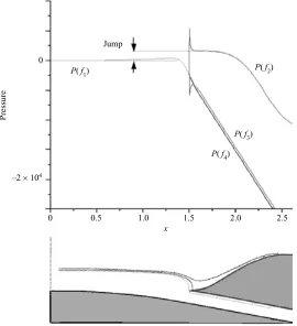
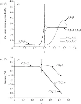
Figure 3.A direct simulation for the geometry (2.2) with a prescribed mass-flow shift or relative heighta1= 0.625. HereRe= 222.
opening, in order to satisfy (2.4c) further downstream. The conditions also reflect the fact that the value C of Ψ at the inner divider wall f3 is unknown in advance (whereasΨ is zero alongf4), corresponding to the unknown mass flux entrained into the branch from the oncoming motion upstream.
Whilst the theoretical development preceded the computational work (the latter is to be discussed fully in§4), we illustrate the very rapid change in pressure which occurs even at moderate Re by showing figure 3, for the purpose of motivation. Figure 3 presents the variation in pressure along the mother and daughter surfaces f1 tof4. The computation is for Re = 222 with a scaled daughter mass flow corresponding to a relative heighta1 = 0.625; see also §4. For this condition, the stagnation point is a very short distance along the upper divider surface f2 from the opening as can be seen from the plot of the stagnation streamline and two neighbouring streamlines below the pressure curves. The rapid variation in pressure is clear.
2.3. How the pressure ‘jump’ is accommodated by the flow structure
at large Y throughout the ‘jump’ and outside it. It follows that the displacement constraint (2.3d) can be maintained across the ‘jump’. By contrast, a uniform velocity in the far field would be insufficient to support such a pressure ‘jump’, at least from region (i) to region (ii). (Incidentally, the exact solution for the Euler flow in the interior of the ‘jump’ is identical to that of Jones & Smith (2003) if the incident profileU at x1− is entirely linear. Their physical setting and that in Smith & Jones (2000) are quite distinct from the present configuration, however. Smith & Jones consider a set of larger daughter tubes in predominantly inviscid flow, without the present engulfing of a daughter tube by near-wall shear flow). Again, the streamwise ‘jump’ can arise only at the branch opening, not inside the branch (iii) or in the outside flow (i) and (ii), or at a trailing edge in the case of a graft-like configuration. The overall flow problem is inherently nonlinear and requires computation (§3). We suppose the lead-up (region (i)) to the branch opening to be not so severe as to provoke separation and hence as discussed in§2.2 there is no upstream influence ahead of the opening. Also, the scaled pressure along the lowermost wall is taken to fall across the ‘jump’ , so thatP− atx=x1+ is less than the value ¯P ofP atx=x1−, to keep the flow attached there. The pressure ‘jumps’, which leave ¯P =P+ = P− in general at the stationx1,also leave the starting profilesU for the regions (ii) and (iii) non-zero next to the wallsf2, f3, f4 and therefore induce a Blasius-like development just beyondx1. This development has to be accommodated in the computations. The non-zeroU value at the lowermost wall in particular is [2( ¯P −P−)]1/2 atx
1 in view of the ‘jump’ (2.5b).
2.4. Limiting analysis
Increasingly negative values of the scaled end pressure P∞ correspond to increased suction into the branch. Then the relative height a1 of the dividing streamline is expected to become large, for a fixed branching shape, as the amount of oncoming fluid drawn from the mother tube into the daughter branch increases. In consequence, at the ‘jump’ most of the incident vorticity (shear) is unity and the velocity profile is predominantly linear. Hence there is some simplification, as follows.
First, ifU±,π± denote the scaled streamwise slip velocities on the divider and the pressures just downstream of the ‘jump’, respectively, and U = U0 is the oncoming velocity profile from region (i), then the general ‘jump’ conditions from (2.5a, b) yield
π++ 1 2(U
+)2=π−+ 1 2(U−)
2= ¯P +1 2U
2
0(Y0), π−+12U 2 w= ¯P .
HereY0=f2(x1) +a1 gives the dividing streamline position andUwis the slip velocity induced locally at the lowermost wall f4 for x = x1 +. For large values of P∞ the velocity profile above the divider must be unaltered to leading order, because of (2.3d). This implies thatU+ is negligible, andU
0 is approximatelyY. Also, sincea1 is large andf2(x1) is onlyO(1),Y0 is approximatelya1. So the above gives
π+ ∼P¯+ 12a21 (2.6)
to a first approximation. Underneath the divider, at the entry to the daughter branch, the near-unit shear requires a velocity profileY−f4(x1)+Uwand thereforeU−=h+Uw with h denoting the initial branch width (f3 −f4)(x1). Eliminating the pressure difference gives the balancea12= (U−)2−U2
w,which ish2+ 2hUw. However, because a1 is large andhof order one,
must be large. Hence also, from the above equations,
π− ∼ −1 8a
4
1h−2 (2.8)
is very large. It is interesting that the pressure rise π+ in (2.6) is associated with bringing fluid as if to rest just on top of the divider, with the mother flow in (ii) then being an undisturbed shear motion in effect (as if without any branching at all). In contrast, the pressure fall π− in (2.8) is produced by an effectively uniform entry motion into the daughter, of speed given by (2.7) to preserve the mass flux. The predictions (2.6)–(2.8) are found to be close to the computational results, as figure 4 below shows.
Second, because the streamwise approach to fully developed motion in the daughter is often fast, conservation of mass and momentum directly between the branch opening atx1+ and the end station x2 now points to the predictions
(π−−P∞) = 6a21(x2−x1) h3, τ−= 3a21 h2 (2.9)
for the approximate pressure drop and wall shear along the daughter branch, respectively. The upper and lower wall shears of the daughter are approximately the same. Here (2.9) applies provided the daughter width is unchanged, P∞ and a1 are large and the distance x2−x1 is not too small. The predictions in (2.9) also agree with the computational results below. The wall shear here is−1
2hP(x). We observe that the trends in (2.6)–(2.9) involve an unusual combination of high- and low-inertial flow features.
3. Solution for planar steady branching properties at largeRe
The flow in each area (i)–(iii) was resolved numerically with a finite-difference procedure similar to those in Smith & Timoshin (1996) and Bowles & Smith (2000). A Prandtl transposition, withY−fn(n= 1,2,4 respectively), replacedY for convenience, and in area (iii) the transposedY was also normalized with the local daughter branch thickness f3−f4. The procedure applies three-point centred differencing in Y and three-point backward differencing in x, for (2.1c), and similarly for (2.1a, b). This yields the velocities and pressure at a discrete station x implicitly from the known solutions at the two previous stations. Forward motion with U positive is assumed. Second-order accuracy inx as well as Y is obtained by solving the implicit equations iteratively. The solution behaviours immediately after the branch-opening ‘jumps’ (i.e. at x = x1+) are accommodated by two-point streamwise differencing to cover the first step only; the solutions are found to merge closely with the Blasius forms there. The solution is marched forward successively through (i) and then separately through (ii) with (2.3c, d) holding and through (iii) with (2.4a, b) holding. Typical grids used have x, Y steps of 0.005, 0.02, with a transposed Y range of 10, and finer grids were adopted as checks.
0 1 2 3 10
20 30
0 1 2 3
–60 –40 –20 0 20
(a) (b)
(c) (d)
x x
(i)
(ii) (iii)
(iii)
a1 = 2.8125
a1 = 0.5625
P
r
r (i)
(iii)
(iii) (ii)
(ii) a1 = 2.8125
a1 = 2.8125
0 2 4 6 8 0 1 2 3 4
2 4 6 8
U– (a
1 = 0.5625) Y – f
U–(a
1 = 2.8125) U+ U0
–120 –80 –40 0 40
a1
r r
π+
r
π–
P_
Figure 4.Steady planar-flow results for the wall shaping (2.2). (a, b) Shear τ (at walls
f1, f2, f4) and pressuresP , P+, P−versusx, in regions (i)–(iii) respectively, for two values of
a1. (A close-up of the results in (i) is contained in figure 12a.) (c) The velocity profiles on either side of the ‘jump’ atx1, for the two values ofa1used in (a, b). (d)P∞,π± plotted against a1. Herex2= 2.625. Comparisons with (2.6)–(2.9) (denoted byr) are included.
velocitiesU±(at the divider) atx1+ in view of (2.5b). Here the normal compression or expansion of the velocity profile in order to satisfy (2.5a, b) is handled computationally by interpolation. Then, given a1, the flow solutions for the velocities and pressures in areas (ii) and (iii) are marched forward to the downstream ends, in particular to x=x2 in the daughter branch (iii). There the pressure solution P− is compared with the end value (2.4c). An overall iteration on a1 can be performed to satisfy (2.4c) directly but in practice the inverse procedure of setting a1 and then deducing the associatedP∞ value is far more productive here, given that the relationship between a1 andP∞ is found to be single-valued.
slopes in the lead-up shapef1and within (ii) for shapesf2that produced excessive flow divergence. The ‘jumps’ across the branch-opening stationx1are apparent throughout, followed by viscous-layer growth on each side of the divider just downstream and an often rapid approach thereafter to fully developed flow within the daughter branch. The divider starts at Y = 0, x = x1. Again, the flow solution in (iii) depends only on f3−f4, not on the individual shapes f3, f4, and so the daughter (iii) could be curved or straight for instance. The values x1 = 1.5, x2 = 2.625, h1 = 12, h3 = 3 are taken. In figure 4(a, b) the flow solutions, for shifts a1 = 0.5625 and 2.8125, show the wall shear reducing in the lead-up region (i) under an induced adverse pressure gradient. After that the mother flow in (ii) attaches firmly to the front of the constriction f2 with a favourable pressure gradient and increased wall shear, before tending towards detachment beyond the maximum constriction point and then returning to undisturbed flow downstream. In the daughter (iii) the flow approaches the fully developed Poiseuille form downstream under a favourable induced pressure gradient. The flow in (i) is not affected by the value of a1, whereas that in (ii), (iii) clearly is affected. Figure 4(c) presents, for the two cases above, the velocity profiles U0,U±atx=x1±. These emphasize the velocity ‘jumps’ across the branch entrance. The increased response of the entry velocity u1 for the larger a1 value stands out. Figure 4(d) summarizes the properties found over a range ofa1orP∞values. It shows
π± and P∞ plotted againsta1, verifying that theP∞–a1 relation is single-valued, and it also compares with the analytical results (2.6)–(2.9).
4. Direct numerical simulations
4.1. Method
Direct numerical simulations of the Navier–Stokes equations were performed using the commercial package fluent(5.3) for the planar steady motions described above. The algorithm chosen utilized a second-order upwind variant of the well-known
simplepressure-correction method. The lower part of the computational domain was
defined by the functions f1 to f4 of (2.2) over the interval 0 6 x 6 2.625. The inflow velocity profile was specified as a constant shear, and the upper computational boundary was prescribed as a moving wall (zero normal displacement). Values for the outflow mass flux ratio between mother and daughter tubes were prescribed according to the required amount of deflection (a1) of the oncoming streamlines. Physical dimensions for the computational domain correspond to a height of 1.5 at the computational domain inflow, a length from inflow to the daughter tube (x1 in the theory) of 1.5, and an overall length of 2.625 in the x-direction. Using a value of kinematic viscosity ν = 1, the velocity on the top surface of the computational domain was prescribed to provide Reynolds numbers of either 500 or 222 based on the velocity slope (denoted λ∗ in the theory).
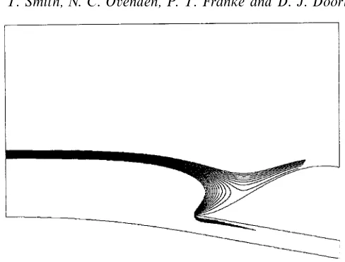
Figure 5. Tracks of 20 particles, half of which are released above the streamline corresponding toa1 + daughter height, fora1= 2.8125,Re= 222.
4.2. Results and comparisons
The results are presented in figures 5–8, for the branching shape of (2.2), together with comparisons, while figure 9 is to allow further comparisons with the theory to be made. The Reynolds numbersRe used in figures 6–8 are 222 and 500, which were set by taking∗, ν∗ andρ∗ as unity and prescribing the incident velocity slope λ∗ as 222 or 500. The streamline heighta1 imposed in these cases is either 2.8125 or 0.625, and the unscaled height of the daughter inlet is fixed at 0.1417 for all three cases.
In scaled terms accounting for the Re−1/3 factor the cases of figures 6–8 are associated in turn with values ofh1 equal to 0.3809, 0.3809 and 0.5 in the theory, with correspondinga1 values of 2.8125, 0.625 and 2.8125. So, whereas the case in figure 8 is covered by figure 4’s theoretical results, we include in figure 6 the theoretical results for h1 = 0.3809; for thath1 value the theoretical results in figure 6 are based on the
0 0.5 1.0 1.5 2.0 2.5 25
50 (a)
Scaled w
all shear stress (magnitude)
Theory Computation:
w(f1(x)), w(f4(x))
w(f2(x)), w(f3(x))
x
0
–25
–50
–75
–100
–125
0 0.5 1.0 1.5 2.0 2.5 3.0 (b)
Scaled pressure
Theory Computation:
P(f2), P(f3)
P(f1), P(f4)
Theory Computation:
P(f2)
P(f1)
x
0.5 1.0 1.5 2.0 2.5 –4
–2 0 2 4 6 8 10
(c)
x
Scaled pressure
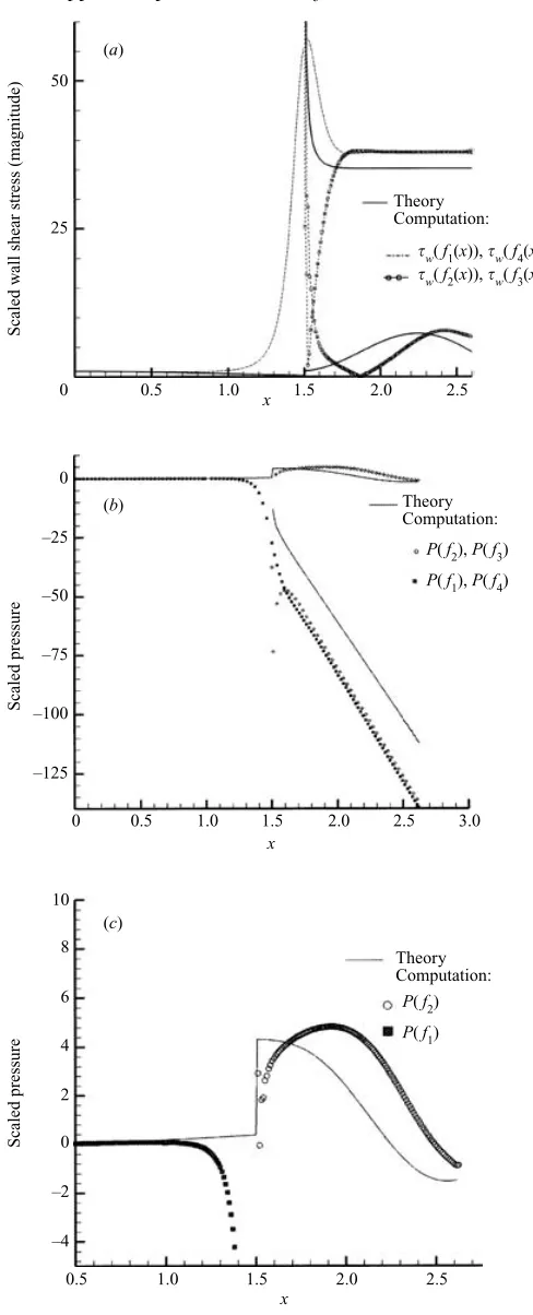
scaled wall shears and pressures whena1 is 2.8125. Figure 9 shows the scaled shears and pressures at the downstream endx2 in the daughter side-branch over a range of a1 values, accompanied by the two direct simulation results.
The comparisons are encouraging. There is good qualitative agreement on the general flow structure and on the wall shear and pressure responses throughout the mother and daughter flows. This adds credence to the pressure ‘jump’ phenomenon anticipated in the theory for increased Re. There is also evidence of both low and high suction pressure effects arising in the direct simulations. We consider further the qualitative and then quantitative aspects of the comparison next.
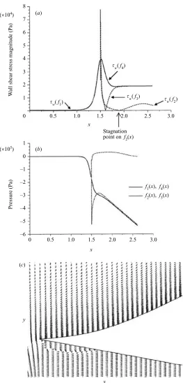
Figure 5 shows pathlines of particles released on either side of the flow dividing streamline fora1 = 2.8125, Re= 222. Note that for this value ofa1 the daughter tube acts as a significant sink, and there is a local region of backward flow entrainment from the mother which enters the daughter tube. Thus the boundary layer on the boundary f2 of the mother commences further downstream, beyond the stagnation point which occurs at approximatelyx= 1.9. This is clearly shown by the comparison of figure 6 below, where the form of the shear stress predicted by the theory agrees closely with the computation, but the latter curve appears shifted downstream to account for the displaced stagnation point. A similar phenomenon occurs in the cases of figures. 7 and 8 though to a lesser extent.
Figure 6 below also compares the pressure levels for the computation and theory and then shows in more detail the comparison of pressure predictions for the mother tube from theory and computation with a1 = 2.8125 and Re = 222. Agreement is good for the pressure variation in the mother tube; in the daughter tube, the high suction peak generated by the additional flow entrained backwards into the daughter produces an offset in the computational pressure results curve compared with the theoretical prediction, figure 6(b).
Now concerning the quantitative predictions, first we consider again the direct simulations in figure 6(a–c) which are for Re=λ∗ = 222,a1 = 2.8125, h1= 0.3809. The dimensional computations here have already been rescaled by (λ∗)4/3for pressure andλ∗ for wall shear stress. (Fuller details are presented in the caption to the figure.) The agreement can be seen to be quite good quantitatively. A significant sink effect is also evident, nevertheless, resembling that studied in§5.3 later.
Second, the simulation in figure 7(a, b) again has Re = λ∗ = 222, h1 = 0.3809 but a1 = 0.625. (The results here are not scaled, but rescaling could be performed as above.) With this lower mass flux entrained into the daughter, the stagnation point on the flow divider is still located on the outer wall, but is nearly on the apex of the divider. The wall shear and pressure (figure 7a, b) in the mother region (i) ahead of the branching here also show signs of the favourable influence of increased relative suction as described in§5.3, after the adverse geometrical influence further upstream. The wall shear initially decreases, then increases, in line with the theoretical predictions in figure 12 below. The overall pressure drop in the daughter implied theoretically if the increased suction effect is ignored is about 79% of that in the simulation, but allowing for the abrupt behaviour very close to the branch entrance in the simulation the percentage rises to about 99%. Again, the ratio of minimum pressure in region (ii) to that in (iii) is about 30% in both the simulation and the theory, and the end pressure and wall shear results at this a1 value are in keeping with the graph in figure 9.
0 (a)
w(f2)
x 0.5
0.5 1.0 1.5 2.0 2.5 3.0 1.0
1.5 2.0 2.5 3.0 3.5 4.0
(b) (×103)
W
all shear stress magnitude (P
a)
P(f2(x))
w(f4), w(f3)
f1(x), f4(x) f2(x), f3(x) w(f1)
P(f1(x))
P(f3(x))
P(f4(x))
–3.5 –3.0 –2.5 –2.0 –1.5 –1.0 –0.5 0 0.5 1.0 (×104)
Pressure (P
a)
0
x
0.5 1.0 1.5 2.0 2.5 3.0
Figure 7. As figure 6 but Re = λ∗ = 222, a1 = 0.625. (a) Wall shear stress magnitude distribution from computational solution of Navier–Stokes equations. Daughter flow rate is lower than for figure 6 and corresponds approximately to streamlines of figure 2. Stagnation point occurs nearly on the flow divider. (b) Wall pressure distribution from Navier–Stokes computation corresponding to (a). With the much lower proportional flow rate in the daughter, compared with figure 6, the pressure drop in the daughter is more comparable with that in the mother.
(a)
w(f4) (×104)
W
all shear stress magnitude (P
a)
f1(x), f4(x)
w(f1)
0 0.5 1
2 3 4 5 6 7 8
(b)
1.0 1.5 2.0 2.5 3.0
w(f3)
w(f2)
Stagnation point on f2(x)
–6 0 –5 –4 –3 –2 –1 0 1
0.5 1.0 1.5 2.0 2.5 3.0
f2(x), f3(x) (×105)
Pressure (P
a)
x
x
(c)
x y
_–
0 1 2 3 4 5
–400 –300 –200 –100 0 100
P_
a1
Figure 9. Further comparisons between simulations and theory: theoretical results whenh1 in (2.2) is 0.3809, for end shears τ∞− and pressuresP∞ in the daughter side branch (iii) as a1 varies. This includes the values from the simulations in figures 6 and 7, shown as circles.
ratio as the Reynolds number is increased. In consequence a marked increase in flow reversal is observed in the mother region (ii) above the daughter in that case; compare the simulation in figure 8(a–c) with the theory for region (ii) as depicted in figure 12(c) later.
5. Extensions to unsteady, three-dimensional or increased-suction flows
Virtually the same argument, structure and properties as in§2 hold also for locally unsteady flow (§5.1) and locally three-dimensional flow (§5.2) at high Re. Again, all flows also produce an inviscid Euler zone further out, of streamwise and normal length scale O(1), whose role thus far is linear and so is passive in response to the induced wall pressure alongf1, f2. This outer Euler zone however becomes nonlinear and active for stronger suction pressures (§5.3).
5.1. Planar unsteady flows
The theory extends to unsteady flows as follows, taking account of the branch-opening ‘jumps’ as well as testing the applicability of the results of§2.4 for increased suction pressures in the daughter branch.
The relevant scale for the time t∗ is 1/λ∗ times Re1/3, for (say) pulsatile motion upstream in the mother tube or pulsatile end pressure imposed in the daughter branch. Here t∗ = Re1/3T /λ∗. Then (2.1a, b), (2.3b–d) and (2.4a–c) continue to hold for the
Figure 8. Continued
0 1
20 40 60 80
2 3
(iii)
(i) (ii)
T = 0.4
0
0.8
x
–160 –120 –80 –40 0 40
0 1 2 3
T
0.8
(i) (ii)
(iii)
0.4
x
–15 –10 –5 0 5
0 1 2 3 4 5
T
0 1 2 3 4 5
–200 –150 –100 –50 0
50 _–
a1
π+, P++ r
r
r
r
P_ (a)
T
0 1 2 3 4 5
T
0 1 2 3 4 5
1 2 3 4
5 (b)
a1
π+, P++
P_ _–
/x
1–
–200 –150 –100 –50 0 50
π– P
T = 0
π–
T
(c)
a1
π+, P++
/x
1–
1.03 1.04 1.05 1.06 1.07
0 1 2 3 4 5
T
0 1 2 3 4 5
–1.0 –0.5 0 0.5 1.0 1.5
a1
P/x1–
π–
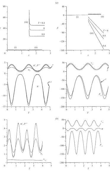
Figure 10. Unsteady planar-flow results for the shaping (2.2) withh2zero, from (5.1). (a) For prescribed a1(T) and steady input U ≡Y at x = 0. (b) For prescribed a1(T) and pulsating inputU atx= 0. (c) For a prescribedP∞ value (−30.666) and pulsating inputU atx= 0.
time-dependent unknowns with P∞ possibly depending on T , while (2.1c) must be enlarged to include a temporal derivative, giving
UT +U Ux+V UY =− ∂P
∂x(x, T) +UY Y. (5.1)
The upstream condition (2.3a) may be replaced depending on the incident motion. The branching geometry is assumed to be fixed. The jump conditions still apply exactly in the form (2.5a, b) because the balances within the short interior region surrounding x1 are quasi-steady over the present time scale. The relative height a1 which dictates the amount of mother fluid entering the daughter is now dependent on T, however. The unsteady flow here is supposed to be free of separation.
The computational method was extended to unsteady flow by use of a Crank– Nicholson procedure for marching in T, to preserve second-order accuracy. At each time level the spatial sweeping was performed much as for the previous steady case. The initial state was taken as a computed steady-flow solution, followed by time-marching which took steps of 0.004 typically.
Results for three representative unsteady forcings are presented in figure 10(a–c): (a) for pulsating end pressure P∞(T) or relative height a1(T) with steady incident mother flow; (b) for pulsating incident flow and a prescribed pulsating relative height a1(T); (c) for pulsating incident flow and a prescribed end pressure P∞(T). In cases (a) and (b) we prescribed a1(T) in order to find the end pressure needed to produce a given influx into the daughter, from a steady or unsteady mother flow. For case (c) the requiredP∞(T) variation was satisfied numerically by means of Newton–Raphson iterations on a1(T) at each time level. In figure 10(a–c) the wall shaping is as in (2.2) but with h1 = 13 and h2 = 0 to focus on unsteady rather than constrictional effects.
In more detail, figure 10(a) has the incident profileU =Y atx= 0,and the relative height a1 is prescribed as b1(1 +b2sinωT) with b1 = 2, b2 = 0.4, ω = π. The results show the wall-shear and wall-pressure distributions at selected times and the temporal evolution of the representative pressures π±, P∞, P+(2.4375) (denoted by P++) and wall shearτ−(x2) (denoted by τ−
and (iii) are always favourable but pulsate, and indeed all the branched flow appears to settle soon into a nonlinear pulsating state. The pulsating end pressureP∞ in (iii) is relatively large and negative, while in (ii) the spatial pressure variation is much less, as the closeness of π+, P++ indicates, because the velocity profile at the start of (ii) differs comparatively little from that of uniform shear (in line with large-a1 behaviour) andh2 is zero. In Figure 10(b) the incidentU is set as the pulsatile profile Y+b3sin(πT)Yexp(−Y), with b3 = 12, and a1 is prescribed as in figure 10(a) except that now ω = 2π. The solution soon acquires a doubly periodic form involving the two forcing frequenciesπ,2π, as the temporal variations ofπ±, P∞, and so on, show. Figure 10(c) is for the same incident pulsatile profile as in figure 10(b) but P∞ is prescribed as a constant. The solution for the relative height a1, as well as π±, etc., is shown versus T. The pulsations of a1 and of the wall shear in (i) at the branch opening are quite small compared with the majority of the pressure pulsations, due to the imposed uniform end pressure. Calculations have also been performed for other pulsing incident profiles and they lead to the same trends.
Stronger suction pressures −P∞(T) are again of interest, corresponding to large a1(T) values. Since the ‘jump’ properties remain quasi-steady the results in (2.6)–(2.8) continue to apply exactly then. The working approximation (2.9) also holds in many cases. Comparisons shown in figure 10(a) support the predictions (marked again by ‘r’) for large a1(T) values and enhanced suction pressures, and the results in figure 10(b, c) clearly have the same trend also.
5.2. Three-dimensional branching properties
Three-dimensional side-branching motion is described by virtually the same flow structure as in the planar case. Suppose first that the spanwisez∗ length scale L∗ of the branch is comparable with the streamwise one∗; see figure 1. Then the flow-structural argument applied in three dimensions, with a spanwise velocity component given by
w∗ =λ∗∗(Re−1/3
W+· · ·), with z∗=∗z,
leads to the controlling equations
Ux+VY+Wz= 0, (5.2a)
U Ux+V UY +W Uz=−Px(x, z) +UY Y, (5.2b)
U Wx+V WY+W Wz=−Pz(x, z) +WY Y, (5.2c)
instead of (2.1a–c). All the constraints in (2.3)–(2.4) continue to hold here provided x, zdependence is allowed for in f1 and f2, and W tends to zero in each condition (except possibly (2.4c) which is imposed on the pressure). The position x1 of the branch entrance and the suction pressureP∞ also depend onz in general.
The flow problem (5.2a–c) with (2.3)–(2.4) (extended as above) is a computational one which is very difficult to solve accurately, with or without separation, because of the extra spatial dimension and global nonlinear upstream influence. The latter is due to three-dimensional free interaction as in Smith (1976, 1983) and Smith, Sykes & Brighton (1977), additional to the upstream influence inherent in the ‘jump’, and it makes the flow problems elliptic both in the mother regions (i),(ii) and in the daughter region (iii) beyond the opening ‘jump’.
If the typical spanwise scaleL∗is large compared with∗ then thez-derivatives can be neglected in (5.2a, b), leaving the entire flow quasi-planar forU, V andP. Then the solutions of earlier sections apply, with nonlinear ellipticity being suppressed, while W follows from (5.2c) with negligible W Wz and with Pz given by the quasi-planar solution at eachz station.
Suppose instead that the spanwise scale L∗ is relatively small. This corresponds to a branch whose x, z planform is longitudinal in the streamwise direction, and whose y, z cross-section is closer to being round. Then the typical |W| is reduced in proportion, for continuity, and the spanwise variation in the pressure response likewise reduces for the spanwise momentum balance, while other quantities remain of order unity. Hence (5.2a–c) still control the flow but with noPx term in the mother regions (i),(ii); alsoPx is replaced in the daughter region (iii) by an unknown pressure gradient P0(x) which is independent ofz. The nonlinear ellipticity is suppressed for such longitudinal branching motion.
The flow calculation along a symmetry plane (z= 0 say) then becomes well-posed. There
W∼zW¯(x, y) say, and so the longitudinal motion reduces to the form
Ux+VY + ¯W = 0, (5.3a)
U Ux+V UY =−P0(x) +UY Y, (5.3b)
UW¯x+VW¯Y+ ¯W2 =−Q¯(x) + ¯WY Y. (5.3c) Here the velocity componentsU, V are evaluated atz= 0 and depend only onx and Y,while P0 is identically zero in (i),(ii) andzQ¯ signifies the unknown scaled spanwise pressure gradient. Three-dimensional flow is provoked by the short spanwise length scale, so that a substantial streamwise pressure gradient is precluded in regions (i),(ii) (but not in the contained region (iii)) as it would also act over larger spanwise scales there. Hence the streamwise pressure ‘jump’ P0 across x1 from (i) to (ii) affects the pressure level in region (ii) but not the pressure gradient there.
Numerical solutions of (5.3a–c) were derived subject to the extensions of the boundary conditions (2.3)–(2.4) mentioned earlier in this section. In particular ¯W is conserved along a symmetry-plane streamline as it passes across the ‘jump’ at the branch opening. The computational method used was an enlargement of that in§3.1 to accommodate the extra momentum equation (5.3c) and the linkage toU, V via the term ¯W in (5.3a), and similar meshes were employed.
x
(a)
1
0 1 2 3 0 1 2 3
–10 0 10 20 W all shear –10 0 10 20 –20 –10 x (i) (i) (ii) (iii) (ii) (iii) 2 1 1 2 2 (i) (ii) (iii) Q Pressure
P0′
x
0 1 2 3
–10 0 10 20 30 40 1 (i)
(i) 2 (iii)
(ii) 2 2 1 (ii) (iii) 1 (b) –80 x
0 1 2 3
–60 –40 –20 0 20 Q (ii) (iii) (i)
P0′
W
all shear Pressure
Figure 11.For three-dimensional branching flow: symmetry-plane results, from (5.3a–c), for the shaping (2.2). Wall shearsτ1, τ2,spanwise pressure contribution ¯Qand streamwise pressure gradientP0are shown versusx, in regions (i)–(iii), for (a)a1= 32,(b)a1= 3.
loss or gain of mass flux to or from the spanwise direction and hence interaction with the flow outside the symmetry plane. In the results shown here the flux represented by theY-integral of U across the gap in (iii) is set as constant, as just one example. Other results show that varying the flux can affect the downstream development in (iii) substantially. The flux issue does not arise in the mother flow of regions (i),(ii) because of the absence of an upper wall there.
is fora1increased to 3. This yields similar but accentuated behaviour, including higher wall shears and more favourable streamwise pressure gradients in (iii) with increased negative spanwise gradients acting, although the spanwise motion in (iii) changes from outward near the branch opening to inward further downstream. The relief of the motion into the spanwise direction causes interesting contrasts with the corresponding planar-flow results of figure 4, leaving the spanwise wall shear much less reduced from its incident value during the lead-up to branching in the current longitudinal case.
For large values of a1 the predictions (2.6)–(2.8) again hold good, accompanied by a re-scaling with respect to the pressure to account for the total longitudinal response.
5.3. Stronger suction pressures
Given that the results for large a1 and enhanced pressure drops apply whether the local branching flow is steady or unsteady, two- or three-dimensional, we consider further strengthened suction pressures next. The geometry is as before however and the steady planar case is again our focus.
New physical effects enter if the typical pressure drop in the mother flow streaming over the branching is increased to the size Re−1/3, as opposed to Re−2/3 in the previous theory. The reason is that, on the broader lateral scale of order unity in y mentioned earlier, inviscid velocity perturbations ofO(Re−1/3) must be induced; these perturbations include a wall slip velocity of that same order, which therefore violates the implied assumption in (2.3d) of a much smaller slip velocity. This increased pressure is produced by the relative height a1 increasing to the order Re1/6 in view of (2.2), so that the y-scale of entrained fluid rises toRe−1/6a2 with a2 now of order unity. Thus here
u−y∼p∼Re−1/3,with entrainedy=Re−1/6a2 [in mother].
Along with this, (2.7) and (2.8) suggest that the pressuresπ− andP∞ in the daughter (iii) both increase by a factor Re2/3, although the difference between them is not so large. The increase of typical pressures in (iii) is such that, with the present strengthened suction, the unscaled pressure values p immediately after the opening ‘jump’ and at the downstream end of (iii) become of order unity. So, in contrast with the preceding equation, here
p∼1 [in daughter].
These perhaps surprisingly large pressures are generated because the entry velocity into the O(Re−1/3) thick daughter just beyond the ‘jump’ is uniform and must be of O(1) magnitude (in fact, 12a2
2h−1); this magnitude is required to accommodate the O(Re−1/3) mass flux ψ of all the fluid below the dividing streamline whose distance from the lowermost wall is of orderRe−1/6. Further, the downstream end pressureP
∞ can now be identified with the value−1
8a 4
2h−2 since the difference between the entry and end pressures within the daughter is small.
The broaderO(1) inviscid region is taken to remain immersed in the incident shear flow (u=y) of the mother, so that there is no influence from an uppermost wall for example. Then the present suction level provokes an O(Re−1/3) perturbation in the stream function, say Re−1/3˜
ψ, forcing an expansion of the form
[u, ψ, p] =y,12y2,0+Re−1/3[˜
u,ψ,˜ p˜] +· · · (5.4a)
vorticity, subject to boundedness in the far field and to the wall conditions of zero ahead ofx=x1 but of a positive uniform valueK(= 12a22) beyondx1. The uniformity ofK is due partly to the strong abrupt entrainment into the daughter (as if into a point sink) via the jump at the branch opening and partly to the lack of any geometrical effect from either of the wall shapesf1orf2 in this comparatively large-scale inviscid region. Specifically, K = 1
2a 2
2 from extension of §2.4 and since ¯P is negligible. The solution for ˜ψ is simply K[π−tan−1(y/(x−x1))]/π, and the resultant slip velocity near the wall is thereforeRe−1/3 timesK/(π(x1−x)).This is positive upstream of the daughter and negative downstream, in line with an acceleration towards the branch opening in both cases.
Hence the wall-layer description now remains as in (2.1), (2.3) except that (2.3d) is replaced by
U −Y → K
π(x1−x)
as Y → ∞ (5.4b)
because of the extra induced slip from the strong suction. Reduced suction lessens K, leaving the upstream influence ahead of the branch insubstantial as before. With K being of order one and positive, however, (5.4b) represents a favourable effect on the upstream flow that counters the adverse one from the lead-up shape f1 seen earlier. Compare the effects in Smith (1978) and Ovenden (2001). Indeed, a Prandtl transposition shows the solution to depend only on the difference function
K/(π(x1−x))−f1(x), (5.5)
implying that the suction-pressure effectK is bound to dominate sufficiently close to the branch opening, irrespective of whether the wall shapef1 dominates upstream.
The numerical results in figure 12(a, b) for region (i) confirm the influence of the suction parameter K. They show in particular the wall-layer flow becoming very attached as x approaches x1 from upstream. The response there is analysable as in Smith (1978), as is the increase of upstream influence when the value ofK increases. This is in line with the difference function (5.5). In particular, figure 12(a) shows the wall shearτand pressureP for the branching lead-up shape in (2.2) withh1 = 12 again andK varying from zero to 2. The increasingly favourable effect onτ andP is such that forK = 2 the wall shear produced always exceeds the incident upstream value. Figure 12(b) has h1 increased to 1, which forces the lead-up flow to separate when K is zero. Higher K values however suppress the separation and lead to responses similar to those in figure 12(a). On the other hand, downstream in region (ii) for x > x1 the suction-pressure effectK is adverse and indicates flow reversal occurring. The geometrical effect of the wall shape, here f2, enters in a fashion similar to that in (i), but the upper half of the starting velocity profile for (ii) has a uniform shear (in view of the estimates in§2.5) added to the K term exactly as in (5.4b) where U is positive. This forces the lower half of the starting flow in (ii) to be reversed and unknown. Some mother fluid therefore passes into region (ii) beyond the openingx1 but is then decelerated and drawn back into the ‘jump’ region and thence into the branch (iii). See results in figure 12(c). The internal structure of the ‘jump’ itself
x
(a)
–3 –2 –1 0 1 2
0 2 4 6 8
0 1 2 2 K = 1
x
–3 –2 –1 0 1 2
–8 –6 –4 –2 0 2
K = 0
P
1 2
1 2
x
–3 –2 –1 0 1 2
0 2 4 6 8
Separation 2
K = 4
–2
0
x
–3 –2 –1 0 1 2
–8 –6 –4 –2 0 2
K = 0
P
1
2 4 (b)
(c)
–10 –8 –6 –4 –2 0 2 4
0 2 4 6 8 10
Y
U x –
x1 = 0.1
0.15
0.20 0.25 1
then needs more study although this may disturb the current ‘jump’ conditions very little, a matter addressed in Ovenden (2001). The upstream and downstream influence spreads monotonically, over distances ∝ K3/4, as the suction-pressure parameter K continues to increase.
6. Further comments
How the pressure adapts was one of the main motivations for the present work. For the lower pressure drops studied prior to §5.3, the work highlights the importance of the branch entrance region where a rapid local streamwise variation or ‘jump’ occurs in the induced pressures and velocities. In that region local to the entrance the upstream influence from the daughter branch begins, and the mother–daughter interaction is concentrated. This holds whether the motion is steady or unsteady, two- or three-dimensional. The ‘jump’, which generates an abrupt rise in pressure in the streamwise mother-tube flow but an abrupt fall into the daughter, is the key to explaining the influence of the daughter end pressure.
The other main motivation was to compare direct numerical simulations with the theory. The present comparisons (§4.2) point to reasonable agreement at moderate Reynolds numbers Re, as well as confirming the rapid variation in flow properties implied by a ‘jump’ at the branch entrance, at suchRe values.
For the higher pressure drops of §5.3, the corresponding strengthened suction not only draws increased amounts of mother fluid into the daughter but also yields additional upstream influence, stretching into the mother flow ahead of the branching. The feedback effect is favourable and opposes the adverse effects of the upstream wall shaping. This is encapsulated in the difference function (5.5). Further increased pressure drops yield enhanced upstream and downstream influence. These in particular should prevent upstream separation from arising, even for negative and positive slopes of order unity in the respective wall shapes ahead of and beyond the side branching (e.g. with a tube dilation ahead followed by constriction beyond). An analogue of the feedback effect of §5.3 applies also for unsteady and three-dimensional flows as in § §5.1,5.2, due to the quasi-planar quasi-steady nature of the ‘jump’. Sufficiently strong pulsations however lead to finite-time breakdown (Li et al. 1998), while in three-dimensional motion fluid can enter the daughter branch from the sides.
numerical challenge as described in §5.2. The crossover, between mother fluid that does and does not enter the daughter branch, is passive towards the spanwise edges of the branch but the crossover positions are unknown in advance. More understanding of separation in these branching flows also represents a challenge, particularly of the structure of the ‘jump’ process with reversed flow at the daughter entrance.
Thanks are due to Dr. C. Atkin for his interest and encouragement, to Dr. A. Seifailian for suggesting certain references, and to EPSRC and DERA Farnborough for support of N.C.O. through a CASE award.
R E F E R E N C E S
Bennett, J. M.1987 Theoretical properties of three-dimensional interactive boundary layers. PhD
thesis, University of London.
Bhattacharyya, S., Dennis, S. C. R. & Smith, F. T. 2001 Separating shear flow past a
surface-mounted blunt obstacle.J. Engng Maths39, 47–62.
Blyth, M. G. & Mestel, A. J. 1999 Steady flow in a dividing pipe. J. Fluid Mech. 401,
339–364.
Bowles, R. G. A. & Smith, F. T. 2000 Lifting multi-blade flows with interaction.J. Fluid Mech. 415, 203–226.
Brotherton-Ratcliffe, R. V. 1987 Boundary layer effects in liquid layer flows. PhD thesis,
University of London.
Caro, C. G., Doorly, D. J., Tarnawski, M., Scott, K. T., Loy, Q. & Dumoulin, C. L.1996
Non-planar curvature and branching of arteries and non-Non-planar-type flow.Proc. R. Soc. Lond.A
452, 185–197.
Dennis, S. C. R. & Smith, F. T.1980 Steady flow through a channel with a symmetrical constriction
in the form of a step.Proc. R. Soc. Lond.A372, 393–414.
Doorly, D. J., Sherwin, S. J., Franke, P. T. & Peir ´o, J.2002 Vortical flow structure identification
and flow transport in arteries.Comput. Meth. Biomech. Biomed. Engng5(3), 261–273.
Durst, F. & Loy, T.1985 Investigations of laminar flow in a pipe with sudden contractions of cross
sectional area.Computers Fluids13, 15–36.
Ellis, J. E. & Poll, D. I. A.1996 Laminar and laminarizing boundary layers by suction through
perforated plates. InSecond European Forum on Laminar Flow Tech., Bordeaux, June 10–12, 1996, pp. 8.17–8.27.
Hademenos, G. J., Massoud, T. F. & Vi˜nuela, F.1996 A biomathematical model of intracranial
arteriovenous malformations based on electrical network analysis: theory and hemodynamics.
Neurosurgery38, 1005–1015.
Jones, M. A. & Smith, F. T.2003 Fluid motion for car undertrays in ground effect.J. Engng Maths
(in press).
Lei, M., Kleinstreuer, C. & Archie, J. P.1997 Hemodynamic simulations and computer-aided
designs of graft-artery junctions.J. Biomech. Engng119, 343–348.
Li, L., Walker, J. D. A., Bowles, R. I. & Smith, F. T. 1998 Short-scale break-up in unsteady
interactive layers: local development of normal pressure gradients and vortex wind-up.
J. Fluid Mech.374, 335–378.
Lighthill, M. J.1972 Physiological fluid dynamics: a survey.J. Fluid Mech.52, 475–497.
Loth, F., Jones, S. A., Giddens, D. P., Bassiouny, H. S., Glagov, S. & Zarins, C. K. 1997
Measurements of velocity and wall shear stress inside a PTFE vascular graft model under steady flow conditions.J. Biomech. Engng119, 187–194.
Ma, B., van Doorne, C. W. H., Zhang, Z. & Nieuwstadt, F. T. M.1999 On the spatial evolution of
a wall-imposed periodic disturbance in pipe Poiseuille flow atRe= 3000. Part 1. Subcritical disturbance.J. Fluid Mech.398, 181–224.
Mei, R. W. & Plotkin, A. 1986 Navier–Stokes solutions for laminar incompressible flows in
forward-facing step geometries.AIAA J.24, 1106–1111.
Olufsen, M. 1999 Arterial modelling: from data to real time simulation. Presentation, ICIAM Conference, Edinburgh, 5–9 July 1999.
Ovenden, N. C. 2001 The effect of increasing localized suction on a boundary layer and the
generation of horseshoe vortices. PhD thesis, University of London.
Paz, D.1997 Numerical model and experimental investigation of blood flow through a bifurcation.
Interaction between an artery and a small prosthesis.ASAIO J.43, 326–333.
Paz, D., Einav, S., Elad, D. & Avidor, J. M.1992 Numerical model of blood flow through a
bifurcation: interaction between an artery and a small prosthesis.Med. Biol. Engng Comput. 30, 543–550.
Pedley, T. J.1995 High Reynolds number flow in tubes of complex geometry with application to
wall shear stress in arteries. InBiological Fluid Dynamics(ed. C. P. Ellington & T. J. Pedley). Pub. Co. of Biol. Ltd.
Peir ´o, J.1999 Simulation of blood flow using high-order spectral elements on unstructured grids.
Presentation,ICIAM Conference, Edinburgh, 5–9 July 1999.
Sherwin, S. J., Shah, O., Doorly, D. J., Peir ´o, J., Papaharilaou, Y., Watkins, N., Caro, C. J. & Dumoulin, C. L. 2000 The influence of out-of-plane geometry on the flow within a distal
end-to-side anastomosis.J. Biomech. Engng122(1), 86–95.
Smith, F. T.1976 Pipeflows distorted by non-symmetric indentation or branching.Mathematika23,
62–83.
Smith, F. T.1977 Steady motion through a branching tube.Proc. R. Soc. Lond.A355, 167–187. Smith, F. T.1978 Flow through symmetrically constricted tubes.J. Inst. Maths Applics.21, 145–156. Smith, F. T.1979 The separating flow through a severely constricted symmetric tube.J. Fluid Mech.
90, 725–754.
Smith, F. T. 1983 Properties, and a finite-difference approach, for interactive three-dimensional
boundary layers.Utd Tech. Res. Center Rep, pp. 83–46.
Smith, F. T. & Jones, M. A.2000 One-to-few and one-to-many branching tube flows.J. Fluid Mech. 423, 1–31.
Smith, F. T., Sykes, R. I. & Brighton, P. W. M. 1977 A two-dimensional boundary layer
encountering a three-dimensional hump.J. Fluid Mech.83, 163–176.
Smith, F. T. & Timoshin, S. N.1996 Blade-wake interactions and rotary boundary layers.Proc. R. Soc. Lond.A452, 1301–1329.
Sobey, I. J.1980 On flow through furrowed channels.J. Fluid Mech.96, 1–26.