Computational Techniques to Predict Orthopaedic Implant Alignment and Fit in Bone

(1)

Scholarship@Western

Electronic Thesis and Dissertation Repository

4-23-2014 12:00 AM

Computational Techniques to Predict Orthopaedic Implant

Alignment and Fit in Bone

Seyed Kamaleddin Mostafavi Yazdi The University of Western Ontario Supervisor

Dr. Remus Tutunea-Fatan

The University of Western Ontario Joint Supervisor Dr. James Johnson

The University of Western Ontario

Graduate Program in Mechanical and Materials Engineering

A thesis submitted in partial fulfillment of the requirements for the degree in Doctor of Philosophy

Follow this and additional works at: https://ir.lib.uwo.ca/etd

Part of the Biomechanics and Biotransport Commons

Recommended Citation Recommended Citation

Mostafavi Yazdi, Seyed Kamaleddin, "Computational Techniques to Predict Orthopaedic Implant Alignment and Fit in Bone" (2014). Electronic Thesis and Dissertation Repository. 1998.

https://ir.lib.uwo.ca/etd/1998

This Dissertation/Thesis is brought to you for free and open access by Scholarship@Western. It has been accepted for inclusion in Electronic Thesis and Dissertation Repository by an authorized administrator of

(2)

(Thesis format: Integrated)

by

Seyed Kamaleddin Mostafavi Yazdi

Graduate Program in Mechanical and Materials Engineering

A thesis submitted in partial fulfillment of the requirements for the degree of

Doctor of Philosophy

The School of Graduate and Postdoctoral Studies The University of Western Ontario

London, Ontario, Canada

(3)

ii

Abstract

Among the broad palette of surgical techniques employed in the current orthopaedic

practice, joint replacement represents one of the most difficult and costliest surgical

procedures. While numerous recent advances suggest that computer assistance can

dramatically improve the precision and long term outcomes of joint arthroplasty even in the

hands of experienced surgeons, many of the joint replacement protocols continue to rely

almost exclusively on an empirical basis that often entail a succession of trial and error

maneuvers that can only be performed intraoperatively. Although the surgeon is generally

unable to accurately and reliably predict a priori what the final malalignment will be or even

what implant size should be used for a certain patient, the overarching goal of all

arthroplastic procedures is to ensure that an appropriate match exists between the native and

prosthetic axes of the articulation.

To address this relative lack of knowledge, the main objective of this thesis was to

develop a comprehensive library of numerical techniques capable to: 1) accurately

reconstruct the outer and inner geometry of the bone to be implanted; 2) determine the

location of the native articular axis to be replicated by the implant; 3) assess the insertability

of a certain implant within the endosteal canal of the bone to be implanted; 4) propose

customized implant geometries capable to ensure minimal malalignments between native and

prosthetic axes. The accuracy of the developed algorithms was validated through

comparisons performed against conventional methods involving either contact-acquired data

or navigated implantation approaches, while various customized implant designs proposed

(4)

iii

It is anticipated that the proposed computer-based approaches will eliminate or at least

diminish the need for undesirable trial and error implantation procedures in a sense that

present error-prone intraoperative implant insertion decisions will be at least augmented if

not even replaced by optimal computer-based solutions to offer reliable virtual “previews” of

the future surgical procedure. While the entire thesis is focused on the elbow as the most

challenging joint replacement surgery, many of the developed approaches are equally

applicable to other upper or lower limb articulations.

Keywords

Computer-assisted surgery; total elbow arthroplasty; flexion-extension axis; implant

malalignment; humerus; computed tomography; insertion trajectory; implant design;

(5)

iv

Co-Authorship Statements

Chapter 1: Kamal Mostafavi - sole author.

Chapter 2: Kamal Mostafavi - study design, analysis, wrote manuscript; Evgueni

Bordatchev – data collection, reviewed manuscript; James Johnson – study

design, reviewed manuscript; Remus Tutunea-Fatan – study design, reviewed

manuscript.

Chapter 3: Kamal Mostafavi - study design, analysis, wrote manuscript; Emily Lalone –

data collection, reviewed manuscript; Graham King - study design, reviewed

manuscript; James Johnson – study design, reviewed manuscript; Remus

Tutunea-Fatan- study design, reviewed manuscript.

Chapter 4: Kamal Mostafavi - study design, analysis, wrote manuscript; James Johnson –

study design, reviewed manuscript; Remus Tutunea-Fatan – study design,

reviewed manuscript.

Chapter 5: Kamal Mostafavi - study design, analysis, wrote manuscript; James Johnson –

study design, reviewed manuscript; Remus Tutunea-Fatan- study design,

reviewed manuscript.

(6)

v

Acknowledgments

I would first and foremost like to thank my supervisors Dr. Remus Tutunea-Fatan and Dr.

James Johnson. During my Ph.D they have always supported and encouraged me to progress

in my research. I would also like to thank them for dedicating their time for having individual

weekly meetings, their great comments and contribution in my research and toward

progressing my thesis. They always provided invaluable feedback in every single step of my

work and helped me in various ways to solve the issues I faced during this research.

I would like to further thank Dr. Tutunea-Fatan for his great contribution during my research,

for his time that spent every single day from the beginning of my research and being a

wonderful supervisor all the time supporting me.

I would also like to thank Emily Lalone for her great support in providing information and

data on specimens all the time and also helping me in understanding this information and

answering my questions. Thank you to Colin McDonald for his great feedbacks and support

through the experimental setup and corresponding information.

At the end I would like to thank my lovely wife, Fatemeh, for always being there for me and

providing love, support and guidance and helping me a lot during my Ph.D. Thank you to my

mom and dad who dedicated their lives to their children. You are my inspiration and my

(7)

vi

List of Tables

Table 2.1: The comparison of the proposed B-Spline method against uniform, chordal and

centripetal methods ... 62

Table 3.1: Quantitative comparisons between B-Spline and voxel-based methods ... 102

Table 5.1: Summary of the best three implant designs with minimum malalignment

developed by the stem-focused optimization method. ... 177

developed by the spool-focused optimization method. ... 177

developed by the overall implant optimization method. ... 178

(12)

xi

List of Figures

Figure 1.1: Elbow anatomy: (a) anterior view of right arm, showing the three elbow bones:

humerus, radius and ulna, and (b) the three joints of elbow: radiohumeral, humeroulnar and

radioulnar joints. ... 4

Figure 1.2: Anterior view of the distal humerus. ... 6

Figure 1.3: Motion of the elbow: (a) flexion-extension movement, and (b)

supination-pronation movement. ... 8

Figure 1.4: X-ray of a total elbow arthroplasty. ... 11

Figure 1.5: (a) 3D representation of distal humerus acquired by CT scanner, and (b) the distal

humerus cross section in transverse, sagittal and coronal planes. ... 14

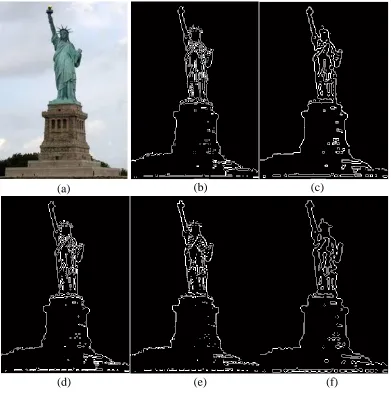
Figure 1.6: Comparison of different edge detection techniques; (a) original sample image,

adapted from [http://en.wikipedia.org/wiki/Statue_of_Liberty], (b) Prewitt, (c) Canny, (d)

Sobel, (e) Roberts, and (f) LOG methods. ... 18

Figure 1.7: (a) Anatomical features of the native elbow joint, and (b) elbow joint after total

elbow arthroplasty with prosthetic components. ... 20

Figure 2.1: Segmentation of the bone contours: a) overall positioning of the analyzed axial

CT slice, b) raw DICOM image of the axial slice, c) thresholded outer and inner bone

contours, and d) detailed bone contour data points... 44

Figure 2.2: 2D pixel intensity mapping in CT slices. ... 46

Figure 2.3: Bone contours extracted through the proposed approach from representative: a)

middle, and b) extreme distal cross sections of the humerus. ... 47

Figure 2.4: Comparison of the proposed segmentation (blue and green contours) against

conventional edge detection methods: a) Canny, b) Prewitt, c) Laplacian of Gaussian, d)

(13)

xii

Figure 2.5: Parametric formulation of a closed B-Spline. ... 51

Figure 2.6: Control polygon deformation through global modification. ... 56

Figure 2.7: Control polygon deformation through local modification. ... 58

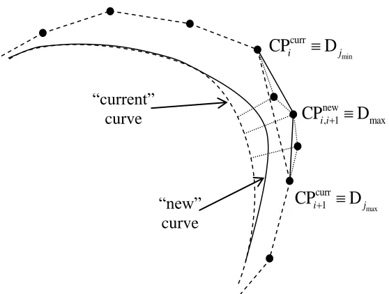
Figure 2.8: Closed B-Spline fitting through control polygon deformation: a) to ..) global modification; …) to h) local modification. ... 59

Figure 2.9: Local behavior of closed B-Spline approximants: a) outer, and b) inner bone

contours. ... 60

Figure 2.10: Graphical comparison between the tested closed B-Spline fitting methods. ... 63

Figure 2.11: Pair-wise registration of two correlated point datasets. ... 66

Figure 2.12: Separation of humeral fragment of interest: a) approximate location of detached

humeral segment within the overall distal humerus, and b) detail view of the reduced humeral

specimen. ... 69

Figure 2.13: Typical cross sections through reduced humeral specimen as obtained in

principal CT planes. ... 70

Figure 2.14: Contact data acquisition setup: a) overview of Kugler CNC measurement

system, and b) kinematics of the measurement process. ... 72

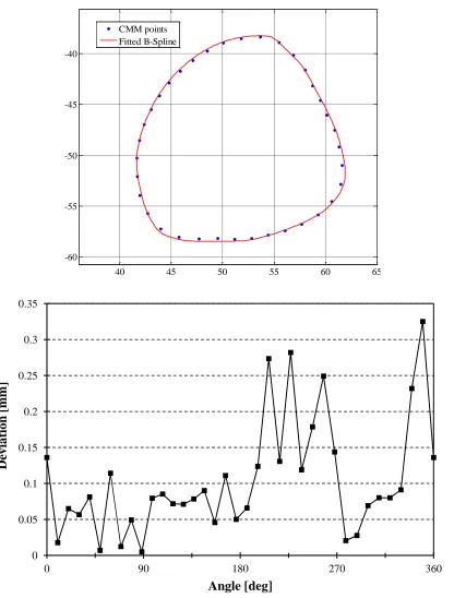
Figure 2.15: Comparison between contact-acquired data and proposed bone reconstruction

method: a) CMM point dataset, b) B-Spline fitting technique, and c) overlay of the two

datasets. ... 74

Figure 2.16: Deviation between reconstructed geometry and contact-acquired data: a) sample

of relative positioning between CMM points and parametric curves; and b) variation of the

deviation around outer contour circumference. ... 76

Figure 3.1: Anatomical position and orientation of the flexion-extension axis: (a) medial, (b)

(14)

xiii

Figure 3.2: Representative axial cross sections through distal humerus: (a) raw CT slices, and

(b) parametric curve-approximated outer bone contours. ... 88

Figure 3.3:Progressive adaptation of the fitted B-Spline curve shape: (a) initial set of

segmented CT points, (b) approximating curve after one global modification iteration (one

Step 2), (c) approximating curve at the end of the global modification phase (end of Step2),

and (d) final shape of the approximating curve (end of Step 3). ... 95

Figure 3.4: Sample of local curvature pattern along distal humeral B-Splines. ... 96

Figure 3.5: Determination of the geometric characteristics of FE axis through least squares

fitting. ... 98

Figure 3.6: Qualitative comparisons between the resulting point datasets obtained through

B-Spline (green) and conventional (blue) approaches achieved through: (a)-(d) combined fitted

features and bone overlay, (e)-(h) direct result overlay. ... 102

Figure 4.1: : Latitude implant configurations: (a) unlinked, and (b) linked versions ... 115

Figure 4.2: Implant Components: (a) small, medium, large and X-large spool sizes, (b)

anterior, centered and posterior offset spools, (c) different stem locations based on offset

spools, and (d) small, medium and large stem sizes. ... 117

Figure 4.3: 3D representations of the humeral implant and the distal humerus: (a) Latitude

humeral portion components containing humeral implant, spool and screw, and (b) anterior

view of the distal humerus. ... 118

Figure 4.4: Relative position of Latitude humeral implant in: (a) medial-lateral (ML) view (b)

anterior-posterior (AP) view of the distal humerus, and (c) 3D model of implant position in

medullary canal of the humerus. ... 120

Figure 4.5: (a) Implant penetration into the humerus due to improper fitting, and (b) 3D

model of implant penetration, showing interference areas in red. ... 121

Figure 4.6: Reconstruction of the distal humerus geometry: (a) DICOM images of the

(15)

xiv

images using developed control polygon technique, and (c) full 3D model of the humerus

from contours. ... 122

Figure 4.7: Reconstructed bone model: (a) control polygon form and (b) selection of three

critical cross sections as the GA input. ... 125

Figure 4.8: Selection of two distal and proximal ends of humeral implant stem as the GA

input. ... 126

Figure 4.9: Genetic algorithm iteration in generating populations and selecting proper. ... 127

Figure 4.10: Bone and implant coordinate systems: (a) three critical bone cross sections in

local Bone Coordinate System (BCS) and implant position in local Implant Coordinate

System (ICS). BCS is located in centroid of bone bottom cross section while ICS is at the

implant capitellum center, and (b) Implant position in BCS. In order to position the implant

in initial position for GA technique, the centroid of implant bottom cross section should

match the centroid of bone top cross section. ... 128

Figure 4.11: Implant Coordinate System (ICS) orientation with respect of Bone Coordinate System (BCS) over: (a) θ rotation about XBCS axis, (b) ω rotation about YBCS axis, and (c) ϕ

rotation about ZBCS axis. ... 129

Figure 4.12: Geometric interpretation of implantation malalignment: (a) 3D view of implant

position in bone cavity showing the translation error dCC, (b) anterior-Posterior view of

implant insertion showing varus-varus angulation error αVV, (c) medial-lateral view of

implant insertion showing flexion-extension angle αFE and (d) distal-proximal view of

implant insertion showing internal-external angulation error αIE. ... 132

Figure 4.13: Implant insertion procedure using GA technique: (a) 3D view of the humeral

implant from initial to final position, and (b) intermediate steps of implant insertion. ... 135

Figure 4.14: Schematic presentation of GA algorithm. ... 136

Figure 4.15: Validation of the developed method results in comparison with experimental

setup results: (a) implant alignment error in translation (mean + 1 standard deviation) for

(16)

xv

three directional components of medial-lateral (MED) error, anterior-posterior (ANT) error

and proximal-distal (PROX) error while Total represents square root of error components,

and (b) implant alignment error in rotation (mean + 1 standard deviation) for both developed

method and experimental setup. Rotational malalignment was reported in two components of

varus-valgus (VV) error and internal-external (IE) error while Total represents square root of

error components in rotation. ... 138

Figure 4.16: Definition of minimum implant distance to bone: (a) d1 to d4 represent the

distances of each implant corner to bone inner boundary in one cross section while d1

denotes the minimum implant distance to bone, (b) relation between slice numbers and bone

model, and (c) minimum implant distance to bone in each cross section from distal to

proximal end of the bone. ... 141

Figure 4.17: Definition of area ratio: (a) A1 denotes implant area while A2 represents bone

area delimited within the parametric definition of bone inner boundary in one cross section,

(b) relation between slice numbers and bone model , and (c) Area ratio of implant to bone

behaviour from distal to proximal end of bone. ... 143

Figure 4.18: Impact of implant/spool size change in objective function value and final

implant position ... 145

Figure 4.19: Repeatability test: (a) implant alignment error in translation (mean + 1 standard

deviation) for developed method starting from the same implant position in 5 runs, and (b)

implant alignment error in rotation (mean + 1 standard deviation) for developed method

starting from the same implant position in 5 runs. ... 146

Figure 4.20: Sensitivity to initial implant position in the developed GA technique: (a) implant

alignment error in translation (mean + 1 standard deviation) for developed method starting

from different implant orientation in 5 runs, and (b) implant alignment error in rotation

(mean + 1 standard deviation) for developed method starting from different implant position

and orientation implant position in 5 runs. ... 148

Figure 5.1: Stem-focused optimization variables: (a) Stem Coordinate System (SCS) located

in the centroid of distal implant cross section, and (b) and (c) represent two translational and

(17)

xvi

Figure 5.2: Spool-focused optimization method representation: (a) change in the position of

the capitellum and trochlea centers of the current shape of the implant, (b) current design of

the implant with its FE axis, and (c) new design for the implant distal part (where spool is

attached) with new FE axis. ... 165

Figure 5.3: Overall implant optimization method representation: (a) change in the positions

of the capitellum and trochlea centers and also centroids of the distal and proximal cross

sections of stem for current shape of the implant, (b) current design of the implant with its

current FE axis and current stem shape and (c) new design for the implant with new FE axis

and new stem shape. ... 168

Figure 5.4: Schematic chart of the first three methods (stem-focused, spool-focused and

overall implant optimization) for optimizing the shape of the implant. ... 171

Figure 5.5: Customized implant design method representation: (a) finding the proper 3D axis

that represents the largest common area of the bone cross sections, and (b) the resultant

envelope along the 3D axis. ... 174

Figure 5.6: Comparison of the developed implant design in the stem-focused optimization

method versus current design (green): (a) 3D view, and (b) side views of this comparison

implant designs. ... 180

Figure 5.7: Comparison of the developed implant design in the spool-focused optimization

Figure 5.8: Comparison of the developed implant design in the overall implant optimization

Figure 5.9: Comparison of the developed implant design in the customized implant design

(18)

xvii

Figure 5.10: Comparison of the four developed implant designs versus current design

(green): (a) 3D view, and (b) side views of the comparison of all implant designs. ... 184

(19)

Chapter 1

1

Introduction

1.1 Overview

This introductory chapter reviews elbow anatomy, elbow disorders and total elbow

arthroplasty. This chapter also highlights the challenges involved in total elbow

arthroplasty.

1.2 Joints and Implants

Joints articulate with bones of the human body and are responsible for movement. Joints

can be classified functionally and structurally based on the range of motion and type of

joint, respectively. Functionally, joints can be classified into three classes; 1) synarthrosis

joints with no movement, (2) amphiarthrosis or joints with slight amount of movement,

and (3) diarthrosis or freely movable joints. The last group of joints such as the elbow,

knee, shoulder and hip are more prone to different dislocations and injuries.

Orthopedic implants are incorporated to restore normal kinematic and range of

motion of the diseased joint. Although employing these implants reduces the pain and

replicate the motion of the damaged joint, they may loosen, wear or break in place.

Proper and efficient positioning of an implant into the cavity of the bone of a joint, not

only contributes to suppressing all these defects, but it also helps to reform the normal

functional joint.

In the recent years, computer-assisted surgery has been employed clinically in

some centers for the placement of the implants to improve the accuracy and precision of

(20)

movable joints of the human body vary markedly in terms of degrees of freedom,

complexity, overall size, bone structure and also canal shape. The current research which

investigates the interaction between the implant and bone focuses on the elbow joint and

the humeral canal with a more kinematic complexity, complicated canal shape and

smaller size. However, the general methodology related to implant-bone contact/collision

of this research is applicable to all other joints of the body.

1.3 Elbow

1.3.1 Anatomy and Biomechanics

The elbow joint, one of the most complicated joints of the body, connects the upper arm

to the forearm [Bernardino, 2010]. The humerus of the upper arm, and the ulna and radius

from the forearm, are three bones that form this synovial hinge joint. Structurally, the

elbow joint is a synovial joint, while functionally behaves as a hinge joint. As a synovial

joint, which is the most common and movable type of joints in human body, the elbow is

capable of achieving movement at the contact point of the articulating bones. In order to

ease this movement, articular cartilage covers the surfaces of the bones where they meet

and acts as a smooth substance which protects the bones during movement. As one of the

characteristics of synovial joints, all remaining surfaces inside the elbow joint are also

covered by a thin smooth tissue, called synovial membrane. Muscles, ligaments, and

tendons hold the elbow structure together to provide stability.

The human elbow is comprised of 3 articulations/joints; The humeroulnar joint in

which trochlear notch of the ulnar articulates with trochlea of the humerus, the

(21)

articulates with capitulum of the humerus, and the radioulnar joint in which the head of

the radius articulates with radial notch of the ulna (Figure 1.1). Although there are three

joints performing in the elbow, they provide two different motions only. The first two

joints (humeroulnar and radiohumeral joints) are in fact two hinge joints, which together

function as a hinge joint, providing flexion-extension movement for the elbow, while the

radioulnar joint is a pivot joint and responsible for supination-pronation motion.

Traditionally, the two hinge joints of the elbow are considered as the representation of the

elbow because the major task of the joint is to properly place the hand in space, while the

radioulnar joint does not have any share in this functionality [Palastanga and Soames,

(22)

Humerus

Ulna Radius

Radiohumeral joint

Humeroulnar joint

Radioulnar joint

(a)

(b)

Figure ‎1.1: Elbow anatomy: (a) anterior view of right arm, showing the three elbow bones: humerus, radius and ulna, and (b) the three joints of elbow: radiohumeral, humeroulnar and radioulnar joints.

(23)

The humerus is the longest bone in the upper limbs consisting of a body and two

extremities, which connects to shoulder joint from upper (proximal) side and to the elbow

joint from lower (distal) side. The body is composed of a cylindrical compact cortical

bone, thicker at the center while the structure of the two extremities is cancellous tissue

covered by a thin and compact layer. The cylindrical shaft contains an inner endosteal

medullary canal that runs along the length of the diaphysis. Cross-sections of the humerus

for both the periosteal shaft and medullary canal are not circles since the humerus is

wider in medial-lateral direction rather than in anterior-posterior, especially close to the

elbow.

The inner shape of endosteal canal is significantly important in positioning of the

humeral implant during elbow replacement surgeries. On the other side, the lower

extremity (distal) of the humerus plays a crucial role in surgical exposures since it

contains several anatomical features that help surgeons to identify native regions of the

elbow joint. These landmarks include two lateral and medial epicondyles which are

located on each side of the distal humerus, two articular surfaces which are capitellum

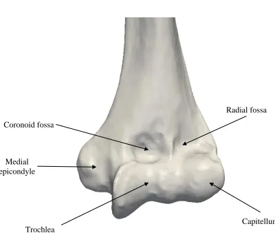
and trochlea, and three fossae comprised of the radial fossa, coronoid fossa and olecranon

fossa (Figure 1.2). The articular surfaces are a bit lower than (distal to) the epicondyles.

The lateral portion of the articular surfaces is a smooth rounded feature named the

capitellum, while the medial part is a hyperbolic concaved surface, named the trochlea,

which is separated by a groove called the trochlea sulcus. The capitellum articulates with

the radius to form the radiohumeral joint. The trochlea of the humerus articulates with the

ulna to represent the humeroulnar joint [Morrey and Bryan, 1982]. As reported

(24)

of the load applied to the hand is transmitted through the radiohumeral joint and the rest

is transmitted through the humeroulnar joint [Bernardino, 2010].

Medial epicondyle

Capitellum Trochlea

Coronoid fossa

Radial fossa

(25)

1.3.2 Motion and kinematics

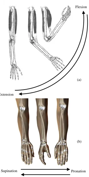
The motions of the elbow joint consists of the flexion-extension movement provided by

the humeroulnar and radiohumeral hinge joints and the pronation-supination movement

provided by the radioulnar pivot joint (Figure 1.3). The flexion-extension motion occurs

over an axis of rotation which is in fact the axis of the elbow hinge joint. In order to study

the exact location of this axis, concurrent study of the centers of motions for both

engaged joints (humeroulnar and radiohumeral joints) is required. The center of motion

for the humeroulnar joint was reported to coincide with the center of trochlea sulcus arc

for the majority of the flexion-extension range of motion, while the center of motion for

the radiohumeral joint was reported to almost match the center of capitullum arc. As a

result, the flexion-extension axis is a unique line that passes through arc centers described

by trochlea sulcus and capitellum, except at extremes of flexion and extension [London,

(26)

Figure ‎1.3: Motion of the elbow: (a) flexion-extension movement, and (b) supination-pronation movement.

Adapted from [http://www.eorthopod.com/content/adolescent-osteochondritis-dissecans-of-the-elbow; http://www.arn.org/docs/glicksman/eyw_040901.htm]

Extension

Flexion

Supination Pronation

(a)

(27)

1.3.3 Disorders

The study of biomechanics of the elbow can help surgeons to plan surgeries and apply

suitable treatments in difficult clinical problems, similar to other joints of the body. Many

routine activities highly depend on the performance and functionality of the elbow joint,

which is affected by both osseous and soft tissue structures. In the occurrence of different

types of disorders, the large ranges of motion are subject to significant losses and they

can impair the functionality of the elbow [Amis et al., 1982]. There are three major

groups of elbow disorders consisting of different types of arthritis, tumors, fractures, and

dislocations.

Arthritis involves inflammation in the joint. Swelling, joint stiffness, difficulty

with moving the joint, and muscle ache are other symptoms. One typical treatment option

with overall satisfactory results for patients with osteoarthritis is total elbow arthroplasty,

however, depending on the age and stage of the disease other treatment options might be

recommended [Baksi, 1998; Throckmorton et al., 2010]. Fractures can also lead to joint

replacement. Radial head and neck, olecranon, coronoid, the distal humerus, and condylar

fractures are common elbow fractures. In adults radial head fracture is the most common

fracture, while distal humerus fracture can be more challenging in elderly patients,

especially when associated with previous damages such as rheumatoid arthritis [Antuna

et al., 2012]. As one of the first studies, Cobb et al. [Cobb and Morrey, 1997] suggested

total elbow arthroplasty for elderly patients with the distal humerus fractures and reported

successful results after the surgery. As a result, replacement surgeries are more and more

accepted for the elbow as the use of hip replacement surgeries for elderly patients with

(28)

of complications for open reduction and internal fixation, total elbow arthroplasty as a

treatment decision for extensively comminuted fractures of the distal humerus is highly

recommended. The rate of this type of surgery for these patients is increasing due chiefly

to the rise in elderly population [Ali et al., 2010].

1.4 Medical Imaging

Medical Imaging is an important tool in the diagnosis and planning for joint replacement.

There are different methods, processes and instruments involved in creating the medical

images, among which X-ray, Computed Tomography (CT), Magnetic Resonance

Imaging (MRI), and ultrasound are the most common techniques.

1.4.1 Radiographs

In the X-ray technique, a source emits X-rays to the human body and on the other side a

recording film produces X-ray images from the patient. Depending on the absorption rate

of the different parts of the body, rays are absorbed or reflected and therefore the

X-rays that reach the recording film make the film dark. In this way, the recording film

records the attenuation of the X-rays, passing through human body. The resolution of the

image depends on the amount of energy generated by X-ray source, tube current, and

(29)

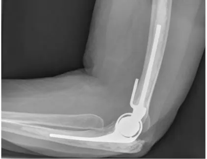
Figure ‎1.4: X-ray of a total elbow arthroplasty.

(30)

1.4.2 Computed Tomography

Computed Tomography (CT) is a non-invasive medical examination procedure that uses

specialized X-ray equipment to produce cross-sectional images of the body. The

difference between CT and ray is that CT produces multi-sliced 3D images, while

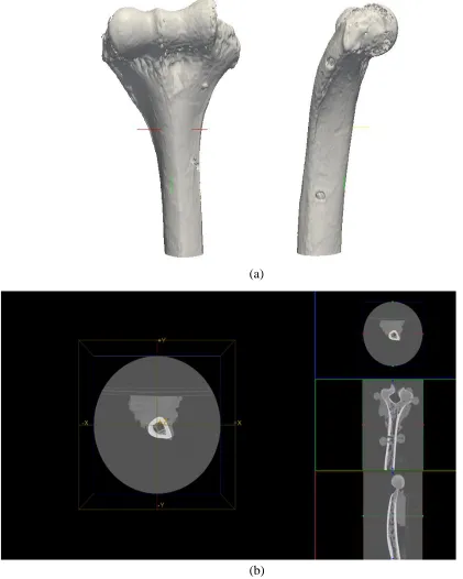
X-ray is a 2D representation of the human body (Figure 1. 5). In this technique, a detector

rotates around the patient and as a result takes images at different angles. All the images

are processed and reconstructed into multiple cross sectional (slices) images. Obviously,

3D image comparing to a 2D image delivers larger amount of information.

In orthopedics-related CT applications [Wang, 2009], accurate representation of

the endosteal cavity of the humerus is a mandatory and preliminary step for positioning

of the humeral implants during total elbow arthroplasty. Furthermore, this information is

critical in determination of optimized implant stem. This calls for an accurate geometric

representation of the cortical bone as one of the decisive premises of successful

reconstruction.

1.4.3 Digital Imaging and Communication in Medicine (DICOM)

In 1983, the American college of Radiology (ACR) and National Electrical

Manufacturers Association (NEMA) introduced the first standard named Digital Imaging

and Communication in Medicine (DICOM), capable of storing, handling, and

transmitting information in medical imaging. DICOM became the global format for

(31)

different scanners, work-stations, and servers from multiple manufacturers into a Picture

Archiving and Communication System (PACS).

Each DICOM file contains grids of pixels which depending on the density of the

tissue forms a grayscale spectrum (Figure 1.5). One of the applications of DICOM files in

orthopedics field is to extract the 3D geometry of the bone from a stack of DICOM slices.

In order to accomplish this, pixels belonging to outside and inside boundaries of the

cortical bone are detected in each single DICOM file and then these boundaries are

(32)

(b) (a)

(33)

1.4.4 Edge Detection Methods

Edge detection aims at identifying points/pixels in a digital image at which sharp changes

in image intensity occurs. Edge detection techniques benefit from a set of mathematical

methods to locate the boundaries of objects within an image which are characterized by

abrupt discontinuities due to change in image brightness [Nadernejad et al., 2008; Maini

and Aggarwal, 2009]. Edge detection filters and keeps important structural properties

(i.e., boundaries of objects). Detecting the edges/boundaries is an essential step in image

segmentation and image reconstruction. All the methods in edge detection employ either

gradient-based method which searches for maximum or minimum in first derivative of an

image, or Laplacian-based technique which employs zero crossings in the second

derivative of an image.

Canny, Sobel, Prewitt, Robert, and Laplacian of Gaussian are the major edge

detection techniques in image processing. The Canny edge detector method [Canny,

1986] is known as the standard technique. The Canny algorithm is based on converting

the edge detection problem into a signal processing optimization problem in which there

is a minimum deviation between the distance of the edge pixels, found by the algorithm,

and the actual edge [Canny, 1986; Maini and Aggarwal, 2009]. As the first step of this

algorithm, the Canny algorithm smoothens the image with a two-dimensional Gaussian to

eliminate the noise, and then calculates the gradient of the image in both directions to

identify regions with high spatial derivatives. Since edges occur at points where the

generated gradient is a maximum, Canny applies a non-maximum suppression to

eliminate non-maximum pixels. Canny then uses high and low thresholds (named as

(34)

simple 3*3 convolution kernels to create a series of gradients in both x and y directions.

These magnitudes of gradients are plotted at the end to represent edges/boundaries of an

image. The main characteristic of Sobel technique is that it is incredibly sensitive to

noises in images. Prewitt technique [Seitz et al., 2010; Shirvakshan, 2012] is similar to

the Sobel algorithm in terms of kernels involved in generating gradient values. Unlike

Sobel technique, the Prewitt operator is a fast operator that does not put emphasis on

pixels that are close to the center of the masks and therefore it is only suitable for

well-contrasted noiseless images. The Roberts algorithm [Roberts, 1965] benefits from 2*2

convolution kernels to calculate 2D spatial gradient measurements. The Roberts

technique highlights regions of high spatial frequency which at the end correspond to

edges. The most common use of this technique is its application on grayscale images as

input and output [Shirvakshan, 2012]. Laplacian of Gaussian function known as LOG

function employs a smoothening filter, performed by convolution with a Gaussian

function and followed by a derivative operation. The LOG operator is a 2D isotropic

measure of the 2nd derivative of an image, which is sensitive to noises [Juneja and

Sandhu, 2009].

It is really essential to understand the differences between different edge detection

techniques, their advantages, disadvantages, and their special applications (Figure 1.6).

Typically, gradient-based algorithms such as Prewitt are sensitive to noise although they

might work faster than others. It is reported in [Juneja and Sandhu, 2009] that under

noisy conditions, Canny, Robert, and Sobel represent better performance respectively.

The other factor, which is important, is the quality of output images, which under these

(35)

methods. Canny algorithm depends heavily on adjustable factors such as standard

deviation for the Gaussian filter and threshold values. Although Canny method is

computationally more expensive comparing to the others, it performs accurate edge

detection on images [Miani and Aggarwal, 2009; Juneja and Sandhu, 2009; Nadernejad et

(36)

Figure ‎1.6: Comparison of different edge detection techniques; (a) original sample image, adapted from [http://en.wikipedia.org/wiki/Statue_of_Liberty], (b) Prewitt, (c) Canny, (d) Sobel, (e) Roberts, and (f) LOG methods.

(b)

(d)

(c) (a)

(37)

1.5 Total Elbow Arthroplasty

Total Elbow Arthroplasty (TEA) involves replacement of the damaged elbow joint with

artificial components (implants) aiming at restoring elbow function and relieving pain in

the patient (Figure 1.7). Operatively, surgeons identify the native articulation axis and

remove diseased portions of the elbow and then prosthetic replacement is performed for

the humeral and ulnar sides. Implant stems are inserted into the medullary canals of the

corresponding bones and fixed by cement while surgeon ensures the flexion-extension

axis best matches the native articulation axis of the elbow [Brownhill, 2007]. The implant

configuration/alignment inside the bone canals affects the kinematics and load transfer of

the elbow after surgery. The crucial issue here is to replicate the same kinematics and

load transfer system as accurate as possible to avoid potential failure [Bauer and Schils,

(38)

Native flexion-extension axis

Capitellum _Medial

edpicondyle

Radial head

Lateral edpicondyle

Trochlea sulcus

sulcus

Humeral stem

Implant flexion-extension axis

(a) (b)

Figure ‎1.7: (a) Anatomical features of the native elbow joint, and (b) elbow joint after total elbow arthroplasty with prosthetic components.

(39)

1.5.1 Surgical Techniques

Following joint exposure, component sizing is performed by comparing humeral spool

size with articulation of the distal humerus from medial to lateral since the width of the

component is more important than spool diameter. The size of the spool determines the

size of the humeral, ulnar, and radial head components [Marsh and King, 2013; Gramstad

et al., 2005]. The flexion-extension axis is then determined by a line from the center of

the capitellum to the anterior-inferior aspect of the medial epicondyle. The humeral

implant is then inserted into the canal and the ulnar component is implanted into the ulnar

medullary canal. When trial components are in place and linked together to form the trial

elbow joint, the elbow is placed through a range of motion and tested for stability [Marsh

and King, 2013; Gramstad et al., 2005]. The spool is fixed to the humeral stem first by a

screwdriver and the radial head is snapped onto the stem.

1.5.2 Implant Types

Implants used in total elbow arthroplasty can be divided into two general categories;

linked (coupled) and unlinked implants. The distinction between these two groups is the

way humeral and ulnar implants are linked [Little et al., 2005; Sanchez-Sotelo, 2011].

For linked implants, humeral and ulnar components are connected via a physical linking

(i.e. screw) to avoid further dislocation between them. Linked implants can also be

divided into two groups; fixed hinge/constrained implants that are early generations of

linked implants and sloppy hinge implants that are current type of linked implants. Since

the main kinematic characteristic of the elbow is the flexion-extension movement, early

designs for linked implants were considered to contain a simple fixed hinge joint as

(40)

such design are transmitting higher stresses to implant/cement and cement/bone

interfaces and also high rate of failure in total elbow arthroplasty [Little et al., 2005;

Sanchez-Sotelo, 2011]. As reported in [Little et al., 2005], the overall functionality of

fixed hinge implants is lower than sloppy hinge or unlinked implants with higher

loosening rate of 11% and lower successful results of 73%. The majority of loosening

comes from the humeral stem rather than the ulnar component, which might be increased

to 25%, due to high amount of forced transferred to the joint [Morrey and Bryan, 1982].

Therefore, current linked implants are semi-constrained implants with sloppy hinge of

linking mechanism, which allows internal-external rotational laxity and varus-valgus play

of 50-100 degrees [Baksi, 1998; Hastings, 2004; Lee et al., 2005; Little et al., 2005].

Since rotational and varus-valgus forces in a native elbow joint are dispersed through

surrounding soft tissue and not the articulation mechanism, sloppy hinge implants are

designed to replicate this semi-constrained native kinematics of the elbow and to reduce

the amount of forces being applied on joint articulation [Gramstad et al., 2005; Morrey

and Bryan, 1982; Little et al., 2005]. It is believed that semi-constrained implants lead to

a long-term fixation due to less transmission of stress to implant articulation interfaces

and also more and more advances in geometric and mechanical design [Sanchez-Sotelo,

2011]. Coonrad-Morrey, Discovery, GSB III, Norway, Pritchard Mark II, and Pritchard

Walker are common linked implants available for total elbow arthroplasty, among which

Coonrad-Morrey is the major one in this type of group and widely used in current TEA

[Sanchez-Sotelo, 2011; Prasad and Dent, 2008; Mansat et al., 2013; Gill and Morrey,

(41)

Unlike semi-constrained implants, unlinked/resurfacing implants (also termed

unconstrained implants) do not have a mechanical connection between the humeral and

ulnar components. The articulation consists of two curved surfaces that slide on each

other to replicate the elbow motion. The stability of unlinked implant is achieved by

accurate positioning of each component, ligament integrity and muscle stability

[Sanchez-Sotelo, 2011]. Theoretically, unlinked implants lead to a lower loosening rate

comparing to linked implants due to lower implant/cement and cement/bone interfaces

stresses [Kamineni et al., 2005]. As a contradiction to unlinked implants, extensive loss

of bone for implant preparation and ligamentous support can be a source of instability for

this type of implant. Capitellocondylar, iBP, Kudo, Norway, Pritchard II, Sorbie and

Souter-Strathclyde are current options for unlinked implants to be used in total elbow

arthroplasties among which Kudo, Sorbrie and Souter-Strathclyde are the more common

from other options [Sanchez-Sotelo, 2011; An, 2005; Kamineni et al., 2005].

The new generation of implants are termed convertible implants due to the fact

that these new types of implants can be both linked and unlinked implants depending on

the intra-operative decision of surgeon in terms of stability for TEA. Comparing to

existing linked and unlinked implants, convertible implants include a better bearing

surface design and a geometrical design with the focus on anatomic reconstruction. The

Latitude is the major available option for these convertible implants [Sanchez-Sotelo,

2011; Gramstad et al., 2005].

1.5.3 Complications

Despite of the advancements in implant designs and surgical techniques, the rate of

(42)

while some studies show a high rate of 45% [Gschwend et al., 1996]. Studies on

complications after TEA vary in terms of number of patients, number of months followed

after surgery, indication of TEA, age of patients, year of surgery and patients referral to

the same hospital for revision surgery and as a result a wide range of complication rate is

reported in different studies [Voloshin et al., 2011; Gschwend et al., 1996; Seitz et al.,

2010; Wright et al., 2000; Morrey and Bryan, 1982; Mansat et al., 2013]. However,

common complications are aseptic loosening, deep infection, ulnar nerve lesions, bushing

wear/failure, implant fracture, dislocation and intra-operative fractures. As previously

indicated, these can be attributed to varied extents to implant alignment in bone.

Aseptic loosening is the most prominent complication occurring mostly about

humeral component due to insufficient bone stock, ligament instability, improper cement

fixation and failure of bone/cement interface [Voloshin et al., 2011; Gschwend et al.,

1996]. Unlike semi-constrained implants, unlinked prostheses lead to less aseptic

loosening due to reductions in stress at the cement-bone interface.

Several studies investigated the intrinsic constraints and attributes of various types

of implants utilized in total elbow arthroplasty through cadaveric studies [An, 2005;

Kamineni and Morrey, 2008; Brownhill, 2007].These studies can help surgeons to decide

which implant types better replicate the kinematics of the elbow, despite of various

geometric designs and in vitro biomechanical behavior of implants.

1.6 Component Alignment and Collision Detection

The final position of humeral implant in the humeral canal during TEA determines the

(43)

the optimal insertion path of the implant into the intramedullary convoluted canal with no

collision is the challenging step in implantation. Determination of the optimal insertion

trajectory is a part of classical peg-in-hole path planning problem, in which the primary

goal is to determine a collision-free trajectory of a moving object (peg) from an outside

position to the final inside position within confined spaces (hole). This is where

calculation of collision detection is relevant. This is a fundamental problem in

Computer-Aided Design and Machining (CAD/CAM), robotics, automation,

manufacturing, computer graphics, animation and computer simulated environments. The

major goal of collision detection is to identify a geometric contact when collision is about

to occur [Lin and Gottschalk, 1998]. As an example, in robotics, motion planning of

robots depends highly on collision detection technique aiming at maneuvering the robot

away from obstacles. Generally speaking, determination of a collision-free trajectory

involves identification within the pool of instantaneously possible object position and

orientations (i.e. poses or postures) of those who are characterized by a non-overlapping

status with neighboring objects.

Typically, various model representations define collision detection algorithms,

however the desired query types and simulation environments are essential parameters.

There are many model representations in CAD/CAM, while polygonal models,

constructive solid geometry, implicit surfaces and parametric surfaces are important ones.

Most of earlier studies in collision detection focused on algorithms for convex polytopes

[Dobkin and Kirkpatrick, 1990; Gilbert et al., 1988; Seidel, 1990; Lin and Gottschalk,

(44)

Gottschalk et al. introduced RAPID algorithm in which collision detection was

based on oriented bounding boxes. K-DOPs method was introduced by Klosowski et al.

which used discrete orientation polytopes for approximating bounded geometry. In the

context of non-polygonal models, there are several attempts for computing the

intersection of surfaces represented as splines or algebraic surfaces [Krishnan and

Manocha, 1997]. We can divide non-polygonal models into three groups; 1) Constructive

Solid Geometry (CSG) models, (2) Parametric surfaces and (3) Implicit surfaces. In CGS

models, efficient and accurate computation of the boundary is a challenging area.

S-bounds were introduced by Cameron to speed up the intersection testing by one or two

orders of magnitude on CSG systems, using limited sample points [Cameron and Culley,

1986]. In the Duff approach [Duff, 1992] interval arithmetic was used to evaluate implicit

function in box-like regions which is in fact extended version of classical point

classification scheme. By using this technique, he could determine whether regions lie

inside or outside or lay across the boundaries.

Four techniques are common algorithms for collision detection in parametric

surfaces: subdivision methods, analytic methods, lattice methods and tracing methods.

Subdivision methods subdivide the domain of two surface patches in tandem and then

inspect the relationship between these patch subsections [Snyder et al., 1993]. Lattice

methods try to find specific points on the preimage curve of the intersection curve of two

surfaces in the domain of both surfaces. In this method, many isoparametric curves are

defined to criss-cross the surface like a lattice-work [Prasad and Dent, 2008]. Tracing

methods start from a given point on the intersection curve of two surfaces and then try to

(45)

methods, the parametric representation of the curve is substituted for the implicit function

to end up with a scalar function in terms of parametric variables. The locus of roots of

this scalar function maps out the preimage intersection curve of two surfaces [Manocha

and Canny, 1991]. To accomplish collision detection for implicit surfaces, [Pentland and

Williams, 1989] used point samples and implicit functions to represent the shape of the

intersection curve.

1.7 Thesis Rationale

1.7.1 Motivation

Implant alignment is a critical factor in replicating native kinematics of the elbow and

durability of the artificial components. In order to better position the implant into

medullary canals of the elbow bones, both anatomical understanding of the bones and

biomechanical properties should be considered [Schunid et al., 1995; Figgie et al., 1986].

Brownhill and colleagues [Brownhill et al., 2012a] studied the anatomical perspective of

the distal humerus and derived geometric features of the distal humeral canal, to better

investigate implant positioning. It was shown that the anteriorposterior curvature of

medullary canal of the distal humerus along with FE axis anterior offset from axis of this

canal play an important role in the design and implantation of distal humerus implants

[Brownhill et al., 2012b].

Collision detection can have broad applications in medical area and so many

studies were conducted in this area. In a study by Tutunea-Fatan et al. [Tutunea-Fatan et

al., 2010], collision detection was utilized to assess the insertability of the stem in the

(46)

accomplish the insertion. As another application, collision detection was used in virtual

surgery simulators in [Lombardo et al., 1999] to train surgeons on virtual patients.

Nowadays, since non-invasive surgeries contain a majority of surgeries, practicing with

various tools during surgery is essential in which surgical simulators can be a great help.

Successful clinical outcome of surgical joint arthroplasty is decisively influenced

by the pre-operative planning procedures aiming to establish an optimized implant

insertion trajectory into the bone cavity. Since computation of the insertion path of a

body into a cavity represents a traditional instance of a path planning problem often

encountered in robotics field, the proposed research is expected to reinforce the

importance of engineering approaches in the context of Computer-Aided Orthopaedic

Surgery (CAOS). The use of collision detection algorithms – involving advanced

geometric representations and/or computations will enable the determination of optimal

implant insertion trajectory with significant implications with respect to preoperative

prediction of implant alignment and optimal implant design.

1.7.2 Objectives and Hypothesis

The main objective of the proposed research is to develop a library of numerical

algorithms that will constitute the core of a computationally-intensive geometry

visualization module capable of achieving accurate predictions related to implant

insertability into the bone’s endosteal canal as defined by patient-specific CT scans.

The methods to be developed within the scope of the proposed research will

permit the replacement of error-prone implant insertion decisions made preoperatively by

(47)

least diminish the need for unreliable and undesirable trial and error validation

procedures. Over the long term, it is expected that the knowledge generated through this

study will be incorporated into a complex virtual total arthroplasty training simulator that

will integrate these geometry-based modules with elements of haptic feedback.

The central hypothesis of the proposed research is that by analyzing

preoperatively the implant and medullary canal geometries involved in total elbow

arthroplasty, an accurate prediction can be made with respect to their relative fit. To

address this hypothesis, the objectives are:

1) To develop a computer-aided method capable to reconstruct with minimal user

intervention accurate parametric-based representations of the bone geometry starting

from computer tomography (CT) data;

2) To assess the insertability of particular implant geometry in the context of a

specific humeral specimen by means of numerical techniques; and

3) To use the developed numerical algorithms as validation tools for new implant

stem geometries.

1.7.3 Contributions

The major contributions emerging from this thesis are related to the development

of several numerical techniques of performing aforementioned tasks. Indeed, the

developed techniques within the scope of this study were aimed to automatically

(48)

optimal insertion trajectory pre-operatively to serve surgeons have an efficient plan for

intra-operative surgery.

This work is one of the first attempts in the context of implant insertion into the

cavity of bone with minimum malalignment benefiting from a computer-assisted

technique. As such, by utilizing the developed technique surgeons can assess insertability

of different implant sizes while investigating malalignment between native FE axis and

bone implant axis to achieve optimal final position for implant and consequently better

final outcome of TEA.

1.7.4 Outline

Chapter 2 outlines a numerical algorithm developed initially for a highly accurate and

automatic conversion of source CT data into parametric (B-Spline/NURBS-based) data.

The automatic DICOM to B-Spline conversion entails determination of an appropriate

thresholding method, to be followed by an edge detection procedure required to establish

inner and outer cortical bone boundaries.

Chapter 3 contains a numerical algorithm to determine the theoretical/ideal

location of the flexion-extension (FE) axis of the humeral bone based on reconstructed

geometry of the bone. The output of this algorithm was compared and validated against

conventional FE axis determination methods employing marching cube approaches

followed by least square fitting methods through extracted VTK data points.

Chapter 4 is focused on the final posture of the implant to match the natural FE

axis of the bone, provided that this constitutes a feasible solution for analyzed bone canal

(49)

initial) in order to reduce the amount of computational time required to detect

inaccessible final implant orientations located – most likely – towards the end of the

insertion trajectory.

Chapter 5 explores new geometry for stems by benefiting from the previously

developed computational tool in conjunction with various implant stem geometries and a

broad variety of humeral bones in an optimization process.

Chapter 6 provides the conclusion of the thesis.

(50)

1.8 References

Ali, A., Shahane, Sh., and Stanley, D. (2010) Total elbow arthroplasty for distal humeral fractures: Indications, surgical approach, technical tips, and outcome.

J.Shoulder.Elbow.Surg. 19, 53-58.

Amis, A.A. (2012) Biomechanics of the elbow. In: Stanley D, Trail I, editors.Operative elbow surgery. Edinburgh: Churchill Livingstone Elsevier. 29-44.

Amis, A.A., Hughes, S. J., Miller, J. H., and Wright,V. (1982) A functional study of rheumatoid elbow. Rheumatology and Rehabilitation, 21, 151-157.

An, K.N. (2005) Kinematics and constraint of total elbow arthroplasty.

J.Shoulder.Elbow.Surg. 14[1 Suppl S], 168S-173S.

Antuna, S.A., Laakso, R.B., Barrera, J.L., Espiga, X., and Ferreres, A. (2012) Linked total elbow arthroplasty as treatment of distal humerus fractures. Acta Orthop. Belg.78, 465-472.

Athwal, G.S., Chin, P.Y., Adams, R.A., and Morrey, B.F. (2005) Coonrad-Morrey total elbow arthroplasty for tumours of the distal humerus and elbow. J. Bone Joint Surg. Br.87[10], 1369-1374.

Baksi, D.P. (1998) Sloppy hinge prosthetic elbow replacement for post-traumatic ankylosis or instability. J.Bone Joint Surg.Br. 80[4], 614-619.

Bauer, T.W. and Schils, J. (1999) The pathology of total joint arthroplasty.II. Mechanisms of implant failure. Skeletal Radiol. 28[9], 483-497.

Bernardino, S. (2010) Total elbow arthroplasty: history, current concepts, and future. Clin Rheumatol ,29,1217–1221.

Boone, D.C. and Azen, S.P. (1979) Normal range of motion of joints in male subjects.

J.Bone Joint Surg.Am. 61 [5], 756-759.

Brownhill, J.R. (2007) The Development of Computer-Assisted Techniques for Total Elbow Arthroplasty. PhD The University of Western Ontario.

Brownhill, J.R., King, G.J., and Johnson, J. A. (2007) Morphologic analysis of the distal humerus with special interest in elbow implant sizing and alignment.

J.Shoulder.Elbow.Surg. 16[3 Suppl], S126-S132.

Brownhill, J.R., McDonald, C.P., Ferreira, L.M., Pollock, J.W., Johnson, J. A., and King, G.J. (2012a) Kinematics and laxity of a linked total elbow arthroplasty following computer navigated implant positioning. Computer Aided Surgery, 17[5], 249– 258.

(51)

Cameron S., and Culley, R. K. (1986) Determining the minimum translational distance between two convex polyhedra. Proceedings of International Conference on Robotics and Automation, 591-596.

Canny, J. (1986) A computational approach to edge detection. IEEE Transactions on pattern analysis and machine intelligence, 8[6], 679-698.

Cesar, M., Roussanne, Y., Bonnel, F., and Canovas, F. (2007) GSB III total elbow replacement in rheumatoid arthritis. J.Bone Joint Surg.Br. 89[3], 330-334.

Celli, A., Morrey, B.F. (2009) Total elbow arthroplasty in patients forty years of age or less. The Journal of Bone and Joint Surgery,91, 1414-1418.

Chan, R.K.W.,and King, G.J. (2012) The management of the failed total elbow arthoplasty. In: Stanley D, Trail I, editors. Operative elbow surgery; Elsevier,

665-694.

Choo, A., and Ramsey, M.L. (2013) Total elbow arthroplasty; Current options. J Am Acad Orthop Surg. 21, 427-437.

Cobb, T.K., Morrey, B.F. (1997) Total elbow arthroplasty as primary treatment for distal humeral fractures in elderly patients. The Journal of Bone and Joint Surgery, 826-832.

Deland, J.T., Garg, A., and Walker, P.S. (1987) Biomechanical basis for elbow hinge distractor design. Clin. Orthop.Relat Res. [215], 303-312.

Dobkin, D. P., and Kirkpatrick, D. G. (1990) Determining the separation of preprocessed polyhedral. Lecture Notes Comput. Sci., 443,400-413.

Duck, T.R., Dunning, C.E., Armstrong, A.D., Johnson, J.A., and King, G.J. (2003) Application of screw displacement axes to quantify elbow instability.

Clin.Biomech. (Bristol, Avon.) 18[4], 303-310.

Duff, T. (1992) Interval arithmetic and recursive subdivision for implicit functions and constructive solid geometry. ACM Computer Graphics, 26(2),131-139.

Ericson, A., Arndt, A., Stark, A., Wretenberg, P., and Lundberg, A. (2003) Variation in the position and orientation of the elbow flexion axis. J.Bone Joint Surg.Br. 85[4], 538-544.

Ferlic, D.C., and Clayton, M.L. (1995) Salvage of failed total elbow arthroplasty. J ShoulderElbow Surg, 4, 290-297.

Fevang, B.S., Lie, S.A., Havelin, L.I., Skredderstune, A., Furnes, O. (2009) Results after 562 total elbow replacements: A report from the Norwegian Arthroplasty

Register. J ShoulderElbow Surg, 18, 449-456.

Figgie, H.E., Inglis, A.E., and Mow, C. (1986) A critical analysis of alignment factors affecting functional outcome in total elbow arthroplasty. J Arthroplasty, 1, 169-173.