A Low-Complexity Model-Free Approach for Real-Time Cardiac Anomaly Detection Based on Singular Spectrum Analysis and Nonparametric Control Charts

A Low-Complexity Model-Free Approach for Real-Time

Cardiac Anomaly Detection Based on Singular Spectrum

Analysis and Nonparametric Control Charts

Michael Lang1,∗ ID

1 _{Graduate School of Excellence Computational Engineering, Technische Universtät Darmstadt, Dolivostraße 15, 64293}

Darmstadt, Germany; Tel.:+49 6151 1624401, Fax: 49 6151 1624404 ∗_{Correspondence: [email protected]}

Abstract: While the importance of continuous monitoring of electrocardiographic (ECG) or 1

photoplethysmographic (PPG) signals to detect cardiac anomalies is generally accepted in preventative medicine, 2

there remain major barriers to its actual widespread adoption. Most notably, current approaches tend to lack 3

real-time capability, exhibit high computational cost, and be based on restrictive modeling assumptions or 4

require large amounts of training data. We propose a lightweight and model-free approach for the online 5

detection of cardiac anomalies such as ectopic beats in ECG or PPG signals based on the change detection 6

capabilities of Singular Spectrum Analysis (SSA) and nonparametric rank-based cumulative sum (CUSUM) 7

control charts. The procedure is able to quickly detect anomalies without requiring the identification of fiducial 8

points such as R-peaks and is computationally significantly less demanding than previously proposed SSA-based 9

approaches. Therefore, the proposed procedure is equally well suited for standalone use and as an add-on to 10

complement existing (e.g. heart rate (HR) estimation) procedures. 11

Keywords: nonparametric change point detection; singular spectrum analysis; cumulative sums; ecg; ppg; 12

arrhythmias; cardiac monitoring 13

1. Introduction 14

The ubiquity of powerful smartphones and other smart devices, which nowadays incorporate a plethora 15

of advanced sensing capabilities, has led to an increasing trend in the consumer sphere to continuously gather 16

and evaluate physiological signals [1,2]. In particular, cardiovascular parameters such as heart rate and pulse 17

rate (PR), extracted respectively from measurements of myocardial electrical potentials through ECG [3–6] and 18

from measurements of volumetric changes of blood perfusion during cardiac cycles by optical means through 19

PPG [7–9] are being recorded and analyzed in apps, fitness trackers and the like with great potential benefits for 20

public health [1,10–12]. 21

Virtually all of said consumer-oriented apps and devices fall into the category of fitness and well-being 22

products, thereby avoiding the substantial burden of having to comply with requirements imposed by medical 23

devices regulatory frameworks [13,14], which is reflected in often notoriously inaccurate and unreliable results 24

[15,16]. Moreover, functionality is usually limited to providing estimates of the average heart rate. 25

While low-resolution averaged HR estimates may be of some use in fitness and well-being scenarios, from 26

a clinical perspective the detection of sudden changes in the signal structure are of utmost importance. ECG 27

recordings from a healthy heart are characterized by asinus rhythm, wherein the normal cardiac cycle begins

28

with an action potential in thesinoatrial (SA) node, located in theright atrium, which propagates and depolarizes

29

neighboring cells. The depolarization of theSA nodespreads rapidly throughout both atria, specifically to theleft

30

atriumthroughBachmann’s bundleand through internodal pathways in theright atriumto theatrioventricular 31

(AV) node. Full depolarization gives rise to the P wave, which initiates atrial contraction. From the AV node, 32

excitation is further propagated after an initial delay of about 100 ms through thebundle of His, which splits up

33

into theright bundle branchand theleft bundle branch, initiating respectively the depolarization of theright and

34

left ventricle, yielding to theQRS-complexwhich ends with completely depolarized and contracting ventricles. 35

Ventricular repolarization following the contraction eventually results in the T-wave and concludes the normal 36

cardiac cycle. Note that both left and right bundle branches eventually differentiate into a large number of

37

Purkinje fibers, the repolarization of which is thought to occasionally result in an additional U-wave [3]. 38

Deviations from the normal sinus rhythm are referred to asarrhythmiasand comprise a large number of

39

specific arrhythmias (see, e.g.[17]). Heart rhythms exhibiting variations in timing such as those that are either

40

below 60 beats per minute (bpm) or above 100 bpm as well as rhythms disrupted by changes in the morphology, 41

e.g. due to ectopic beats (i.e. heart beats whose origin is different from and outside of the region typically

42

responsible for impulse generation, namely the SA node) such aspremature ventricular contractions(PVCs) or

43

premature atrial contractions(PACs) all qualify as arrhythmias. Furthermore, they all tend to induce distinctive 44

changes in the ECG signal thereby allowing for a change detection approach which must not necessarily be based 45

on templates corresponding to the various arrhythmia-induced changes [18]. Also, many arrhythmias, though 46

usually not acutely life-threatening, are paroxysmal and asymptomatic and therefore likely to go unnoticed for 47

long periods of time, which carries the risk of exacerbation and possibly the development of more serious types 48

of arrhythmias [3,17,18]. Continuous outpatient cardiac monitoring through wearable devices is commonly 49

accepted as a promising approach to tackle this issue and improve treatment outcome while at the same time 50

lowering overall healthcare costs [1,10–12,18,19]. 51

While the automatic monitoring of ECG signals has been researched for a couple of decades and various 52

algorithms have been proposed and implemented, the shift towards continuous outpatient monitoring through 53

low power wearable devices introduces numerous additional and challenging requirements such as real-time 54

capability, the ability to cope with rather noisy and low-quality signals with various artifacts and harsh constraints 55

on computational complexity and power consumption [18–20]. Various approaches for the automatic online 56

detection of cardiac arrhythmias have been proposed in the literature. Machine Learning approaches have been 57

adopted by numerous authors [21,22], as have Wavelet [22,23], Artificial Neural Network (ANN) [24–26], and 58

decision tree [27] based approaches. For a more detailed review, the reader is referred to some recent review 59

papers [18,28]. Typically most of these approaches require the extraction of certain features from the signal, e.g. 60

the location of the QRS-complexes [20,27,29,30] or the R-peaks [22,23,31–33], commonly performed using 61

the algorithm proposed by Pan and Tompkins [34] or variations thereof [18,28], and are therefore inherently 62

vulnerable to inaccuracies in the initial estimation of these fiducial points. Moreover they tend to be based on 63

rather restrictive modeling assumptions and/or require large amounts of training data, which makes them hard to

64

reconcile with the requirements arising in real world outpatient monitoring scenarios. 65

66

We propose a lightweight and model-free approach for the online detection of cardiac anomalies such 67

as ectopic beats in ECG or PPG signals based on the change detection capabilities of Singular Spectrum Analysis 68

(SSA) and nonparametric rank-based cumulative sum (CUSUM) control charts. The procedure is able to quickly 69

detect anomalies without requiring templates, extensive training data sets or the identification of fiducial points 70

such as R-peaks and is computationally significantly less demanding than previously proposed SSA-based 71

approaches. 72

The proposed method is essentially composed of two consecutive steps: an SSA-based algorithm is 73

sequentially applied to the observed data to construct viable test statistics that reflect potential changes in the 74

cardiac signal, and these statistics are then monitored using distribution-free CUSUM-type control charts. 75

The use of SSA in a sequential framework as a means for change detection as introduced in Section2

76

is based on works by Moskvina and Zhigljavsky, discussed in detail in [35] and in a more condensed fashion 77

in [36], although it should be noted that the concept was earlier already described in [37]. Said algorithm has 78

successfully been applied to various real world detection problems, e.g. anomaly detection in Cognitive Radio 79

Networks [38], smart power grids [39], software engineering [40] and change point detection for complex-valued 80

time series [41]. In the biomedical context it has shown to be useful for the identification of freezing of gait in 81

patients with Parkinson’s disease [42], the detection of anomalies in periodic biosignals such as ECGs [43] as 82

well as other biomedical applications [44]. 83

84

Building on the prior art outlined in Section 2, we introduce a novel SSA-based change detection

procedure (l-SSA-CPD) that exhibits very reasonable performance characteristics while at the same time 86

drastically reducing the computational burden. As shall be shown in Section3, this is accomplished by modifying

87

the conventional SSA-based change detection algorithm such that the computationally expensive task of 88

computing the Singular Value Decomposition (SVD) is only performed at the very beginning instead of each 89

time a new data point becomes available. Furthermore, the proposed procedure uses more elaborate test statistics 90

that take into account the information derived from the angle between data vectors representing new observations 91

and the subspace representing the signals characteristics as well as the euclidean distances. Lastly, our procedure 92

differs from previous approaches also in that rank-based control limits and the reinitialization of control charts

93

after an anomaly has been detected are used. A performance evaluation of l-SSA-CPD using ECG and PPG 94

records from the publicly available Physionet Challenge 2015 training database (PC15) [45,46] will be presented 95

in Section4and followed by a short discussion in Section5which concludes this paper.

96

2. Singular Spectrum Analysis 97

2.1. Fundamentals of Singular Spectrum Analysis 98

Singular Spectrum Analysis is a technique of time series analysis and can be interpreted as belonging 99

to the general class of Principal Component Analysis (PCA) methods. SSA has become a standard tool in 100

meteorology and climatology but is mostly unknown outside of those disciplines. Golyandina et al. [37] attribute 101

this to the nature of SSA being more a technique of multivariate geometry than of statistics. According to their 102

representation, SSA should rather be seen as an exploratory, model-building tool than a confirmatory procedure. 103

In essence, SSA can be seen as the application of PCA to the so-called trajectory matrix (obtained directly from 104

the original time series) with the subsequent attempt to reconstruct the original series. Prior to proceeding to SSA 105

for change detection a short introduction to the basic SSA algorithm appears in order. 106

2.1.1. Basic SSA Algorithm 107

ConsiderNobservations_XN= (x1,. . .,xN)of a univariate time series and an integerM(1<M <<N)

108

commonly referred to aswindow length,lag-integerorembedding dimension. The basic SSA algorithm is

109

commonly described as being composed of the following four stages (see, e.g.[37,44,47]):

110

1. Embedding:_XN= (x1,. . .,xN)→X∈RM×K

111

A so-calledtrajectory matrixXis constructed by mapping_XNinto a sequence ofK=N−M+1 lagged

112

column vectorsXj = (xj,. . .,xj+M−1)T,j=1,. . .,Kof sizeM, yielding

113

XN = (x1,x2,. . .,xN)→X=

                  

xn+1 xn+2 . . . xn+K

xn+2 xn+3 . . . xn+K+1

..

. ... . .. ...

xn+M xn+M+1 . . . xn+N

                  

(1)

Notice theHankel-structureofX= (xi j)_iM_,j,₌K₁, i.e.Xhas equal elements on the anti-diagonalsi+j=const. 114

One can think ofXas multivariate data withMcharacteristics andKobservations and accordinglyXjofX

115

as vectors in theM-dimensional space_RM.

116

117

2. Singular Value Decomposition ofX

118

Taking the SVD ofXdecomposes the trajectory matrix into its orthogonal bases and yields a collection

119

ofM eigenvalues and eigenvectors. Letλ1 ≥ · · · ≥ λM ≥ 0 andU1,. . .,UM denote, respectively, the

120

eigenvalues and eigenvectors ofXXTand therankofXbe denoted asd=max(i, such thatλi>0). The

121

SVD ofXcan then be rewritten as the sum ofd elementary matrices

122

with matricesXi= √λiUiV_iT being of rank 1 andVi=XTUi/

√ λi. 123

Note thatViare the eigenvectors ofXTXand

√

λi,Ui,Vi

theeigentriplesof the SVD in Eq. (2). 124

Also note that due to the symmetry of left and right singular vectors, the SVD of trajectory matrices 125

obtained with window lengthM andK = N−M+1 are equivalent. Accordingly, one can impose the

126

limitationM≤N/2 on the window length since there is no additional benefit in using a larger window (see,

127

e.g.[47] at 47, [37] at 69).

128

129

3. Eigentriple Grouping

130

In order to separate the signals of interest from noise and artifacts, the third stage of basic SSA aims to find 131

particular disjoint subsets of the set of indices{1,. . .,d}such that the respective systems of eigenvectors

132

span the subspaces associated with the different signal components.

133

Consider the task of separating a signal of interest from unwanted noise. One then looks for a certain subset 134

of indicesI={i1,. . .,il},l<d≤Mthat span anl-dimensional subspace inRM, denoted asLI⊂RM =

135

span{UI}=span{Ui1,. . .,Uil}. Analogously, the remaining eigentriples withI¯={i1,. . .,id} \Ispan the

136

noise subspaceLI¯⊂RM =span{UI¯}. 137

The trajectory matrix componentXIcorresponding to the subsetIof eigentriples associated with the signal

138

of interest is then 139

XI=Xi1+· · ·+Xil (3)

and the componentXI¯corresponding to the subsetI¯={i1,. . .,id} \Iassociated with the remainder of the

140

observed signal is 141

X¯_I=X

i∈I¯

Xi (4)

such that 142

X=XI+X¯_I=X

i∈I

Xi+X

i∈I¯

Xi (5)

In the case of separability (see, e.g.[47] at 17), the contribution ofXIto the entire observed signalXis

143

represented by the respective share of eigenvaluesP

i∈Iλi/Pd_i=1λi. 144

145

4. Diagonal Averaging

146

For perfectly separable components, all matrices in the expansion of Eq. (5) are Hankel matrices. For real 147

world problems, however, such perfect separability is rarely achievable and results in matrices with unequal 148

entries on the antidiagonals. The last step of the basic SSA algorithm therefore performs a Hankelization of 149

said matrices, i.e. a diagonal averaging is performed on all theXiof Eq. (5) yielding matricesXeithat have

150

equal elements on the antidiagonals 151

e

X=eXI+eX¯_I= X

i∈I e Xi+

X

i∈I¯ e

Xi (6)

One can then e.g. easily reconstruct the approximation of the signal of interest through the eigentriples 152

with indicesIthrough the one-to-one correspondence betweeneXIand the respective time series_Xe_N =

153

(x˜1,. . .,x˜N) which provides an approximation of the entire time seriesXN or some components of it, 154

depending on the particular choice of indicesI.

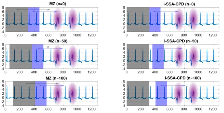
The usefulness of basic SSA is illustrated in the example depicted in Figure1where the wandering baseline 156

of an ECG signal (blue solid line) is removed by subtracting the trend reconstructed through SSA (with a window 157

length ofM=100 and using the first two eigentripleseXI=eXi1+eXi2 −→X˜N= (x˜1,. . .,x˜N)(red solid line))

158

from the original signal, i.e. 159

XNcleaned =XN−XeN= (x1,. . .,xN)−

˜

xi11,. . .,x˜i1N

−x˜i21,. . .,x˜i2N

(7)

yielding the cleaned ECG signal (green solid line). 160

0 200 400 600 800 1000 1200

samples

-200 -100 0 100 200 300

ECG signal

Trend approx. by leading 2 eigentriples

0 200 400 600 800 1000 1200

samples

-200 -100 0 100

200 ECG signal (baseline wander removed)

Figure 1.Application example of basic SSA: baseline wander removal. Showing excerpt 02:20 - 02:30 from record 14149m MIT-BIH ltdb [46]

For a more detailed discussion of SSA, we refer to two well-known monographs [37,48] in the field as well 161

as [44,47] and references therein. 162

2.2. SSA Based Change Detection: Prior Art 163

The sequential application of SSA described in the following is based on work by Moskvina and Zhigljavsky 164

and will be referred to as MZ in the remainder of this paper (see[35–37]). The need for an adaptation of basic

165

SSA is due to the circumstance that it operates in batch mode and is therefore not suited for online change-point 166

detection. 167

Assume a truly sequential problem in which observationsx1,x2,. . . arrive one at a time. Having collected a

168

sufficiently large numberNof observations, MZ constructs the trajectory matrixX(_Bn)(the subindex B refers to

169

‘base’ for reasons that will become obvious in a moment) for time indexnwithM≤N/2,K=N−M+1 and

170

performs the SVD and grouping steps as in basic SSA yielding anl-dimensional subspaceL(n)

I ⊂R

M_spanned

171

by the respective eigenvectors which captures the main structure of the signal. 172

The basic idea of MZ relies on the fact that the distance between the vectorsX(_jn),j=1,. . .,KandL(n)

I , 173

controlled by the specific choice ofI, can be reduced to rather small values. If monitoring of the series{xt}N_t=1

174

continues fort>Nwithout a change in the underlying data generating mechanism, the vectorsXj,j>Kare

175

expected to remain relatively close toL(n)

I while, on the other hand, if such a change were to occur at timeN+τ,

176

the distance betweenXj,j≥K+τandLIwould increase as it would move such vectorsXjout of the subspace

177

L(n)

I (see[36] at 2). Therefore, said distance can be used as a test statistic for change-point detection. Note that

178

only the first three steps of basic SSA need to be performed since reconstruction of the original series is not 179

MZ constructs two matrices, the above mentionedbase matrixX(_Bn), i.e. the trajectory matrix using data 181

samples xn+1,. . .,xn+N, and atest matrix X( n)

T using observations xn+p+1,. . .,xn+q+M−1. The former is

182

subjected to SVD and used to obtain the subspaceL(n)

I while the latter serves to calculate the sum of squared

183

Euclidean distances between its column vectors andL(n)

I . This process can be thought of as having two (possibly

184

intersecting) windows (ofM-dimensional data), of lengthKandQ=q−prespectively, slide over the data.

185

186

Let N,M,l,p,q be fixed integers s.t. l < M < N/2 and 0 ≤ p < q. Then, for each n = 0, 1,. . . MZ

187

proceeds as follows: 188

1. Apply SSA on the interval[n+1,n+N]to getL(n)

I 189

(a) Construct the trajectory/base matrixX(_Bn)

190

X(_Bn)=

                  

xn+1 xn+2 . . . xn+K xn+2 xn+3 . . . xn+K+1

..

. ... . .. ...

xn+M xn+M+1 . . . xn+N                    (8)

whereK=N−M+1.

191

192

(b) Singular Value Decomposition ofX(_Bn).

193

194

(c) Selection ofI={i1,. . .,il},l<d ≤Mwithd=max(i, such thatλi>0). 195

196

2. Construct test matrixX(_Tn)on the interval[n+p+1,n+q+M−1]

197

X(_Tn)=

                  

xn+p+1 xn+p+2 . . . xn+q xn+p+2 xn+p+3 . . . xn+q+1

..

. ... . .. ...

xn+p+M xn+p+M+1 . . . xn+q+M−1

                   (9)

3. Compute the detection statisticDn,I,p,q

198

Dn,I,p,q= q X

j=p+1

" X(_jn)

T X(_jn)−

X(_jn)

T U(_In)

U(_In)

T X(_jn)

#

(10)

where X(_jn) = [xn+j,. . .,xn+j+M−1]T andU(_In) =

U_i(n)

1 ,. . .,U (n)

il

is theM×lmatrix of eigenvectors

199

spanningL(n)

I , i.e. Dn,I,p,qis the sum of squared Euclidean distances between the columns ofX

(n)

T and 200

L(n)

I . MZ normalizes the sum of distancesDn,I,p,qto the number of elements inX

(n)

T 201

˜

Dn,I,p,q= Dn,I,p,q

MQ (11)

and further normalizes the test statistic as 202

Sn,I,p,q= ˜ Dn,I,p,q

vn

(12)

such that it does not depend on the unknown variance of the noise (see[35] at 28) with vn being an

203

estimator ofD˜n,I,p,q, e.g.vn=D˜m,I,0,Kwithm≤nsuch that the hypothesis of no change can be accepted. 204

4. Monitoring ofSn,I,p,qusing CUSUM-type Control Charts 206

MZ then constructs the following CUSUM-type control chart 207

W1=S1,I,p,q, Wn+1=max(0,Wn+Sn+1,I,p,q−Sn,I,p,q−κ), n≥1 (13)

withκsuggested asκ=1/3√MQ(see[35] at 29) and thresholdhMZ =1+1.9

√

M(see[35] at 35). A

208

change-point atnis then declared if

209

Wn≥hMV (14)

holds. 210

3. The Proposed Method (l-SSA-CPD) 211

While MZ provides a powerful methodology that could be applied directly to raw ECG (or PPG) data, it 212

exhibits some drawbacks (for the particular application at hand) that motivated the development of the novel 213

approach to be presented below which we shall refer to aslightweight-SSA-ChangePointDetection(l-SSA-CPD).

214

3.1. Motivation and Informal Description of the Improvements 215

As discussed in the preceding Section, MZ makes use of two (possibly intersecting) windows that are slid 216

over the observed time series, one comprising the data that is embedded to form the trajectory matrix, which 217

is then decomposed by means of SVD to identify an appropriate low(er)-dimensional subspace, and another 218

one containing new (or, in case of overlap, a combination of old and new) observations whose distance to said 219

low-dimensional subspace is then used as a test statistic. This entails the quite burdensome step of performing a 220

SVD every time a new data sample becomes available. 221

222

We shall first highlight the main improvements of our method prior to its formal description. 223

• Low Computational Complexity

224

Small variations over time are intrinsic to cardiac signals and may, besides noise and motion artifacts, e.g. 225

be due toHeart Rate Variability. Contrary to anomalies caused by abnormal cardiac excitation phenomena,

226

these changes in the time between consecutive R-peaks are subtle and often not readily discernible. Most 227

importantly, they do not induce changes as severe as to change the signal’s main characteristics which are 228

captured through the decomposition and grouping stages of SSA. This is illustrated in Figure2which shows

229

a raw (unfiltered) ECG signal with two distinctly shaped PVCs (highlighted in purple) in the third quarter 230

of the excerpt. 231

For the task at hand, performing the SVD of a newly generated trajectory matrix each time a new data point 232

becomes available is not strictly necessary. We are able to drastically reduce the computational burden 233

by generating only one initial trajectory matrixX(_B0)and relying on the obtained reference subspaceL(0)

I 234

throughout the monitoring. This is shown in Figure2with the section of the signal highlighted through gray

235

and blue backgrounds representing the intervals used to generateX(_Bn)andX_T(n), respectively. Note how in

236

MZ (left part of Figure2) bothX(_Bn)andX(_Tn)are being slid over the observations while in our algorithm

237

(right part of Figure2) onlyX(_Tn)is a sliding window sinceX_B(n)|∀n=X(

0)

B . 238

• Simplicity

239

By sliding only a single instead of two windows over the time series the entire procedure is simplified and 240

benefits from a reduction in tuning parameters. 241

In fact, while the total numberQof columns inXT is of course relevant, pandqare not since, due to

242

X(_Bn)|∀n=X_B(0)an overlap ofXBandXT can only occur in the firstN−psamples forp<N. While our

243

algorithm allows for such an initial overlap ofXBandXT, the following discussion is purposely limited

244

0 200 400 600 800 1000 1200 -4

-2 0 2 4 6

8 MZ (n=0)

0 200 400 600 800 1000 1200

-4 -2 0 2 4 6

8 l-SSA-CPD (n=0)

0 200 400 600 800 1000 1200

-4 -2 0 2 4 6

8 MZ (n=50)

0 200 400 600 800 1000 1200

-4 -2 0 2 4 6

8 l-SSA-CPD (n=50)

0 200 400 600 800 1000 1200

-4 -2 0 2 4 6

8 MZ (n=100)

0 200 400 600 800 1000 1200

-4 -2 0 2 4 6

8 l-SSA-CPD (n=100)

Figure 2.Comparison of MZ (left) and l-SSA-CPD (right). The computational burden of l-SSA-CPD is greatly reduced compared to MZ by relying on the reference subspace obtained from an initial, non-sliding trajectory matrix (illustrated by the gray background area). Furthermore, note that l-SSA-CPD’s reference subspace remains locked on the main signal’s characteristics while in MZ, since the reference subspace is updated at each observation (illustrated by the gray area sliding as well), it will lock on the two anomalies (highlighted in pink) for some time as the two moving windows are pass over them.

p=N,q=N+1 and accordinglyQ=1 is a very reasonable choice if minimizing the detection delay is

246

of importance, sinceQ>1 entails a smoother behavior of the test statistic and thus a loss of agility (see,

247

e.g.[35] at 30).

248

The question as to whether or notXBandXT should overlap and if so by how much is therefore removed.

249

Furthermore, sincep=N,q=N+1 can generally be recommended (seeSection4), we can omit both

250

tuning parameterspandq.

251

252

• Augmentation of Test Statistic by considering the angle betweenL(0)

I andX

(n)

j 253

Some authors [49–51] successfully proposed a modified version of MZ, wherein the test statistic is based on 254

angles rather than on Euclidean distances. While both approaches are viable on their own merits, we chose 255

to merge them as they augment each other yielding a test statistic that, according to our results on raw ECG 256

and PPG records, performs favorably compared to the test statistic constructed using either one on its own. 257

In other words, we augment and improve upon the test statistic of MZ by making use of the information 258

from the angles betweenL(0)

I andX

(n)

j as well.

259

260

• Improved thresholding through Sequential Ranks CUSUM

261

MZ provides further potential for improvement by employing a CUSUM-type control chart (seeEq. (13-14))

262

whose control limit (or threshold)his obtained through suitable normal approximation and asymptotic

263

considerations (see[35] at 31;see also[36] at 8). The nuisance of having to properly normalize the test

264

statistic (seeEq. (12)) is a direct consequence of this design choice.

265

We instead propose the use of McDonald’s Sequential Ranks CUSUM (SRC) [52] which we deem to be 266

more appropriate and in line with the model-free nature of SSA. 267

268

• Restarting of SRC control chart after it signaled

Lastly, to allow for the detection of multiple and potentially nearby change-points we restart the SRC every 270

time after it signaled an anomaly by exceeding the preset thresholdhSRC.

271

0 1000 2000 3000 4000 5000 6000 7000

-0.5 0 0.5 1

ECG signal (excerpt record 14046m ltdb)

raw ECG

0 1000 2000 3000 4000 5000 6000 7000

0 0.5 1

SRC without restarting

Q=1 Q=20 Q=40 h

SRC

0 1000 2000 3000 4000 5000 6000 7000

0 0.5 1

SRC with restarting

Q=1 Q=20 Q=40 h

SRC

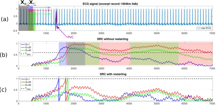
Figure 3.Restarting the SRC each time the threshold was hit (c) is indicated to avoid potentially lengthy delays before the anomaly propagates through and clearsXT(b)

This is indicated since otherwise, depending on the extent of the anomaly (in terms of number of samples) 272

and how it relates to the embedding dimensionMas well as the numberQof columns in the Hankel matrix

273

XT, it may take some time before the anomaly propagates through and clearsXT (i.e. our sliding window)

274

thereby resulting in a return of the test statistic to its ‘baseline level’. This is illustrated in Figure3where,

275

as depicted in (a), three windows (differing in size) withQ={1, 20, 40}are slid over an ECG containing

276

a single PVC (highlighted in purple and marked with an arrow). As can be seen in (b), whileQ=1 is

277

a feasible choice even without restarting the control chart after exceeding the thresholdhSRC, since the

278

respective SRC returns to values belowhSRCafter a relatively long but perhaps still acceptable amount of

279

time, the same cannot be said forQ={20, 40}. Part (c) of Figure3illustrates the clear benefits of restarting

280

the control charts, in that regardless of the choice ofQthe PVC is detected and monitoring for further

281

changes can swiftly resume. As was to be expected,Q=1 is favorable in terms of detection delay.

282

3.2. Formal Description of l-SSA-CPD 283

To allow for better comparison, we use the notation introduced in Section2.2as far as possible.

284

LetN,M,l,p,qbe fixed integers s.t.l<M<N/2 and 0≤p<q. Then our method proceeds as follows:

285

1. Initialization atn=0

286

287

SSA is applied on the interval[n+1,n+N]to getL_I=L(n=0)

I , which akin to MZ involves

288

(a) Construction of the trajectory/base matrixXB=X(

0)

B =X

(n=0)

B .

289

XB=                   

xn+1 xn+2 . . . xn+K xn+2 xn+3 . . . xn+K+1

..

. ... . .. ...

xn+M xn+M+1 . . . xn+N                   

(15)

whereK=N−M+1.

290

(b) Singular Value Decomposition ofXB. 292

293

(c) Selection ofI={i1,. . .,il},l<d ≤Mwithd=max(i, such thatλi>0). 294

295

Then, for eachn=0, 1,. . . we proceed as follows

296

297

2. Construct test matrixX(_Tn)on the interval[n+p+1,n+q+M−1]

298

X_T(n)=X(_j|n)

j=p+1,...,q

=                   

xn+p+1 xn+p+2 . . . xn+q xn+p+2 xn+p+3 . . . xn+q+1

..

. ... . .. ...

xn+p+M xn+p+M+1 . . . xn+q+M−1

                   (16)

withX(_jn)= [xn+j,. . .,xn+j+M−1]T.

299

300

3. Compute the detection statisticsD†_n1,_,I..._,p,3_,q 301

D†1

n,I,p,q= 1 Q

q X

j=p+1

" X(_jn)

T X(_jn)−

X(_jn)

T

UI(UI)TX( n)

j #

(17)

D†2

n,I,p,q=1−cos

∠

X(_Tn),L_I

(18)

D†3

n,I,p,q=D

†₁

n,I,p,q◦D

†₂

n,I,p,q (19)

with 302

∠

X(_Tn),L_I

=∠

X(_Tn),UI

= 1

Q q X

j=p+1

1 l            il X

k=i1

arccos           

hX(_jn),Uki

X

(n)

j kUkk

                      (20)

taking values inh0,π₂i, accordingly D†2

n,I,p,q ∈ [0, 1], UI = [Ui1,. . .,Uil] being the M×l matrix of

303

eigenvectors spanningLI, and◦denoting the Hadamard (element-wise) product.

304

305

4. Monitoring ofD†_n1,_,I..._,p,3_,qusing the Sequential Ranks CUSUM Control Chart

306

Let us denote the sequential rank ofD†_n1,_,I..._,p,3_,qas 307

Rn=1+ n−1

X

r=1

max

0,D†_n1,_,I..._,p,3_,q−D†_r,1,_I..._,p,3_,q

(21)

The Sequential Ranks CUSUM is then 308

Cn=max

0,Cn−1+

Rn

n+1−kSRC

, n≥1 (22)

withC0=0 andkSRCbeing a reference constant.

309

The SRC then signals and a change-point atnis declared if

310

holds, i.e. ifCnexceeds a predetermined control limithSRC.

311

It can be shown [52] that, given that no change in the monitored signal occurred, the quantities Rn

n+1are

312

independent and discrete uniform on 313

{ 1

n+1, 2 n+1,· · · ,

n n+1}

which represents a crucial advantage of the SRC in that it implies that for anykSRCwe can obtain the control

314

limithSRCwithout the need for any historical training data or further assumptions through simulations as

315

follows: 316

Algorithm 1:CalculatehSRCfor fixedkSRC

(a) Set a constantNSRC

(b) fori=1toBdo

i. Construct the set of random variables{Yn}_nN₌SRC₁ as discrete uniform on{_n+1₁,_n+2₁,· · · ,_n+n₁}

ii. ConstructCSRCn =max{0,CSRCn−1+Yn−kSRC}

iii. Extract the maximum value of{CSRCn}

NSRC

n=1

end

(c) Set the control limithSRCas theB·(1−ARL0−1)ordered extracted maximum value withARL0being

the nominal in-control average run length (ARL) (seeAppendixA).

4. Performance Evaluation 317

To evaluate and assess the performance and utility of our method we use records which are publicly 318

available through Physiobank [46], a vast and commonly used resource for ECG and other biophysiological 319

data. In particular, since we claim our method to be suitable for both ECG and PPG data, we found the 320

Physionet Challenge 2015 training database (PC15) [45] to be of particular interest as it provides a collection 321

of synchronized ECG and PPG recordings from which we chose a subset similar to the one used in [53]. With 322

PC15 records not being annotated, we purposely chose to limit our evaluation to records containing PVCs (with 323

different frequencies of occurrence) since they can quite accurately be spotted by careful visual inspection.

324

Before presenting some results, it seems appropriate to briefly restate the goal of our method, which is 325

to provide a lightweight, model-free tool capable of providing a rough assessment under tight constraints on 326

computational resources, e.g. as a pre-screening tool. It is therefore not to substitute for but rather to complement 327

more sophisticated and (computationally) expensive procedures. 328

4.1. Performance Metrics 329

In reporting our results we rely on established metrics commonly used in the literature and reportsensitivity

330

(Se),specificity(Sp), andaccuracy(Acc) defined as

331

S e= T P

T P+FN (24)

S p= T N

T N+FP (25)

Acc= T P+T N

T P+FP+FN+T N (26)

withT P,FP,T N,FNbeing the number oftrue positives,false positives,true negatives, andfalse negatives,

332

Accordingly,sensitivityquantifies the ability to correctly detect actual anomalies while vice versaspecificity 334

quantifies the proportion of non-abnormal segments that are correctly identified as such.Accuracy, on the other

335

hand, assesses the overall performance in terms of both correctly identified abnormal and non-abnormal segments. 336

337

Note that there is a nonzero detection delay introduced by the use of a control chart. Typically, said

338

delay tends to be longer for nonparametric control charts such as the SRC compared to parametric charts (see, 339

e.g.[52]). Use of the latter however would require imposing a parametric model and therefore inevitably conflict

340

with our goal of minimizing (distributional) assumptions as much as possible. 341

For an event occurring at time instancenwe allow for a certain detection delayτdand consider a signal

342

from the control chart as true positive if it falls in the interval[n,n+τd]. All results presented here were obtained

343

usingτd=N, i.e. we allow for a detection delay less or equal to the length of the interval used to construct the

344

initial trajectory matrixXB.

345

Furthermore, note that when directly comparing (synchronized) ECG and PPG signals there is an inherent 346

delay (between the R-peak of the ECG and the respective pulse peak in the PPG) in the PPG signal due to 347

the propagation delay of the pulse pressure wave through the arterial system. This is commonly referred to as 348

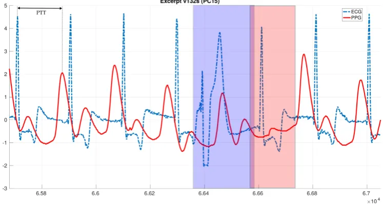
Pulse Arrival Time(PAT) orPulse Transit Time(PTT) (see, e.g.[9,54]) and illustrated on a short data excerpt 349

(containing a single PVC, highlighted by blue and red backgrounds for ECG and PPG, respectively) in Figure4.

350

To account for the PTT delay, when dealing with PPG signals we shift the interval[n,n+τd]byb2M/5c, taken

351

to be a rough estimate of the actual PTT. 352

6.58 6.6 6.62 6.64 6.66 6.68 6.7

104

-3 -2 -1 0 1 2 3 4

5 Excerpt v132s (PC15)

ECG

PPG

Figure 4.Excerpt of a synchronized recording of ECG (blue dash-dotted) and PPG (red solid) containing a single ectopic beat, highlighted with blue and red backgrounds respectively. Note the shift between the R-peak of the ECG and the respective pulse peak of the PPG, known as Pulse Transit Time (PTT)

4.2. Setup and l-SSA-CPD Parameters 353

The PC15 database [45] provides a collection of ECG and PPG recordings from which we chose a subset 354

similar to the one used in [53]. With PC15 records not being annotated, we purposely chose to limit our evaluation 355

to records containing PVCs (with different frequencies of occurrence), since they can quite accurately be spotted

356

by careful visual inspection, eventually including 8 records (composed of two ECG and one PPG signal per 357

record) with varying frequency of PVC occurrence in our analysis. The records are approximately 5 minutes 358

long with the sampling frequency being 250Hz yielding about 75000 observations each. 359

Since an in-depth discussion of how to select important SSA tuning parameters, most notably window 360

lengthMand number of eigentriples used (i.e. selection ofI), would be beyond the scope of this paper (see, e.g.

[35–37,44,47,48] and references therein), it shall suffice to briefly discuss our settings and the rationale behind 362

them. 363

Consider a periodic signal with periodT, then for SSA to capture the main structure of the signal it is

364

important thatMbe at least equal toT. Taking into account the physiological limits on HR and the sampling

365

frequency of our signals,M=300 appears to be a safe and reasonable choice. Accordingly, since as discussed

366

in Section2.1.1we imposeM ≤N/2, we setN = 2M =600. Furthermore, we setIto contain the leading

367

l eigentriples such as to account for 90% of the data’s variance. As for the SRC’s control limit, we use

368

hSRC =79.4107 which we obtained through Algorithm1forB=106,NSRC =5000,ARL0=5000,kSRC =0.5.

369

370

It shall further be emphasized that we apply l-SSA-CPD on the raw unfiltered data without any preprocessing 371

steps. Clearly, suitable preprocessing steps might further enhance performance, the objective here however is to 372

ascertain whether or not usable pre-screening information (pertaining to presence or absence of anomalies) can 373

be obtained by solely applying our l-SSA-CPD with very general parameter settings. A direct performance 374

comparison to MZ is therefore omitted for two main reasons: 375

• MZ would be computationally prohibitively expensive.

376

Recall that the PC15 records are approximately 75·103samples long, requiring computing the SVD of a

377

300×301 trajectory matrix, assumingM=300,N=600,K=N−M+1,Q=1 about 74100 times as

378

opposed to just once for l-SSA-CPD (seeFigure2).

379

• We aim to assess whether, based on its own merits, the performance of l-SSA-CPD suffices to be considered

380

for potential real life applications such as the use case presented in this paper. To further this goal an 381

in-depth comparative analysis to competing algorithms is not required and deemed to be beyond the scope 382

of this paper. 383

4.3. Performance Evaluation Using ECG Signals 384

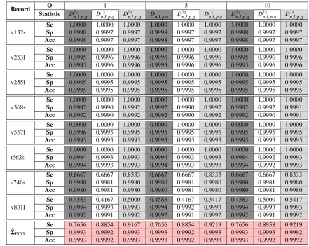
Table1shows the experimental results obtained by applying l-SSA-CP configured as described above to 8

385

PC15 ECG records with varying lengthQ={1, 5, 10}of the test matrixX(_Tn).

386

A crucial condition for l-SSA-CPD to work properly is that the firstNsamples, which are embedded to

387

form the trajectory matrixXB, be an adequate representation of the underlying signal. In other words, we require

388

this initial segment to be free of anomalies. If an anomaly occurs in the firstNsamples, those samples are to

389

be discarded. This was the case for record t662s, which contains a premature ventricular contraction at about 390

n=332<Nand required us to discard the first few hundred observations.

391

Examining the entries of Table1it is apparent that l-SSA-CPD performs well, especially keeping in mind

392

that in our setup it is applied with fairly general parameters to raw, unfiltered ECG traces. The bottom of the 393

table highlighted in red presents the average performance over the entire 8 records for the three different test

394

statistics{D†1

n,I,p,q,D

†₂

n,I,p,q,D

†₃

n,I,p,q}and test matrix widthsQ={1, 5, 10}. 395

Note the increased performance of l-SSA-CPD with test statisticD†3

n,I,p,qand the rather small benefit (if 396

any) of using larger values forQ. These findings corroborate our recommendations made in Section3.1to use

397 D†3

n,I,p,qandQ=1, with the latter being in agreement with results reported by other authors (see, e.g.[35,36]).

398

Table 1.Detection on PC15 ECG trace I

Record Q 1 5 10

Statistic D†1

n,I,p,q D

†2

n,I,p,q D

†3

n,I,p,q D

†1

n,I,p,q D

†2

n,I,p,q D

†3

n,I,p,q D

†1

n,I,p,q D

†2

n,I,p,q D

†3

n,I,p,q

v132s

Se 1.0000 1.0000 1.0000 1.0000 1.0000 1.0000 1.0000 1.0000 1.0000

Sp 0.9998 0.9997 0.9997 0.9998 0.9997 0.9997 0.9998 0.9997 0.9997

Acc 0.9998 0.9997 0.9997 0.9998 0.9997 0.9997 0.9998 0.9997 0.9997

v253l

Se 1.0000 1.0000 1.0000 1.0000 1.0000 1.0000 1.0000 1.0000 1.0000

Sp 0.9995 0.9996 0.9996 0.9995 0.9996 0.9996 0.9995 0.9996 0.9996

Acc 0.9995 0.9996 0.9996 0.9995 0.9996 0.9996 0.9995 0.9996 0.9996

v255l

Se 1.0000 1.0000 1.0000 1.0000 1.0000 1.0000 1.0000 1.0000 1.0000

Sp 0.9995 0.9995 0.9995 0.9995 0.9995 0.9995 0.9995 0.9995 0.9995

Acc 0.9995 0.9995 0.9995 0.9995 0.9995 0.9995 0.9995 0.9995 0.9995

v368s

Se 1.0000 1.0000 1.0000 1.0000 1.0000 1.0000 1.0000 1.0000 1.0000

Sp 0.9992 0.9990 0.9992 0.9992 0.9990 0.9992 0.9992 0.9992 0.9991

Acc 0.9992 0.9990 0.9992 0.9992 0.9990 0.9992 0.9992 0.9990 0.9991

v557l

Se 0.0000 1.0000 1.0000 0.0000 1.0000 1.0000 0.0000 1.0000 1.0000

Sp 0.9996 0.9995 0.9995 0.9995 0.9995 0.9995 0.9995 0.9995 0.9995

Acc 0.9995 0.9995 0.9995 0.9995 0.9995 0.9995 0.9995 0.9995 0.9995

t662s

Se 1.0000 1.0000 1.0000 1.0000 1.0000 1.0000 1.0000 1.0000 1.0000

Sp 0.9994 0.9993 0.9993 0.9994 0.9993 0.9993 0.9994 0.9992 0.9993

Acc 0.9994 0.9993 0.9993 0.9994 0.9993 0.9993 0.9994 0.9992 0.9993

a746s

Se 0.6667 0.6667 0.8333 0.6667 0.6667 0.8333 0.6667 0.6667 0.8333

Sp 0.9980 0.9981 0.9980 0.9980 0.9981 0.9980 0.9980 0.9981 0.9980

Acc 0.9980 0.9981 0.9980 0.9980 0.9981 0.9980 0.9980 0.9981 0.9980

v831l

Se 0.4583 0.4167 0.5000 0.4583 0.4167 0.5417 0.4583 0.5000 0.5417

Sp 0.9994 0.9993 0.9993 0.9994 0.9992 0.9993 0.9994 0.9993 0.9993

Acc 0.9992 0.9991 0.9992 0.9992 0.9991 0.9992 0.9992 0.9991 0.9992

¯ ΣECG

Se 0.7656 0.8854 0.9167 0.7656 0.8854 0.9219 0.7656 0.8958 0.9219

Sp 0.9993 0.9992 0.9993 0.9993 0.9992 0.9993 0.9993 0.9993 0.9992

Acc 0.9993 0.9992 0.9993 0.9993 0.9992 0.9993 0.9993 0.9992 0.9992

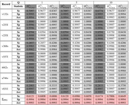
4.4. Performance Evaluation Using PPG Signals 400

Experimental results obtained by applying l-SSA-CPD to the PPG trace of the same 8 PC15 records are 401

shown in Table2, again with varying lengthQ={1, 5, 10}of the test matrixX(_Tn).

402

Comparing the entries of Table2with those Table1we notice an overall drop in performance. Nevertheless,

403

l-SSA-CPD still manages to provide reasonable results. Furthermore, the recommendation of usingD†3

n,I,p,qand 404

Q=1 is shown to hold for the PPG traces as well.

405

406

It should be pointed out that, as has already been observed by other authors (see, e.g. [53]), there are

407

some inconsistencies in the PC15 records in that the some of the supposedly synchronized PPG traces exhibit an 408

unusual delay not consistent with the assumption that the PPG pulse peak should have an offset equal to the

409

PTT with respect to the respective R peak in the ECG. Pflugradt et al. attribute this occasional unusual offset to

410

glitches in the original measurement setup (see[53] at 11) and we assume it to have negatively impacted the

411

performance characteristics presented in Table2since we allow only for a very limited detection delayτd.

Table 2.Detection on PC15 PPG trace

Record Q 1 5 10

Statistic D†1

n,I,p,q D

†2

n,I,p,q D

†3

n,I,p,q D

†1

n,I,p,q D

†2

n,I,p,q D

†3

n,I,p,q D

†1

n,I,p,q D

†2

n,I,p,q D

†3

n,I,p,q

v132s

Se 0.7097 0.9677 0.8387 0.7097 0.9677 0.8387 0.6774 0.9677 0.8387

Sp 0.9995 0.9993 0.9994 0.9995 0.9993 0.9994 0.9995 0.9993 0.9994

Acc 0.9994 0.9993 0.9993 0.9994 0.9993 0.9993 0.9993 0.9993 0.9993

v253l

Se 1.0000 1.0000 1.0000 1.0000 1.0000 1.0000 1.0000 1.0000 1.0000

Sp 0.9996 0.9997 0.9997 0.9996 0.9997 0.9996 0.9996 0.9997 0.9997

Acc 0.9996 0.9997 0.9997 0.9996 0.9997 0.9996 0.9996 0.9997 0.9997

v255l

Se 0.8594 0.8594 0.8438 0.8594 0.8594 0.8438 0.8594 0.8750 0.8438

Sp 0.9999 0.9998 0.9998 0.9999 0.9998 0.9998 0.9999 0.9998 0.9998

Acc 0.9998 0.9997 0.9997 0.9998 0.9997 0.9997 0.9998 0.9997 0.9997

v368s

Se 0.2857 0.2857 0.4286 0.2857 0.4286 0.4286 0.2857 0.4286 0.4286

Sp 0.9983 0.9986 0.9985 0.9983 0.9986 0.9985 0.9983 0.9986 0.9985

Acc 0.9982 0.9986 0.9984 0.9982 0.9986 0.9984 0.9982 0.9986 0.9984

v557l

Se 0.0000 0.0000 0.0000 0.0000 0.0000 0.0000 0.0000 0.0000 0.0000

Sp 0.9997 0.9997 0.9997 0.9997 0.9997 0.9997 0.9997 0.9997 0.9997

Acc 0.9996 0.9996 0.9996 0.9996 0.9996 0.9996 0.9996 0.9996 0.9996

t662s

Se 1.0000 1.0000 1.0000 1.0000 1.0000 1.0000 1.0000 1.0000 1.0000

Sp 0.9988 0.9988 0.9988 0.9988 0.9988 0.9988 0.9988 0.9988 0.9988

Acc 0.9988 0.9988 0.9988 0.9988 0.9988 0.9988 0.9988 0.9988 0.9988

a746s

Se 0.8333 1.0000 1.0000 0.8333 1.0000 1.0000 0.8333 1.0000 0.8333

Sp 0.9995 0.9996 0.9996 0.9995 0.9996 0.9995 0.9995 0.9996 0.9995

Acc 0.9995 0.9996 0.9996 0.9995 0.9996 0.9995 0.9995 0.9996 0.9995

v831l

Se 0.2083 0.3333 0.3333 0.2083 0.3333 0.3750 0.2833 0.3333 0.3750

Sp 0.9997 0.9997 0.9997 0.9997 0.9997 0.9997 0.9997 0.9997 0.9997

Acc 0.9995 0.9995 0.9995 0.9995 0.9995 0.9995 0.9995 0.9995 0.9995

¯ ΣPPG

Se 0.6121 0.6808 0.6806 0.6120 0.6986 0.6858 0.6174 0.7006 0.6649

Sp 0.9994 0.9994 0.9994 0.9994 0.9994 0.9994 0.9994 0.9994 0.9994

Acc 0.9993 0.9994 0.9993 0.9993 0.9994 0.9993 0.9993 0.9994 0.9993

5. Discussion and Outlook 413

In this paper, we have proposed e a novel lightweight and model-free approach for the online detection of 414

cardiac anomalies such as ectopic beats in ECG or PPG signals based on the change detection capabilities of 415

Singular Spectrum Analysis (SSA) and nonparametric rank-based cumulative sum (CUSUM) control charts. 416

The procedure is able to quickly detect anomalies without requiring the identification of fiducial points such as 417

R-peaks and is computationally significantly less demanding than previously proposed SSA-based approaches. 418

This is accomplished by modifying the conventional SSA-based change detection algorithm such that the 419

computationally expensive task of computing the SVD is only performed at the very beginning instead of each 420

time a new data point becomes available. Furthermore, our procedure uses more elaborate test statistics that take 421

into account the information derived from the angle between data vectors representing new observations and the 422

subspace representing the signals characteristics as well as the euclidean distances. Lastly, our procedure differs

423

from previous approaches also in that rank-based control limits and the reinitialization of control charts after an 424

anomaly has been detected are used. 425

Using a set of ECG and PPG records we demonstrated that the direct application of our l-SSA-CPD without 426

any further pre- or post-processing yields not only viable but surprisingly accurate results with an average 427

sensitivity and specificity of 0.9167 and 0.9993 for ECG and 0.6806 and 0.9994 for PPG records, respectively. 428

With regards to the selection and fine-tuning of SSA-parameters, the performance evaluation on records 429

containing cardiac anomalies other than PVCs and a comparative performance analysis, questions for future 430

works are left open. 431

Acknowledgments:The work of M. Lang was supported by the ’Excellence Initiative’ of the German Federal and State

432

Governments and the Graduate School of Excellence Computational Engineering at Technische Universtät Darmstadt. The

views expressed in this article are solely those of the author in his private capacity and do not necessarily reflect the views of

434

Technische Universtät Darmstadt or any other organization.

435

Conflicts of Interest:The author declares no conflict of interest.

436

Abbreviations 437

The following abbreviations are used in this manuscript:

438 439

ANN Artificial Neural Network ARL Average Run Length AV Atrioventricular Node CUSUM Cumulative Sum Control Chart ECG Electrocardiography

HR Heart Rate

PAC Premature Atrial Contraction PAT Pulse Arrival Time

PCA Principal Component Analysis PPG Photoplethysmography

PR Pulse Rate

PTT Pulse Transit Time

PVC Premature Ventricular Contraction SA Sinoatrial Node

SRC Sequential Ranks CUSUM Control Chart SSA Singular Spectrum Analysis

SVD Singular Value Decomposition

440

Appendix A. CUSUM Control Charts 441

Consider an observed sequence {x(n),n ≥ 1} of independent random variables such that

442

{x(1),. . .,x(τ−1)} ∼ F and{x(τ),x(τ+1),. . .} ∼ G, i.e. a distributional shiftF → Goccurs at time 443

instanceτ.

444

Under the assumption thatFandGwere normally distributed with known parameters, Page’s CUSUM [55]

445

represents the gold-standard change detection technique and can be computed sequentially as 446

CC(0) =0, CC(n) =max{0,CC(n−1) +x(n)−kC}, n≥1 (A1) The CUSUM signals, thereby declaring a distributional shift to have occurred, if

447

CC(n)>hC (A2)

with pre-specified control limit/threshold and reference constanthCandkC, respectively. hCandkCare

448

chosen such that a nominal average run length (ARL) of ARL0is attained when the control chart operates

449

in-control, i.e. without distributional shifts occurring (see, e.g.[56]).

450

Formally, the in-control ARL is defined as the expected time until a change is signaled underF, i.e.

451

ARL=EFinf{n>0:CC(n)>hC}. (A3) which can be interpreted as akin to setting a nominal type-I error level in hypothesis testing with the 452

closeness of the actual in-controlARLtoARL0then being an indicator of the CUSUM chart’s robustness [57]. It

453

is well known that, under some regularity conditions, choosingkC=δ/2, withδbeing the shift in the transition

454

F→G, is optimal [58]. 455

References 456

1. Mukhopadhyay, S.C., Ed. Wearable Electronics Sensors - For Safe and Healthy Living, 1st ed.; Springer, 2015.

2. Selke, S., Ed. Lifelogging: Digital self-tracking and Lifelogging - between disruptive technology and cultural

458

transformation, 1st ed.; Springer, 2016.

459

3. Iaizzo, P.A., Ed. Handbook of Cardiac Anatomy, Physiology, and Devices, 3rd ed.; Springer International Publishing,

460

2015.

461

4. Gupta, R.; Mitra, M.; Bera, J. ECG Acquisition and Automated Remote Processing, 1st ed.; Springer, 2014.

462

5. Gacek, A.; Pedrycz, W. ECG Signal Processing, Classification and Interpretation: A Comprehensive Framework of

463

Computational Intelligence, 1st ed.; Springer, 2012.

464

6. Kiasaleh, K. Biological Signals Classification and Analysis, 1st ed.; Springer, 2015.

465

7. Webster, J., Ed. Design of Pulse Oximeters, 1st ed.; CRC Press, 1997.

466

8. Sazonov, E.; Neuman, M.R., Eds. Wearable Sensors: Fundamentals, Implementation and Applications, 1st ed.;

467

Academic Press, 2014.

468

9. Allen, J. Photoplethysmography and its application in clinical physiological measurement. Physiological

469

Measurement2007, 28, R1–R39.

470

10. Adibi, S., Ed. Mobile Health - A Technology Road Map, 1st ed.; Springer International Publishing, 2015.

471

11. Holzinger, A.; Röcker, C.; Ziefle, M., Eds. Smart Health - Open Problems and Future Challenges, 1st ed.; Springer

472

International Publishing, 2015.

473

12. Malvey, D.; Slovensky, D.J. mHealth: Transforming Healthcare, 1st ed.; Springer US, 2014.

474

13. Lang, M. Heart Rate Monitoring Apps: Information for Engineers and Researchers About the New European Medical

475

Devices Regulation 2017/745. JMIR Biomed Eng2017, 2, e2.

476

14. Quinn, P. The EU commission’s risky choice for a non-risk based strategy on assessment of medical devices.

477

Computer Law & Security Review2017, 33, 361–370.

478

15. Sperlich, B.; Holmberg, H.C. Wearable, yes, but able. . . ?: it is time for evidence-based marketing claims! Br J Sports

479

Med Published Online First: 16 December 2016, doi: 10.1136/bjsports-2016-097295.

480

16. Lang, M. Beyond Fitbit: A Critical Appraisal of Optical Heart Rate Monitoring Wearables and Apps, their Current

481

Limitations and Legal Implications. Alb. L. J. Sci. & Tech.2018, 28. forthcoming.

482

17. Tripathi, O.N.; Ravens, U.; Sanguinetti, M.C., Eds. Heart Rate and Rhythm: Molecular Basis, Pharmacological

483

Modulation and Clinical Implications, 1st ed.; Springer Berlin Heidelberg, 2011.

484

18. Jangra, M.; Dhull, S.K.; Singh, K.K., Recent trends in arrhythmia beat detection: A review. In Communication and

485

Computing Systems; Prasad, B.; Singh, K.K.; Ruhil, N.; Singh, K.; O’Kennedy, R., Eds.; Taylor & Francis Group,

486

CRC Press, 2016; pp. 177–183.

487

19. Veeravalli, B.; Deepu, C.J.; Ngo, D., Real-Time, Personalized Anomaly Detection in Streaming Data for Wearable

488

Healthcare Devices. In Handbook of Large-Scale Distributed Computing in Smart Healthcare; Khan, S.U.; Zomaya,

489

A.Y.; Abbas, A., Eds.; Springer International Publishing, 2017; pp. 403–426.

490

20. Elgendi, M.; Eskofier, B.; Dokos, S.; Abbott, D. Revisiting QRS Detection Methodologies for Portable, Wearable,

491

Battery-Operated, and Wireless ECG Systems. PLOS ONE2014, 9, 1–18.

492

21. Lemkaddem, A.; Proença, M.; Delgado-Gonzalo, R.; Renevey, P.; Oei, I.; Montano, G.; Martinez-Heras, J.A.; Donati,

493

A.; Bertschi, M.; Lemay, M. An autonomous medical monitoring system: Validation on arrhythmia detection. 2017

494

39th Annual International Conference of the IEEE Engineering in Medicine and Biology Society (EMBC), 2017, pp.

495

4553–4556.

496

22. Ye, C.; Coimbra, M.T.; Kumar, B.V.K.V. Arrhythmia detection and classification using morphological and dynamic

497

features of ECG signals. 2010 Annual International Conference of the IEEE Engineering in Medicine and Biology,

498

2010, pp. 1918–1921.

499

23. Chang, R.C.H.; Lin, C.H.; Wei, M.F.; Lin, K.H.; Chen, S.R. High-precision real-time premature ventricular contraction

500

(PVC) detection system based on wavelet transform. Journal of Signal Processing Systems2014, 77, 289–296.

501

24. Yaghouby, F.; Ayatollahi, A.; Bahramali, R.; Yaghouby, M.; Alavi, A. Towards automatic detection of atrial fibrillation:

502

a hybrid computational approach. Comput. Biol. Med.2010, 40, 919–930.

503

25. Acharya, U.; Bhat, B.; Iyengar, S.; Rao, A.; Dua, S. Classification of heart rate data using artificial neural network

504

and fuzzy equivalence relation. Pattern Recognit.2003, 36, 61–68.

505

26. Kumar, S.; Bansal, A.; Tiwari, V.; Nayak, M.; Narayanan, R. Remote health monitoring system for detecting cardiac

506

disorders. Proceedings of 2014 IEEE International Conference on Bioinformatics and Biomedicine, 2014, pp. 30–34.

507

27. Gradl, S.; Kugler, P.; Lohmüller, C.; Eskofier, B. Real-time ECG monitoring and arrhythmia detection using

508

Android-based mobile devices. 2012 Annual International Conference of the IEEE Engineering in Medicine and

509

Biology Society, 2012, pp. 2452–2455.

28. Luz, E.J.S.; Schwartz, W.R.; Cámara-Chávez, G.; Menotti, D. ECG-based heartbeat classification for arrhythmia

511

detection: A survey. Computer Methods and Programs in Biomedicine2016, 127, 144–164.

512

29. Oresko, J.J.; Jin, Z.; Cheng, J.; Huang, S.; Sun, Y.; Duschl, H.; Cheng, A.C. A Wearable Smartphone-Based

513

Platform for Real-Time Cardiovascular Disease Detection Via Electrocardiogram Processing. IEEE Transactions on

514

Information Technology in Biomedicine2010, 14, 734–740.

515

30. Amiri, A.M.; Abhinav.; Mankodiya, K. m-QRS: An efficient QRS detection algorithm for mobile health applications.

516

2015 17th International Conference on E-health Networking, Application Services (HealthCom), 2015, pp. 673–676.

517

31. Kim, Y.J.; Heo, J.; Park, K.S.; Kim, S. Proposition of novel classification approach and features for improved

518

real-time arrhythmia monitoring. Computers in biology and medicine2016, 75, 190–202.

519

32. Tsipouras, M.G.; Fotiadis, D.I. Automatic arrhythmia detection based on time and time–frequency analysis of heart

520

rate variability. Computer Methods and Programs in Biomedicine2004, 74, 95–108.

521

33. de Chazal, P.; O’Dwyer, M.; Reilly, R.B. Automatic classification of heartbeats using ECG morphology and heartbeat

522

interval features. IEEE Transactions on Biomedical Engineering2004, 51, 1196–1206.

523

34. Pan, J.; Tompkins, W.J. A Real-Time QRS Detection Algorithm. IEEE Transactions on Biomedical Engineering

524

1985, BME-32, 230–236.

525

35. Moskvina, V. Application of the Singular Spectrum Analysis for change-point detection in time serie. PhD thesis,

526

UK, 2001. CardiffUniversity.

527

36. Moskvina, V.; Zhigljavsky, A. An Algorithm Based on Singular Spectrum Analysis for Change-Point Detection.

528

Communications in Statistics2003, 32, 319–352.

529

37. Golyandina, N.; Nekrutkin, V.; Zhigljavsky, A. Analysis of Time Series Structure: SSA and related techniques, 1st

530

ed.; Chapman & Hall/CRC Monographs on Statistics & Applied Probability (Book 90), Chapman and Hall/CRC,

531

2001.

532

38. Dong, Q.; Yang, Z.; Chen, Y.; Li, X.; Zeng, K. Anomaly Detection in Cognitive Radio Networks Exploiting Singular

533

Spectrum Analysis. International Conference on Mathematical Methods, Models, and Architectures for Computer

534

Network Security. Springer, 2017, pp. 247–259.

535

39. Yang, Z.; Zhou, N.; Polunchenko, A.; Chen, Y. Singular Spectrum Analysis Based Quick Online Detection of

536

Disturbance Start Time in Power Grid. 2015 IEEE Global Communications Conference (GLOBECOM), 2015, pp.

537

1–6.

538

40. Zhang, S.; Liu, Y.; Pei, D.; Chen, Y.; Qu, X.; Tao, S.; Zang, Z.; Jing, X.; Feng, M. FUNNEL: Assessing Software

539

Changes in Web-based Services. IEEE Transactions on Services Computing2016, PP.

540

41. Georgescu, V.; Delureanu, S.M. Fuzzy-valued and complex-valued time series analysis using multivariate and complex

541

extensions to singular spectrum analysis. 2015 IEEE International Conference on Fuzzy Systems (FUZZ-IEEE),

542

2015, pp. 1–8.

543

42. Jarchi, D.; Lo, B.; Wong, C.; Ieong, E.; Nathwani, D.; Yang, G.Z. Gait Analysis From a Single Ear-Worn

544

Sensor: Reliability and Clinical Evaluation for Orthopaedic Patients. IEEE Transactions on Neural Systems and

545

Rehabilitation Engineering2016, 24, 882–892.

546

43. Uus, A.; Liatsis, P. Singular Spectrum Analysis for detection of abnormalities in periodic biosignals. 2011 18th

547

International Conference on Systems, Signals and Image Processing, 2011, pp. 1–4.

548

44. Sanei, S.; Hassani, H. Singular Spectrum Analysis of Biomedical Signals, 1st ed.; CRC Press, 2016.

549

45. Clifford, G.; Silva, I.; Moody, B.; Li, Q.; Kella, D.; Shahin, A.; Kooistra, T.; Perry, D.; Mark, R. The

550

PhysioNet/Computing in Cardiology Challenge 2015: Reducing False Arrhythmia Alarms in the ICU. Computing in

551

cardiology2015, 42, 273–276.

552

46. Goldberger, A.L.; Amaral, L.A.; Glass, L.; Hausdorff, J.M.; Ivanov, P.C.; Mark, R.G.; Mietus, J.E.; Moody, G.B.;

553

Peng, C.K.; Stanley, H.E. Physiobank, physiotoolkit, and physionet. Circulation2000, 101, e215–e220.

554

47. Golyandina, N.; Zhigljavsky, A. Singular Spectrum Analysis for Time Series, 1st ed.; Springer Briefs in Statistics,

555

Springer, 2013.

556

48. Elsner, J.B.; Tsonis, A.A. Singular Spectrum Analysis: A New Tool in Time Series Analysis; Language of Science,

557

Springer, 1996.

558

49. Idé, T.; Inoue, K. Knowledge discovery from heterogeneous dynamic systems using change-point correlations.

559

Proceedings of the 2005 SIAM International Conference on Data Mining. SIAM, 2005, pp. 571–575.

560

50. Mohammad, Y.; Nishida, T. Robust Singular Spectrum Transform. Next-Generation Applied Intelligence: 22nd

561

International Conference on Industrial, Engineering and Other Applications of Applied Intelligent Systems, IEA/AIE

2009, Tainan, Taiwan, June 24-27, 2009. Proceedings; Chien, B.C.; Hong, T.P.; Chen, S.M.; Ali, M., Eds.; Springer

563

Berlin Heidelberg: Berlin, Heidelberg, 2009; pp. 123–132.

564

51. Idé, T.; Tsuda, K. Change-Point Detection using Krylov Subspace Learning. Proceedings

565

of the 2007 SIAM International Conference on Data Mining, 2007, pp. 515–520,

566

[http://epubs.siam.org/doi/pdf/10.1137/1.9781611972771.54].

567

52. McDonald, D.R. A Cusum Procedure Based on Sequential Ranks; Laboratory for Research in Statistics and

568

Probability, Carleton University, 1985.

569

53. Pflugradt, M.; Geissdoerfer, K.; Goernig, M.; Orglmeister, R. A Fast Multimodal Ectopic Beat Detection Method

570

Applied for Blood Pressure Estimation Based on Pulse Wave Velocity Measurements in Wearable Sensors. Sensors

571

2017, 17.

572

54. Salvi, P. Pulse Waves: How Vascular Hemodynamics Affects Blood Pressure, 1st ed.; Springer, 2012.

573

55. Page, E.S. Continuous Inspection Schemes. Biometrika1954, 41, pp. 100–115.

574

56. Lucas, J.M. The Design and Use of Cumulative Sum Control Schemes. Technometrics1976, pp. 51–59.

575

57. Chatterjee, S.; Qiu, P. Distribution-free cumulative sum control charts using bootstrap-based control limits. Ann.

576

Appl. Stat2009, 3, 349–369.

577

58. Reynolds, M.R. Approximations to the average run length in cumulative sum control charts. Technometrics1975, pp.

578

65–71.