From Inception to Implementation
With Applications to the Falcon Signature Scheme
James Howe1, Thomas Prest1, Thomas Ricosset2, and Mélissa Rossi2,3,4,5
1
PQShield, Oxford, UK
[email protected] [email protected] 2
Thales, Gennevilliers, France
ANSSI, Paris, France
4
École normale supérieure, CNRS, PSL University, Paris, France
5 Inria, Paris, France [email protected]
Abstract Gaussian sampling over the integers is a crucial tool in lattice-based cryptography, but has proven over the recent years to be surprisingly challenging to perform in a generic, efficient and provable secure manner. In this work, we present a modular framework for generating discrete Gaussians with arbitrary center and standard deviation. Our framework is extremely simple, and it is precisely this simplicity that allowed us to make it easy to implement, provably secure, portable, efficient, and provably resistant against timing attacks. Our sampler is a good candidate for any trapdoor sampling and it is actually the one that has been recently implemented in the Falcon signature scheme. Our second contribution aims at systematizing the detection of implementation errors in Gaussian samplers. We provide a statistical testing suite for discrete Gaussians called SAGA(Statistically Acceptable GAussian). In a nutshell, our two contributions take a step towards trustable and robust Gaussian sampling real-world implementations.
Keywords.
Lattice based cryptography, Gaussian Sampling, Isochrony, Statistical verification tools
1
Introduction
Gaussian sampling over the integers is a central building block of lattice-based cryptography, in theory as well as in practice. It is also notoriously difficult to perform efficiently and securely, as il-lustrated by numerous side-channel attacks exploiting BLISS’ Gaussian sampler [9,23,54,61]. For this reason, some schemes limit or proscribe the use of Gaussians [6,40]. However, in some situa-tions, Gaussians are unavoidable. The most prominent example is trapdoor sampling [30,53,45]: performing it with other distributions is an open question, except in limited cases [41] which entail a growth O(√n) toO(n) of the output, resulting in dwindling security levels. Given the countless applications of trapdoor sampling (full-domain hash signatures [30,58], identity-based encryption (or IBE) [30,20], hierarchical IBE [11,1], etc.), it is important to come up with Gaus-sian samplers over the integers which are not only efficient, but also provably secure, resistant to timing attacks, and in general easy to deploy.
– Simplicity and Modularity.At a high level, our framework only requires two ingredients (a base sampler and a rejection sampler) and combines them in a simple and black-box way. Not only does it make the description of our sampler modular (as one can replace any of the ingredients), this simplicity and modularity also infuses all aspects of its analysis.
– Genericity. Our sampler is fully generic as it works with arbitrary center µand standard deviation σ. In addition, it does not incur hidden precomputation costs: given a fixed base sampler of parameter σmax, our framework allows to sample from DZ,σ,µ for any ηϵ(Zn) ≤
σ ≤ σmax. In comparison, [47] implicity requires a different base sampler for each different
value ofσ; this limits its applicability for use cases such as Falcon [58], which has up to2048 differentσ’s, all computed at key generation.
– Efficiency and Portability.Our sampler is instantiated with competitive parameters which make it very efficient in time and memory usage. For σmax = 1.8205 and SHAKE256 used
as PRNG, our sampler uses only 512 bytes of memory and achieved 1,848,428 samples per second on an Intel i7-6500U clocked at 2.5 GHz. Moreover, our sampler can be instantiated in a way that uses only integer operations, making it highly portable.
– Provable Security. A security analysis based on the statistical distance would either pro-vide very weak security guarantees or require to increase the running time by an order of magnitude. We instead rely on the Rényi divergence, a tool which in the recent years has allowed dramatic efficiency gains for lattice-based schemes [3,57]. We carefully selected our parameters as to make them as amenable to a Rényi divergence-based analysis.
– Isochrony. We formally show that our sampler is isochronous: its running time is indepen-dent of the inputs σ, µ and of the output z. Isochrony is weaker than being constant-time, but it nevertheless suffices to argue security against timing attacks. Interestingly, our proof of isochrony relies on techniques and notions that are common in lattice-based cryptography: the smoothing parameter, the Rényi divergence, etc. In particular, the isochrony of our sam-pler is implied by parameters dictated by the current state of the art forblack-box security of lattice-based schemes.
One second contribution stems from a simple observation: implementations of otherwise per-fectly secure schemes have failed in spectacular ways by introducing weaknesses, a common one being randomness failure: this is epitomized by nonce reuses in ECDSA, leading to jailbreaking Sony PS3 consoles1 and exposing Bitcoin wallets [8]. The post-quantum community is aware of this point of failure but does not seem to have converged on a systematic way to mitigate it [51]. Randomness failures have been manually discovered and fixed in implementations of Dilithium [50], Falcon [56,52] and other schemes; the case of Falcon is particularly relevant to us because the sampler implemented was the one described in this document!
Our second contribution is a first step at systematically detecting such failures: we propose a statistical test suite called SAGA for validating discrete Gaussians. This test suite can check univariate samples; we therefore use it to validate our own implementation of our sampler. In addition, our test suite can check multivariate Gaussians as well; this enables validation at a higher level: if the base sampler over the integers is validated, but the output of the high-level scheme does not behave like a multivariate Gaussian even though the theory predicts it should, then this is indicative of an implementation mistake somewhere else in the implementation (or, at the worst case, that the theory is deficient). We illustrate that with a simple example of a (purportedly) deficient implementation of Falcon [58], however it can be used for any other scheme sampling multivariate discrete Gaussians, including but not limited to [45,20,29,5,12]. The test suite is publicly available at: https://github.com/PQShield/SAGA.
2
Related Works
In the recent years, there has been a surge of works related to Gaussian sampling over the inte-gers. Building on convolution techniques from [55], [47] proposed an arbitrary-center Gaussian sampler base, as well as a statistical tool (the max-log distance) to analyse it. [3,57,44] revisited classical techniques with the Rényi divergence. Polynomial-based methods were further studied by [57,65,4]. The use of rounded Gaussians was proposed in [34]. Knuth-Yao’s DDG trees have been considered in [22,35].2 Lazy floating-point precision was studied in [21,18]. We note that techniques dating back to von Neumann [62] allow to generate (continuous) Gaussians elegantly using finite automata [27,2,36]. While these have been considered in the context of lattice-based cryptography [19,17] they are also notoriously hard to make isochronous. Finally, [63] studied previously cited techniques with the goal of minimizing their relative error.
3
Preliminaries
3.1 Gaussians
For σ, µ ∈ R withσ > 0, we call Gaussian function of parameters σ, µ and denote by ρσ,µ the function defined over R asρσ,µ(x) = exp
(
−(x−µ)2
2σ2 )
. Note that whenµ= 0we omit it in index
notation, e.g.ρσ(x) =ρσ,0(x). The parameter σ (resp.µ) is often called the standard deviation
(resp. center) of the Gaussian. In addition, for any countable set S⊊ R we abusively denote by
ρσ,µ(S)the sum ∑
z∈Sρσ,µ(z). When ∑
z∈Sρσ,µ(z)is finite, we denote byDS,σ,µand call Gaussian distribution of parameters σ, µ the distribution over S defined by DS,σ,µ(z) =ρσ,µ(z)/ρσ,µ(S). Here too, whenµ= 0we omit it in index notation, e.g.DS,σ,µ(z) =DS,σ(z). We use the notation
Bp to denote the Bernoulli distribution of parameterp.
3.2 Renyi Divergence
We recall the definition of the Rényi divergence, which we will use massively in our security proofs.
Definition 1 (Rényi Divergence). Let P, Q be two distributions such that Supp(P) ⊆
Supp(Q). For a∈(1,+∞), we define the Rényi divergence of ordera by
Ra(P,Q) =
∑
x∈Supp(P)
P(x)a
Q(x)a−1
1 a−1
.
In addition, we define the Rényi divergence of order +∞ by
R∞(P,Q) = max
x∈Supp(P)
P(x)
Q(x).
The Rényi divergence is not a distance; for example, it is neither symmetric nor does it verify the triangle inequality, which makes it less convenient than the statistical distance. On the other hand, it does verify cryptographically useful properties, incluing a few listed below.
Lemma 2 ([3]). For two distributions P,Q and two families of distributions (Pi)i,(Qi)i, the
Rényi divergence verifies these properties:
– Data processing inequality. For any function f, Ra(f(P), f(Q))≤Ra(P,Q).
– Multiplicativity. Ra( ∏
iPi, ∏
iQi) = ∏
iRa(Pi,Qi).
– Probability preservation.For any event E ⊆Supp(Q) anda∈(1,+∞),
Q(E)≥ P(E)a−a1/Ra(P,Q), (1)
Q(E)≥ P(E)/R∞(P,Q). (2)
The following lemma shows that a bound ofδon the relative error between two distributions implies a boundO(aδ2) on the log of the Rényi divergence (as opposed to a boundO(δ)on the statistical distance).
Lemma 3 (Lemma 3 of [57]).Let P,Qbe two distributions of same support Ω. Suppose that the relative error between P andQ is bounded:∃δ >0 such that PQ −1≤δ over Ω. Then, for a∈(1,+∞):
Ra(P,Q)≤ (
1 + a(a−1)δ
2
2(1−δ)a+1
) 1 a−1
∼
δ→01 + aδ2
2
3.3 Smoothing Parameter
For ϵ > 0, the smoothing parameter ηϵ(Λ) of a lattice Λ is the smallest value σ > 0 such that
ρ 1
σ√2π
(Λ⋆\{0}) ≤ ϵ, where Λ⋆ denotes the dual of Λ. In the literature, some definitions of the smoothing parameter scale our definition by a factor √2π. It is shown in [46] that ηϵ(Zn) ≤
ηϵ+(Zn), where:
ηϵ+(Zn) = 1
π
√ 1 2log
( 2n
( 1 +1
ϵ
))
. (3)
3.4 Isochronous algorithms
We now give a semi-formal definition of isochronous algorithms.
Definition 4. Let A be a (probabilistic or deterministic) algorithm with set of input variables
I, set of output variables O, and letS ⊆ I ∪ O be the set of sensitive variables. We say that A is perfectly isochronous with respect to S if its running time is independent of any variable inS. In addition, we say thatA statistically isochronous with respect to S if there exists a distri-bution D independent of all the variables in S, such that the running time of A is statistically close (for a clearly identified divergence) to D.
We note that we can define a notion of computationally isochronous algorithm. For such an algorithm, it is computationally it hard to recover the sensitive variables even given the distribution of the running time of the algorithm. We can even come up with a contrived example of such an algorithm: let A()select in an isochronous manner anx uniformly in a space of min-entropy ≥ λ, compute y = H(x) and wait a time y before outputting x. One can show that recovering x given the running time of Ais hard if H is a one-way function.
4
The sampler
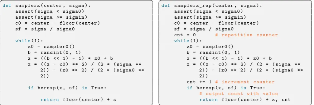
Algorithm 1 SamplerZ(σ, µ)
Require: µ∈[0,1],σ≤σmax Ensure: z∼DZ,σ,µ
1: whileTruedo
2: z0←BaseSampler()
3: b← {0,1}uniformly 4: z:= (2b−1)·z0+b
5: x:= z20
2σ2 max −
(z−µ)2
2σ2
6: if AcceptSample(σ, x)then
7: returnz
Algorithm 2 AcceptSample(σ, x)
Require: σmin≤σ≤σmax, x <0 Ensure: b∼ Bσmin
σ ·exp(x) 1: p:=σmin
σ ·ApproxExp(x) Lazy Bernoulli sampling
2: i:= 1
3: do
4: i:=i·28
5: u←J0,28−1Kuniformly
6: v:=⌊p·i⌋ & 0xff
7: whileu=v 8: return(u < v)
standard deviation as σmax> σmin >0, we present an algorithm that samples the distribution DZ,σ,µ for anyµ∈[0,1]and σmin≤σ≤σmax.
Our sampling algorithm is called SamplerZ and is described in Algorithm1. We denote by BaseSampler an algorithm that samples an element with the fixed half Gaussian distribution
DZ+,σmax. The first step consists in using BaseSampler. The obtained z0 sample is then trans-formed into z := (2b−1)·z0+b where b is a bit drawn uniformly in {0,1}. Let us denote by BGσmax the distribution ofz. The distribution ofzis a discrete bimodal half-Gaussian of centers 0 and 1. More formally,
BGσmax(z) = 1 2
{
DZ+,σmax(−z) ifz≤0
DZ+,σmax(z−1)ifz≥1. (4) Then, to recover the desired distribution DZ,σ,µ for the inputs (σ, µ), one might want to apply the classical rejection sampling technique applied to lattice based schemes [39] and accept
z with probability
DZ,σ,µ(z)
BGσmax(z) = exp ( z2
2σ2 max −
(z−µ)2
2σ2 )
ifz≤0
exp (
(z−1)2
2σ2 max −
(z−µ)2
2σ2 )
ifz≥1
= exp (
z02
2σ2 max
−(z−µ)2
2σ2
)
.
The element inside theexpis computed in step 5. Next, we also introduce an algorithm de-notedAcceptSample. The latter performs the rejection sampling (Algorithm2): usingApproxExp an algorithm that returns exp(·), it returns a Bernoulli sample with the according probability. Actually, for isochrony matters, detailed in Section6, the latter acceptance probability is rescaled by a factor σminσ . As z follows the BGσmax distribution, after the rejection sampling, the final distribution of SamplerZ(σ, µ) is then proportional to σminσ ·DZ,σ,µ which is, after normalization exaclty equal toDZ,σ,µ. Thus, with this construction, one can derive the following proposition.
Proposition 5 (Correctness). Assume that all the uniform distributions are perfect and that BaseSampler=DZ+,σmax andApproxExp= exp, then the construction ofSamplerZ(in Algorithms
1 and2) is such thatSamplerZ(σ, µ) =DZ,σ,µ.
In practical implementations, one cannot acheive perfect distributions. Only acheivingBaseSampler≈
Table 1: Number of calls toSamplerZ,BaseSamplerand ApproxExp
Notation Value forFalcon
Calls to sign (as per NIST) Qs ≤264
Calls toSamplerZ QsamplZ Qs·2·n≤275
Calls toBaseSampler Qbs Niter·QsamplZ≤276
Calls toApproxExp Qexp Qbs≤276
5
Proof of Security
Table1gives the notations for the number of calls toSamplerZ,BaseSamplerandApproxExpand the considered values when the sampler is instanciated forFalcon. Due to the rejection sampling in step 6, there will be a (potentially infinite) number of iterations of the while loop. We will show later in Lemma 7, that the number of iterations follows a geometric law of parameter
≈ σmin·√2π
2·ρσmax(Z+). We noteNiter a heuristic considered maximum number of iterations. By a central limit argument, Niter will only be marginally higher than the expected number of iterations. To
instantiate the values Qexp=Qbs=Niter·QsamplZ for the example of Falcon, we takeNiter = 2.
In fact, σmin·
√ 2π
2·ρσmax(Z+) ≤2 forFalcon’s parameters.
The following Theorem estimates the security of SamplerZ, it is independant of the chosen values for the number of calls.
Theorem 6 (Security of SamplerZ). Let λIdeal (resp. λReal) be the security parameter of an implementation using the perfect distribution DZ,σ,µ (resp. the real distribution SamplerZ).
If both following conditions are respected, at most two bits of security are lost. In other words, ∆λ:=λIdeal−λReal≤2.
∀x <0, ApproxExp(x)−exp(x)
exp(x)
≤
√
2·λReal
2·(2·λReal+ 1)2·Qexp
(Cond. (1))
R2·λReal+1
(
BaseSampler, DZ+,σmax )
≤1 + 1 4·Qbs
(Cond. (2))
The proof of this Theorem is given in AppendixA.
To get concrete numerical values, we assume that256bits are claimed on the original scheme, thus 254bits of security are claimed for the real implementation. Then for an implementation of Falcon, the numerical values are
√
2·λReal
2·(2·λReal+ 1)
2· Qexp
≈2−43 and 1 4·Qbs ≈
2−78.
5.1 Instanciating the ApproxExp
To achieve condition(1)withApproxExp, we use a polynomial approximation of the exponential on[−ln(2),0]. In fact, one can reduce the parameterx moduloln(2)such that x=−r−sln(2). Compute the exponential remains to computeexp(x) = 2−sexp(−r). Noting thats≥64happen very rarely, thusscan be saturated at 63to avoid overflow without loss in precision.
We use the polynomial approximation tool provided in GALACTICS [4]. This tool generates polynomial approximations that allow a computation in fixed precision with chosen size of coefficients and degree. As an example, for 32-bit coefficients and a degree 10, we obtain a polynomial Pgal(x) :=
∑10
◦ a0 = 1;
◦ a1 = 1;
◦ a2 = 2−1;
◦ a3 = 2863311530·2−34;
◦ a4 = 2863311481·2−36;
◦ a5 = 2290647631·2−38;
◦ a6 = 3054141714·2−41;
◦ a7 = 3489252544·2−44;
◦ a8 = 3473028713·2−47;
◦ a9 = 2952269371·2−50;
◦ a10= 3466184740·2−54.
For any x ∈ [−ln(2),0], Pgal verifies
Pgal(x)−exp(x) exp(x)
≤ 2−47, which is sufficient to verify condition (1)for Falconimplementation.
Flexibility on the implementation of the polynomial. Depending on the platform and the requirement for the signature, one can adapt the polynomial to fit their constraints. For example, if one wants to minimize the number of multiplications, implementing the polynomial with Horner’s form is the best option. The polynomial is written in the following form :
Pgal(x) =a0+x(a1+x(a2+x(a3+x(a4+x(a5+x(a6+x(a7+x(a8+x(a9+xa10))))))))).
Evaluating Pgal is then done serially as follows:
y←a10
y←a9+y×x
.. .
y←a1+y×x
y←a0+y×x
Some architectures with small register sizes may be faster if the size of the coefficients of the poly-nomial is minimized, thus GALACTICS tool can be used to generate a polypoly-nomial with smaller coefficients. For example, we propose an alternative polynomial approximation on [0,ln64(2)]with 25 bits coefficients.
P = 1 +x+ 2−1x2+ 699051·2−22·x3+ 699299·2−24·x4+ 605552·2−26·x5
To recover the polynomial approximation on [0, ln(2)], we compute P(64x)64.
Some architectures enjoy some level of parallelism, in which case it is desirable to minimise the depth of the circuit computing the polynomial3. WritingPgal in Estrin’s form [24] is helpful
in this regard.
x2 ←x×x
x4 ←x2×x2
Pgal(x)←(x4×x4)×((a8+a9×x) +x2×a10)
+ (((a0+a1×x) +x2×(a2+a3×x)) +x4×((a4+a5×x) +x2×(a6+a7×x)))
5.2 Instanciating the BaseSampler
Algorithm 3 SampleCDT: full-table access CDT
z←0
u←[0,1)uniformly withθbits of absolute precision
for0≤i≤wdo
b←(CDT[w]≥u) ▷ b= 1if it is true and0otherwise
z←z+b
returnz
of elements of the CDT and the precision of its coefficients. Let a= 2·λReal+ 1. To derive the parameters w andθ we use a simple script that, givenσmax andθ as inputs:
1. Computes the smallest tailcutwsuch that the Renyi divergenceRabetween the ideal distri-butionDZ+,σmaxand its restriction to{0, . . . , w}(notedD[w],σmax) verifiesRa(D[w],σmax, DZ+,σmax)≤ 1 + 1/(4Qbs);
2. Rounds the probability density table (PDT) of D[w],σmax with θ bits of absolute precision. This rounding is done “cleverly” by truncating all the PDT values except the largest:
◦ forz≥1, the value D[w],σmax(z) is truncated: P DT(z) = 2−θ ⌊
2θD[w],σmax(z) ⌋
.
◦ in order to have a probability distribution, P DT(0) = 1−∑z≥1P DT(z).
3. Derives the CDT from the PDT and computes the finalRa(SampleCDTw=19,θ=72, DZ+,σmax). Taking σmax= 1.8205and θ= 72as inputs, we found w= 19.
◦ PDT(0) =2−72×1697680241746640300030
◦ PDT(1) =2−72×1459943456642912959616
◦ PDT(2) =2−72×928488355018011056515
◦ PDT(3) =2−72×436693944817054414619
◦ PDT(4) =2−72×151893140790369201013
◦ PDT(5) =2−72×39071441848292237840
◦ PDT(6) =2−72×7432604049020375675
◦ PDT(7) =2−72×1045641569992574730
◦ PDT(8) =2−72×108788995549429682
◦ PDT(9) =2−72×8370422445201343
◦ PDT(10) =2−72×476288472308334
◦ PDT(11) =2−72×20042553305308
◦ PDT(12) =2−72×623729532807
◦ PDT(13) =2−72×14354889437
◦ PDT(14) =2−72×244322621
◦ PDT(15) =2−72×3075302
◦ PDT(16) =2−72×28626
◦ PDT(17) =2−72×197
◦ PDT(18) =2−72×1
Our experiment showed that for any a ≥ 509, Ra(SampleCDTw=19,θ=72, DZ+,σmax) ≤ 1 + 2−80≤1 +4Q1
bs, which validates condition(2) forFalconimplementation.
6
Analysis of resistance against timing attacks
In this section, we show that Algorithm 1 is impervious against timing attacks. We formally prove that it is isochronous with respect toσ, µ and the outputz (in the sense of Definition 4). We first prove a technical lemma which shows that the number of iterations in the while loop of Algorithm 1is (almost) independent of σ, µ, z.
Lemma 7. Letϵ∈(0,1),µ∈[0,1]and letσmin, σ, σ0 be standard deviations such thatηϵ+(Zn) =
σmin≤σ ≤σ0. Letp= σmin· √
2π
2·ρσmax(Z+). The number of iterations of thewhileloop inSamplerZ(σ, µ)
follows a geometric law of parameter
Ptrue(σ, µ)∈p·
[
1,1 +(1 + 2
−80)ϵ
n
]
.
The proof of Lemma7 can be found in AppendixB.
Next, we show that Algorithm1 is perfectly isochronous with respect to z and statistically isochronous (for the Rényi divergence) with respect to σ, µ.
Theorem 8. Let ϵ ∈ (0,1), µ ∈ R, let σmin, σ, σ0 be standard deviations such that ηϵ+(Zn) =
σmin ≤ σ ≤ σ0, and let p = σmin· √
2π
2·ρσmax(Z+) be a constant in (0,1). Suppose that the elementary
operations {+,−,×, /} over integer and floating-point numbers are isochronous. The running time of Algorithm 1 follows a distributionTσ,µ such that:
Ra(Tσ,µ∥T)≲1 +
aϵ2max(1,1−pp)2
n2(1−p) = 1 +O
(
aϵ2 n2
)
for some distribution T independent of its inputs σ, µ and its output z.
Finally, we leverage Theorem 8 to prove that the running time of SamplerZ(σ, µ) does not help an adversary to break a cryptographic scheme. We consider that the adversary has access to some function g(SamplerZ(σ, µ)) as well as the running time ofSamplerZ(σ, µ): this is intended to capture the fact that in practice the output of SamplerZ(σ, µ) is not given directly to the adversary, but processed by some function before. For example, in the signature scheme Falcon, samples are processed by algorithms depending on the signer’s private key. On the other hand, we consider that the adversary has powerful timing attack capabilities by allowing him to learn the exact runtime of each call to SamplerZ(σ, µ).
Corollary 9. Consider an adversary A making Qs queries to g(SamplerZ(σ, µ)) for some
ran-domized function g, and solving a search problem with success probability 2−λ for some λ≥1. With the notations of Theorem 8, suppose thatmax(1,1−pp)2 ≤n(1−p) andϵ≤ √1
λQs. Learning
the running time of each call toSamplerZ(σ, µ) does not increase the success probability of Aby more than a constant factor.
The proof of Corollary 9 can be found in Appendix D. A nice thing about Corollary 9 is that the conditions required to make it effective are already met in practice since they are also required for black-box security of cryptographic schemes. For example, it is systematic to set
σ ≥ηϵ+(Zn).
Impact of the scaling factor. The scaling factor σminσ ≤ σmaxσmin is crucial in making our sampler isochronous, as it decorrelates the running timeTσ,µ from σ. However, it also impacts the Tσ,µ, as one can easily show that Tσ,µ is proportional to the scaling factor. It is therefore desirable to make it as small as possible. The maximal value of the scaling factor is actually dependent on the cryptographic scheme in which our sampler is used. In Appendix E, we show that for the case of the signature scheme Falcon, σmaxσmin ≤1.17−2 ≈0.73 and the impact of the scaling factor is limited. Moreover, one can easily show that for Peikert’s sampler [53], the scaling factor is equal to1 and has no impact.
7
“Err on the side of Gaussian”
SAGA is designed to run in a generic fashion, agnostic to the technique used, by only requiring as input a list of univariate (i.e., outputs of SamplerZ) or multivariate (i.e. a set of signatures) Gaussian samples. Although we evaluate SAGA by applying it to Falcon,SAGA is applicable to any lattice-based cryptographic scheme requiring Gaussian sampling, such as other GPV-based signatures [5,13], FrodoKEM [48], identity-based encryption [20,10], and in fully homomorphic encryption [59].
7.1 Univariate tests
The statistical tests we implement here are inspiried by a previous test suite proposal called GLITCH[33]. We use standard statistical tools to validate a Gaussian sampler is operating with the correct mean, standard deviation, skewness, and kurtosis, and finally we check whether it passes a chi-square normality test. Skewness and kurtosis are descriptors of a normal distribution that respectively measure the symmetry and peakedness of a distribution. To view the full statistical analysis of these tests we created a Python class, UnivariateSamples, which take as initialization arguments the expected mean (mu), expected standard deviation (sigma), and the list of observed univariate Gaussian samples (data). An example of how this works, as well as its output, is shown in AppendixF.1.
7.2 Multivariate tests
This section details multivariate normality tests. The motivation for these tests is to detect situations where the base Gaussian sampler over the integers is correctly implemented, yet the high-level scheme (e.g. a signature scheme) uses it incorrectly way and ends up with a defective multivariate Gaussian.
Multivariate normality. There are a number of statistical tests which evaluate the normality of multivariate distributions. We found that multivariate normality tests predominantely used in other fields [43,32,14] suffer with size and scaling issues. That is, the large sample sizes we expect to use and the poor power properties of these tests will make a type II error highly likely4. In fact, we implemented the Mardia [43] and Henze-Zirkler [32] tests and found, although they worked for small sample sizes, they diverged to produce false negatives for sample sizes ≥ 50 even in small dimensionsn= 64.
However, the Doornik-Hansen test [16] minimises these issues by using transformed ver-sions of the skewness and kurtosis of the multivariate data, increasing the test’s power. We also note that it is much faster (essentially linear in the sample size) than [43,32] (essentially quadratic in the sample size). As with the univariate tests, we created a Python class, denoted MultivariateSamples, which outputs four results; two based on the covariance matrix, and two based on the data’s normality. An example of how this works, as well as its output, is shown in AppendixF.2.
A glitch in the (covariance) matrix. Our second multivariate test asks the following ques-tion: how could someone implement correctly the base sampler, yet subsequently fail to use it properly? There is no universal answer to that, and one usually has to rely on context, experi-ence and common sense to establish the most likely way this could happen.
For example, inFalcon, univariate samples are linearly combined according to node values of a balanced binary tree computed at key generation (theFalcontree). If there is an implementation
4
mistake in the procedure computing the tree (during key generation) or when combining the samples (during signing), this effectively results in nodes of the Falcon tree being incorrect or omitted. Such mistakes have a very recognizable effect on the empiric covariance matrix of Falcon signatures: they make them look like block Toeplitz matrices (Figure 1b) instead of (scaled) identity matrices in the nominal case (Figure 1a).
We devised a test which discriminates block Toeplitz covariance matrices against the ones expected from spherical Gaussians. The key idea is rather simple: when addingO(n)coefficients over a (block-)subdiagonal of the empiric covariance matrix, the absolute value of the sum will grow in O(√n) if the empiric covariance matrix converges to a scaled identity matrix, and in
O(n)if it is block Toeplitz. We use this difference in growth to detect defective Gaussians. While we do not provide a formal proof of our test, in practice it detects reasonably well Gaussians induced by defective Falcon trees. We see proving our test and providing analogues for other GPV-based schemes as interesting questions.
(a) Nominal case (b) Defective Gaussian
Figure 1: Empiric covariance matrices of Falcon signatures. Figure1a corresponds to a correct implementation of Falcon. Figure1bcorresponds to an implementation where there is a mistake when constructing the Falcontree.
Supplementary tests. In the case where normality has been rejected,SAGA also provides a number of extra tests to aid in finding the issues. More details for this can be found in Appendix F.3.
8
Application and Limitations
Table 2: Number of samples per second at 2.5 GHz for our sampler and [64].
Algorithm Number of samples This work5 1.84×10⁶/sec This work (AVX2)6 7.74×10⁶/sec
[64] (AVX2)7 5.43×10⁶/sec
this implementation provides assembly implementations for the core double-precision floating-point operations more than twice faster than the generic emulation. As a result, our sampler can be efficiently implemented on embedded platforms as limited as Cortex M4 CPUs, while some other samplers (e.g. [35] due to a huge code size) are not compact enough to fit embedded platforms.
We perform benchmarks of this sampler implementation on a single Intel Core i7-6500U CPU core clocked at 2.5 GHz. In Table 2 we present the running times of our isochronous sampler. To compare with [64], we scale the numbers to be based on 2.5GHz. Note that for our sampler the number of samples per second is on average for 1.2915< σ≤1.8502 while for [64] σ= 2 is fixed.
In Table3we present the running times of the Falcon isochronous implementation [56] that contains our sampler and compare it with a second non-isochronous implementation nearly identical excepting the base sampler which is a faster lazy CDT sampler, and the rejection sampling which is not scaled by a constant. Compared to the non-isochronous implementation, the isochronous one is about 22% slower, but remains very competitive speed-wise.
Table 3:Falconsignature generation time at 2.5 GHz.
Degree Non-isochronous(using AVX2) isochronous(using AVX2) 512 210.88µs (153.64µs) 257.33µs (180.04µs) 1024 418.76µs (311.33µs) 515.28µs (361.39µs)
Cache-timing protection. Following this implementation of the proposed sampler also en-sures cache-timing protection [25], as the design should8 bypass conditional branches by using a consistant access pattern (using linear searching of the table) and have isochronous runtime. This has been shown to be sufficient in implementations of Gaussian samplers in Frodo [7,48].
Adapting to other schemes. A natural question is how our algorithms could be adapted for other schemes than Falcon, for example [45,20,29,5,12]. An obvious bottleneck seems to be the size of the CDT used in SampleCDT, which is linear in the standard deviation. For larger standard deviations, where linear searching becomes impractical, convolutions can be used to reduce σ, and thus the runtime of the search algorithm [55,37]. It would also be interesting to see if the DDG tree-based method of [35] has better scalability than our CDT-based method, in which case we would recommend it for larger standard deviations. On the other hand, once the base sampler is implemented, we do not see any obvious obstacle for implementing our whole framework. For example, [12] or using Peikert’s sampler [53] (inFalcon) entail a small constant
5
[56] standard double-precision floating-point (IEEE 754) with SHAKE256. 6 [56] AVX2 implementation wth eight ChaCha20 instances in parallel (AVX2). 7
[64] constant-time implementation with hardware AES256 (AES-NI).
number of standard deviations, therefore the rejection step would be very efficient once a base sampler for each standard deviation is implemented.
Advantages and limitations. Our sampler has an acceptance rate ≈ σmaxσmin+0.4 making it especially suitable whenσmin andσmaxare close. In particular, our sampler is, so far, the fastest
isochronous sampler for the parameters inFalcon. However, the larger the gap betweenσminand σmax, the lower the acceptance rate. In addition, our sampler uses a cummulative distribution
table (CDT) which is accessed in an isochronous way. This table grows whenσmax grows, while
making both running time and memory usage larger. When σmax is large or far from σmin,
there exist faster isochronous samplers based on convolution [47] and rejection sampling [64]9 techniques.
Acknowledgements
We thank Léo Ducas for helpful suggestions. We also thank Thomas Pornin and Mehdi Tibouchi for useful discussions. The first and second authors were supported by the project PQ Cyberse-curity (Innovate UK research grant 104423). The third and fourth authors were supported by BPI-France in the context of the national project RISQ (P141580), and by the European Union PROMETHEUS project (Horizon 2020 Research and Innovation Program, grant 780701). The fourth author was also supported by ANRT under the program CIFRE N2016/1583.
References
1. Shweta Agrawal, Dan Boneh, and Xavier Boyen. Efficient lattice (H)IBE in the standard model. In Gilbert [31], pages 553–572.
2. Joachim Ahrens and Ulrich Dieter. Extension of forsythe’s method for random sampling from the normal distribution. Mathematics of computation, 27:927–937, 1973.
3. Shi Bai, Adeline Langlois, Tancrède Lepoint, Damien Stehlé, and Ron Steinfeld. Improved security proofs in lattice-based cryptography: Using the Rényi divergence rather than the statistical distance. In Tetsu Iwata and Jung Hee Cheon, editors,ASIACRYPT 2015, Part I, volume 9452 ofLNCS, pages 3–24. Springer, Heidelberg, November / December 2015.
4. Gilles Barthe, Sonia Belaïd, Thomas Espitau, Pierre-Alain Fouque, Mélissa Rossi, and Mehdi Tibouchi. GALACTICS: Gaussian Sampling for Lattice-Based Constant-Time Implementation of Cryptographic Sig-natures, Revisited. Cryptology ePrint Archive, Report 2019/511, 2019.
5. Pauline Bert, Pierre-Alain Fouque, Adeline Roux-Langlois, and Mohamed Sabt. Practical implementation of ring-SIS/LWE based signature and IBE. In Tanja Lange and Rainer Steinwandt, editors,Post-Quantum Cryptography - 9th International Conference, PQCrypto 2018, pages 271–291. Springer, Heidelberg, 2018. 6. Nina Bindel, Sedat Akleylek, Erdem Alkim, Paulo S. L. M. Barreto, Johannes Buchmann, Edward Eaton,
Gus Gutoski, Juliane Kramer, Patrick Longa, Harun Polat, Jefferson E. Ricardini, and Gustavo Zanon. qTESLA. Technical report, National Institute of Standards and Technology, 2019. available at https: //csrc.nist.gov/projects/post-quantum-cryptography/round-2-submissions.
7. Joppe W. Bos, Craig Costello, Léo Ducas, Ilya Mironov, Michael Naehrig, Valeria Nikolaenko, Ananth Raghu-nathan, and Douglas Stebila. Frodo: Take off the ring! Practical, quantum-secure key exchange from LWE. In Edgar R. Weippl, Stefan Katzenbeisser, Christopher Kruegel, Andrew C. Myers, and Shai Halevi, editors,
ACM CCS 2016, pages 1006–1018. ACM Press, October 2016.
8. Joachim Breitner and Nadia Heninger. Biased nonce sense: Lattice attacks against weak ecdsa signatures in cryptocurrencies. In Ian Goldberg and Tyler Moore, editors,Financial Cryptography and Data Security, pages 3–20, Cham, 2019. Springer International Publishing.
9. Leon Groot Bruinderink, Andreas Hülsing, Tanja Lange, and Yuval Yarom. Flush, gauss, and reload - A cache attack on the BLISS lattice-based signature scheme. In Benedikt Gierlichs and Axel Y. Poschmann, editors,CHES 2016, volume 9813 ofLNCS, pages 323–345. Springer, Heidelberg, August 2016.
10. Peter Campbell and Michael Groves. Practical post-quantum hierarchical identity-based encryption. 16th IMA International Conference on Cryptography and Coding, 2017.
11. David Cash, Dennis Hofheinz, Eike Kiltz, and Chris Peikert. Bonsai trees, or how to delegate a lattice basis. In Gilbert [31], pages 523–552.
12. Yilei Chen, Nicholas Genise, and Pratyay Mukherjee. Approximate trapdoors for lattices and smaller hash-and-sign signatures. In Steven D. Galbraith and Shiho Moriai, editors,ASIACRYPT 2019, volume 11923 of
LNCS, pages 3–32. Springer, 2019.
13. Yilei Chen, Nicholas Genise, and Pratyay Mukherjee. Approximate trapdoors for lattices and smaller hash-and-sign signatures. In Steven D. Galbraith and Shiho Moriai, editors,ASIACRYPT 2019, Part III, volume 11923 ofLNCS, pages 3–32. Springer, Heidelberg, December 2019.
14. David Roxbee Cox and NJH Small. Testing multivariate normality. Biometrika, 65(2):263–272, 1978. 15. Ralph B D’Agostino, Albert Belanger, and Ralph B D’Agostino Jr. A suggestion for using powerful and
informative tests of normality. The American Statistician, 44(4):316–321, 1990.
16. Jurgen A Doornik and Henrik Hansen. An omnibus test for univariate and multivariate normality. Oxford Bulletin of Economics and Statistics, 70:927–939, 2008.
17. Yusong Du, Baodian Wei, and Huang Zhang. A rejection sampling algorithm for off-centered discrete gaussian distributions over the integers. Science China Information Sciences, 62(3):39103, Sep 2018.
18. Léo Ducas. Signatures fondées sur les réseaux euclidiens : attaques, analyses et optimisations. Theses, École Normale Supérieure, 2013.
19. Léo Ducas, Alain Durmus, Tancrède Lepoint, and Vadim Lyubashevsky. Lattice signatures and bimodal Gaussians. In Ran Canetti and Juan A. Garay, editors,CRYPTO 2013, Part I, volume 8042 ofLNCS, pages 40–56. Springer, Heidelberg, August 2013.
20. Léo Ducas, Vadim Lyubashevsky, and Thomas Prest. Efficient identity-based encryption over NTRU lattices. In Palash Sarkar and Tetsu Iwata, editors,ASIACRYPT 2014, Part II, volume 8874 ofLNCS, pages 22–41. Springer, Heidelberg, December 2014.
21. Léo Ducas and Phong Q. Nguyen. Faster Gaussian lattice sampling using lazy floating-point arithmetic. In Xiaoyun Wang and Kazue Sako, editors,ASIACRYPT 2012, volume 7658 ofLNCS, pages 415–432. Springer, Heidelberg, December 2012.
23. Thomas Espitau, Pierre-Alain Fouque, Benoît Gérard, and Mehdi Tibouchi. Side-channel attacks on BLISS lattice-based signatures: Exploiting branch tracing against strongSwan and electromagnetic emanations in microcontrollers. In Thuraisingham et al. [60], pages 1857–1874.
24. Gerald Estrin. Organization of computer systems: The fixed plus variable structure computer. In Papers Presented at the May 3-5, 1960, Western Joint IRE-AIEE-ACM Computer Conference, IRE-AIEE-ACM ’60 (Western), pages 33–40, New York, NY, USA, 1960. ACM.
25. Adrien Facon, Sylvain Guilley, Matthieu Lec’Hvien, Alexander Schaub, and Youssef Souissi. Detecting cache-timing vulnerabilities in post-quantum cryptography algorithms. In2018 IEEE 3rd International Verification and Security Workshop (IVSW), pages 7–12. IEEE, 2018.
26. James J. Filliben and Alan Heckert. 1.3.3.24. Quantile-Quantile Plot. 2013.
27. George E. Forsythe. Von neumann’s comparison method for random sampling from the normal and other distributions. Mathematics of Computation, 26(120):817–826, 1972.
28. Nicolas Gama, Nick Howgrave-Graham, and Phong Q. Nguyen. Symplectic lattice reduction and NTRU. In Serge Vaudenay, editor, EUROCRYPT 2006, volume 4004 of LNCS, pages 233–253. Springer, Heidelberg, May / June 2006.
29. Nicholas Genise and Daniele Micciancio. Faster Gaussian sampling for trapdoor lattices with arbitrary modulus. In Jesper Buus Nielsen and Vincent Rijmen, editors,EUROCRYPT 2018, Part I, volume 10820 of
LNCS, pages 174–203. Springer, Heidelberg, April / May 2018.
30. Craig Gentry, Chris Peikert, and Vinod Vaikuntanathan. Trapdoors for hard lattices and new cryptographic constructions. In Richard E. Ladner and Cynthia Dwork, editors, 40th ACM STOC, pages 197–206. ACM Press, May 2008.
31. Henri Gilbert, editor. EUROCRYPT 2010, volume 6110 ofLNCS. Springer, Heidelberg, May / June 2010. 32. N Henze and B Zirkler. A class of invariant consistent tests for multivariate normality. Communications in
Statistics-Theory and Methods, 19(10):3595–3617, 1990.
33. James Howe and Máire O’Neill. GLITCH: A discrete gaussian testing suite for lattice-based cryptography. InProceedings of the 14th International Joint Conference on e-Business and Telecommunications (ICETE 2017) - Volume 4: SECRYPT, Madrid, Spain, July 24-26, 2017., pages 413–419, 2017.
34. Andreas Hülsing, Tanja Lange, and Kit Smeets. Rounded Gaussians - fast and secure constant-time sampling for lattice-based crypto. In Michel Abdalla and Ricardo Dahab, editors,PKC 2018, Part II, volume 10770 ofLNCS, pages 728–757. Springer, Heidelberg, March 2018.
35. Angshuman Karmakar, Sujoy Sinha Roy, Frederik Vercauteren, and Ingrid Verbauwhede. Pushing the speed limit of constant-time discrete Gaussian sampling. A case study on the Falcon signature scheme. InProceedings of the 56th Annual Design Automation Conference 2019, pages 1–6, 2019.
36. Charles F. F. Karney. Sampling exactly from the normal distribution. ACM Trans. Math. Softw., 42(1):3:1– 3:14, January 2016.
37. Ayesha Khalid, James Howe, Ciara Rafferty, Francesco Regazzoni, and Máire O’Neill. Compact, scalable, and efficient discrete gaussian samplers for lattice-based cryptography. In 2018 IEEE International Symposium on Circuits and Systems (ISCAS), pages 1–5. IEEE, 2018.
38. Selcuk Korkmaz, Dincer Goksuluk, and Gokmen Zararsiz. Mvn: An r package for assessing multivariate normality. The R Journal, 6(2):151–162, 2014.
39. Vadim Lyubashevsky. Fiat-Shamir with aborts: Applications to lattice and factoring-based signatures. In Mitsuru Matsui, editor, ASIACRYPT 2009, volume 5912 of LNCS, pages 598–616. Springer, Heidelberg, December 2009.
40. Vadim Lyubashevsky, Léo Ducas, Eike Kiltz, Tancrède Lepoint, Peter Schwabe, Gregor Seiler, and Damien Stehlé. CRYSTALS-DILITHIUM. Technical report, National Institute of Standards and Technology, 2019. available athttps://csrc.nist.gov/projects/post-quantum-cryptography/round-2-submissions. 41. Vadim Lyubashevsky and Daniel Wichs. Simple lattice trapdoor sampling from a broad class of
distribu-tions. In Jonathan Katz, editor, PKC 2015, volume 9020 of LNCS, pages 716–730. Springer, Heidelberg, March / April 2015.
42. Prasanta Chandra Mahalanobis. On the generalized distance in statistics. National Institute of Science of India, 1936.
43. Kanti V Mardia. Measures of multivariate skewness and kurtosis with applications. Biometrika, 57(3):519– 530, 1970.
44. Carlos Aguilar Melchor and Thomas Ricosset. CDT-Based Gaussian Sampling: From Multi to Double Pre-cision. IEEE Trans. Computers, 67(11):1610–1621, 2018.
45. Daniele Micciancio and Chris Peikert. Trapdoors for lattices: Simpler, tighter, faster, smaller. In David Pointcheval and Thomas Johansson, editors, EUROCRYPT 2012, volume 7237 of LNCS, pages 700–718. Springer, Heidelberg, April 2012.
46. Daniele Micciancio and Oded Regev. Worst-case to average-case reductions based on gaussian measures.
47. Daniele Micciancio and Michael Walter. Gaussian sampling over the integers: Efficient, generic, constant-time. In Jonathan Katz and Hovav Shacham, editors,CRYPTO 2017, Part II, volume 10402 ofLNCS, pages 455–485. Springer, Heidelberg, August 2017.
48. Michael Naehrig, Erdem Alkim, Joppe Bos, Léo Ducas, Karen Easterbrook, Brian LaMacchia, Patrick Longa, Ilya Mironov, Valeria Nikolaenko, Christopher Peikert, Ananth Raghunathan, and Douglas Ste-bila. FrodoKEM. Technical report, National Institute of Standards and Technology, 2019. available at https://csrc.nist.gov/projects/post-quantum-cryptography/round-2-submissions.
49. Matús Nemec, Marek Sýs, Petr Svenda, Dusan Klinec, and Vashek Matyas. The return of coppersmith’s attack: Practical factorization of widely used RSA moduli. In Thuraisingham et al. [60], pages 1631–1648. 50. NIST et al. OFFICIAL COMMENT: CRYSTALS-DILITHIUM, 2018. https://groups.google.com/a/
list.nist.gov/d/msg/pqc-forum/aWxC2ynJDLE/YOsMJ2ewAAAJ.
51. NIST et al. Footguns as an axis for security analysis, 2019.https://groups.google.com/a/list.nist.gov/ forum/#!topic/pqc-forum/l2iYk-8sGnIlast accessed 23-09-2019.
52. NIST et al. OFFICIAL COMMENT: Falcon (bug & fixes), 2019. https://groups.google.com/a/list. nist.gov/forum/#!topic/pqc-forum/7Z8x5AMXy8slast accessed on 23-09-2019.
53. Chris Peikert. An efficient and parallel Gaussian sampler for lattices. In Tal Rabin, editor,CRYPTO 2010, volume 6223 ofLNCS, pages 80–97. Springer, Heidelberg, August 2010.
54. Peter Pessl, Leon Groot Bruinderink, and Yuval Yarom. To BLISS-B or not to be: Attacking strongSwan’s implementation of post-quantum signatures. In Thuraisingham et al. [60], pages 1843–1855.
55. Thomas Pöppelmann, Léo Ducas, and Tim Güneysu. Enhanced lattice-based signatures on reconfigurable hardware. In Lejla Batina and Matthew Robshaw, editors,CHES 2014, volume 8731 ofLNCS, pages 353–370. Springer, Heidelberg, September 2014.
56. Thomas Pornin. New Efficient, Constant-Time Implementations of Falcon. Cryptology ePrint Archive, Report 2019/893, 2019.
57. Thomas Prest. Sharper bounds in lattice-based cryptography using the Rényi divergence. In Tsuyoshi Takagi and Thomas Peyrin, editors, ASIACRYPT 2017, Part I, volume 10624 ofLNCS, pages 347–374. Springer, Heidelberg, December 2017.
58. Thomas Prest, Pierre-Alain Fouque, Jeffrey Hoffstein, Paul Kirchner, Vadim Lyubashevsky, Thomas Pornin, Thomas Ricosset, Gregor Seiler, William Whyte, and Zhenfei Zhang. FALCON. Technical report, National Institute of Standards and Technology, 2019. available at https://csrc.nist.gov/projects/ post-quantum-cryptography/round-2-submissions.
59. Microsoft SEAL (release 3.4). https://github.com/Microsoft/SEAL, October 2019. Microsoft Research, Redmond, WA.
60. Bhavani M. Thuraisingham, David Evans, Tal Malkin, and Dongyan Xu, editors. ACM CCS 2017. ACM Press, October / November 2017.
61. Mehdi Tibouchi and Alexandre Wallet. One Bit is All It Takes: A Devastating Timing Attack on BLISS’s Non-Constant Time Sign Flips. MathCrypt 2019, 2019.
62. John von Neumann. Various techniques used in connection with random digits.National Bureau of Standards, Applied Math Series, 12:36–38, 11 1950.
63. Michael Walter. Sampling the integers with low relative error. In Johannes Buchmann, Abderrahmane Nitaj, and Tajje-eddine Rachidi, editors,AFRICACRYPT 2019, volume 11627 ofLNCS, pages 157–180. Springer, 2019.
64. Raymond K. Zhao, Ron Steinfeld, and Amin Sakzad. Compact and scalable arbitrary-centered discrete gaussian sampling over integers. Cryptology ePrint Archive, Report 2019/1011, 2019.
65. Raymond K Zhao, Ron Steinfeld, and Amin Sakzad. Facct: Fast, compact, and constant-time discrete gaussian sampler over integers. IEEE Transactions on Computers, 2019.
A
Proof of Theorem
6
To estimate the security loss with the replacement of DZ,σ,µ by SamplerZ, we introduce an intermediate case whereApproxExp outputs a perfect value. The 3cases are defined as follows.
1. (Ideal) The idealDZ,σ,µis called. By Proposition5, it is the same as consideringApproxExp= expand BaseSampler=DZ+,σmax.
2. (Inter) Only the exponential is considered as perfect, i.e. ApproxExp= exp is assumed.
3. (Real) The imperfect SamplerZis called.
We recall that λReal (resp. λIdeal) is the security parameter of the Real (resp. Ideal) case.
We denote by a := 2·λReal+ 1. The values Ra(Real,Inter) and Ra(Inter,Ideal) will be
used to quantify the distance between each case. Let E be an event breaking the scheme. Let
δIdeal (resp.δInter,δReal) be the probability that this event occurs in the use of theIdeal(resp.
Inter,Real) case. We consider that the number of queries to the BaseSampler(resp.ApproxExp)
is bounded by Qbs (resp. Qexp). By data processing and probability preservation of the Rényi
divergence:
δIdeal ≥δ
a a−1
Inter/Ra(Inter Qbs,
IdealQbs)≥δ
a a−1
Inter/Ra(Inter,Ideal) Qbs
δInter ≥δ
a a−1
Real/Ra(Real Qexp,
InterQexp)≥δ
a a−1
Real/Ra(Real,Inter) Qexp.
By definition, δReal ≥2−λReal, thus, the second equation can be upper bounded using δ a a−1 Real ≥
δReal/√2. By combining it,
δInter ≥δReal/
(√
2·Ra(Real,Inter)Qexp
)
.
And thus,
δIdeal≥δ
a a−1 Real·
(√ 2
a a−1 ·R
a(Real,Inter)
aQexp a−1 R
a(Inter,Ideal)Qbs
)−1
≥δReal· (√
2 a
a−1+1·Ra(
Real,Inter)
aQexp
a−1 Ra(Inter,Ideal)Qbs )−1
So,
∆λ= log2 (√
2 a
a−1+1·Ra(
Real,Inter)
aQexp
a−1 ·Ra(Inter,Ideal)Qbs )
Let us now use the conditions to get a concrete upper bound on ∆λ. First, suppose that condition (1)is verified. We use a:= 2·λReal+ 1, then, for all x <0:
1− √
a−1 2·a2·Q
exp ≤
P(x)
ApproxExp(x) ≤1 + √
a−1 2·a2·Q
exp .
An application of Lemma3 yields toRa(Real,Inter)≤1 +4aQexpa−1 .
Secondly, suppose that condition (2) is verified. Recall that BGσmax denotes the ideal dis-tribution of z before rejection sampling (Step 4). Let us denote by BGσmax the distribution of
z before the rejection sampling when BaseSampler is not perfect. The next step s in SamplerZ algorithm consist in multiplying the output distribution by z 7→ σminσ exp
(
(z−µ)2
2σ2 − z2
0
2σ2 max
) . By data processing, we get
Ra(Inter,Ideal)≤Ra(BGσmax, BGσmax) Then, since (considering the distribution of bas perfectly uniform)
Ra(Inter,Ideal)≤Ra (
(2b−1)BaseSampler+b,(2b−1)DZ+,σmax +b )
,
we re-apply data processing and obtain
Ra(Inter,Ideal)≤Ra(BaseSampler, DZ+,σmax)
Wrapping up,
∆λ= log2 (√
2 a
a−1+1·Ra(
Real,Inter)
aQexp
a−1 ·Ra(Inter,Ideal)Qbs )
≤log2 (
√
2 a a−1+1·
(
1 +4aQexpa−1 )aQexp
a−1
·(1 +4·Qbs1 )Qbs)
.
Using the inequality(1 +nx)n≤exp(x) forx, n >0,
∆λ≤log2 (√
2 a
a−1+1·exp(1/4)2 )
= log2 (√
2 a a−1+1·2
)
≤2.
B
Proof of Lemma
7
Proof. We note p1(z) the probability that z ∈ Z (with a uniquely associated z0) is output by
SamplerZ in a given iteration. It holds that:
p1(z) =
ρσmax(z0) ρσmax(Z+) | {z }
P[BaseSampler→z0]
· 1
2 |{z}
P[b]
· σmin
σ ·
ρσ,µ(z)
ρσmax(z0)
| {z }
P[AcceptSample→true|z]
= σmin·ρσ,µ(z) 2·σ·ρσmax(Z+)
.
The probability Ptrue that(AcceptSample→true)in a given iteration is:
Ptrue=P[AcceptSample→true] = ∑
z
p1(z) =
σmin·ρσ,µ(Z) 2·σ·ρσmax(Z+)
. (5)
One can see in (5) thatPtrueis independent of the outputz. This is unsurprising since a different
zis picked at each new iteration of thewhileloop, and each iteration’s running time is constant. However, it is not obvious from (5) thatPtrueis independent ofσ and µ; we now show that it is essentially the case. Since σ ≥η+
ϵ (Zn)≥ηϵ/n+ (Z) ≥ηϵ/n(Z), it holds from [30, Lemma 2.7] that:
ρσ,µ(Z)∈ [
1−ϵ/n
1 +ϵ/n,1
]
·ρσ(Z). (6)
It is now helpful to bound ρσ(Z). By the Poisson summation formula:
ρσ(Z) =σ√2π·
1 + 2∑ i≥1
exp(−2i2π2σ2)
. (7)
For any σ > 1, it holds that ∑i≥1exp(−2i2π2σ2) ∈ exp(−2π2σ2)·[1,1 + 2−80]. Moreover, it follows from (3) that exp(−2π2σ2)≤ 2ϵn. Combined this fact with (7) yields:
σ√2π≤ρσ(Z)≤σ
√
2π·
(
1 + (1 + 2−80)· ϵ
n
)
(8)
Finally, combining (5), (6) and (8) yields:
Ptrue(σ, µ)∈ σmin·
√
2π
2·ρσmax(Z+)· (
1,1 +(1 + 2
−80)ϵ
n
)
. (9)
C
Proof of Theorem
8
Before proving Theorem 8, we will need a preliminary lemma. Note that this lemma cannot be proven in a black-box way using Lemma 3 since the relative error between any two distrinct geometric distributions is infinite.
Lemma 10. Let P and Q be geometric distributions of parameters p, q ≥ C for a constant C ≥0. Suppose there exists δ=o(1/(a+ 1)) such that:
e−δ≤ p/q ≤eδ,
e−δ≤(1−p)/(1−q)≤eδ. Then the Rényi divergence between P and Q is bounded as follows:
Ra(P∥Q)≲1 +a(1−p)δ
2
p2
(
∼1 +a(1−q)δ
2
q2
)
.
Proof. The beginning of the proof follows the one of [57, Lemma 3], but makes a more precise estimation. Letfa: (x, y)7→ y
a
(x+y)a−1. We compute values offaand its derivatives around(0, y):
fa(x, y) =y forx= 0
∂fa
∂x(x, y) = 1−a forx= 0 ∂2fa
∂x2 (x, y) =a(a−1)ya(x+y)−a−1
≤ a(a−1)
e−(a+1)δy for|x+y| ≤eδ·y We now use partial Taylor bounds. If |xk| ≤(eδk −1)·yk, then:
fa(xk, yk)≤fa(0, y) +
∂fa
∂x(0, yk)·xk+
a(a−1)(eδk−1)2 2e−(a+1)δk ·yk
We take yk = P(k) and xk = Q(k) − P(k), and note that e−kδ ≤ P(k)/Q(k) ≤ ekδ, hence
δk≤kδ. Summing all over the support of P gives:
Raa(P∥Q)≤1 +a(a−1) 2
∑
k∈Z+
(ekδ−1)2
e−(a+1)kδ ·(1−p)
k−1p (10)
≤1 +pa(a−1) 2(1−p) ·
(
2(1−p)2δ2
p3 +O
(
aδ3(p−1)3
p4
))
(11)
≲1 +a(a−1)(1−p)δ
2
p2
To compute the sum in (10), we expanded(ekδ−1)2, which then gives us three distinct geometric sums which all converge since δ = o(1/(a+ 1)), and for which closed formulae are known. A tedious but easy Taylor expansion then gives us 11, at which point we can conclude.
We now prove Theorem8.
Proof. LetT0 denote the running time of one iteration of the while loop in Algorithm 1. It is
clear that steps 2 to 5 are isochronous. On the other hand, it is also clear that AcceptSample (Algorithm2) is isochronous; indeed, all its atomic operations are isochronous and each iteration of itswhileloop has a constant probability1−2−8 of being the last one. We can conclude that
Let us denote byIσ,µ(resp.I) the number of iterations of thewhileloop when each iteration accepts with probability Ptrue (resp. p). By Lemma 7, Iσ,µ (resp. I) follows a geometric law of parameter Ptrue (resp. p). The relative error between Ptrue and p is upper bounded by
δ = (1+2n−80)ϵ·max(1,1−pp). It then follows from Lemma 10 that:
Ra(Iσ,µ∥I)≲1 +
a(1−p)δ2 p2
≲1 +aϵ
2max(1,1−p p )
2
n2(1−p)
Finally, the total running time T of Algorithm 1 is a function of the running time of each iteration and the number of iterations: T =f(T0, I) for some functionf. This allows to apply
once again the data-processing inequality:
Ra(Tσ,µ∥T) =Ra(f(T0, Iσ,µ)∥f(T0, I))≤Ra(Iσ,µ∥I),
which concludes the proof.
D
Proof of Corollary
9
Proof. Let D denote the output distribution of g(SamplerZ(σ, µ)). In the ideal case, we can consider without loss of generality that the adversary can query the joint distribution (D, T), where T is as in the proof of Theorem 8 and is thus independent from σ, µ. In the real case, the adversary learns the runtime of each call toSamplerZ(σ, µ). Since we showed in the proof of Theorem8that the runtime is independent of the output z, we can model it as the distribution
Tσ,µ described in the proof of Theorem8, and the adversary has access to(D, Tσ,µ).
LetP0, P1 denote the success probability ofAin the ideal and real cases, respectively. Taking a=λgives:
P1≤
[
P0·Ra((D, Tσ,µ)Qs∥(D, T)Qs)
](a−1)/a
(12)
≤[P0·Ra((D, Tσ,µ)∥(D, T))Qs
](a−1)/a
(13)
≤[P0·Ra(Tσ,µ∥T)Qs
](a−1)/a
(14)
≲
P0·
( 1 +aϵ
2max(1,1−p p )
2
n2(1−p)
)Qs
(a−1)/a
(15)
≲
[
P0·
(
1 + 1
n·Qs
)Qs](λ−1)/λ
(16)
≲2−(λ−1)·e1/n (17)
Hereabove, (12) uses the probability preservation property of the Renyi divergence, and (13) uses its multiplicativity. We previously showed that D and Tσ,µ are independent, thus we can discardD in (14). We then apply Theorem8 to get (15). We replaceϵby √1
λQs, takea=λand max(1,1−pp)2 ≤n(1−p)to obtain (16). Finally, we use the identity(1 +x/k)k≤ex and replace
E
Impact of the scaling factor in
Falcon
We now study the impact of the scaling factor σminσ ≤ σmaxσmin on the running time for the particular case of Falcon. There, each σ verifies σmin ≤ σ ≤ σmax, where σmin = ηϵ+(Zn) and σmax = σmin·maxi∥
˜
bi∥
mini∥bi˜∥. The ˜
bi are the Gram-Schmidt vectors of the secret, short basis B. In Falcon, it holds that:
max i ∥
˜
bi∥ ≤1.17√q (18)
min i ∥
˜
bi∥ ≥√q/1.17 (19)
By construction, (18) is true (Falconenforces it at key generation). To prove (19), we rely on a peculiar property of Falcon’s private bases:symplecticity. Letf, g, F, Gbe such thatf G−gF =q. Let:
J= [
0 1
−1 0 ]
andB= [
g −f
G−F
]
.
This form of B is indeed the one used in Falcon. It has been observed in [28] that B is q -symplectic, that is, it verifies:
Bt×J×B=q·J. (20)
As per [28, Corollary 1], this implies that for any i, ∥b˜2n+1−i∥=q/∥b˜i∥. Combining this with (18) yields (19). Thus σmaxσmin ≤ (1.17)−2 ≈ 0.73, which means a non-negligible but reasonable impact on the running time of the sampler.
F
Additional information on
SAGA
F.1 Univariate tests