Reliable Information Extraction for Single Trace
Attacks
Valentina Banciu, Elisabeth Oswald, Carolyn Whitnall
Department of Computer Science, University of BristolMVB, Woodland Road, Bristol BS8 1UB, UK
Email:{Valentina.Banciu, Elisabeth.Oswald, Carolyn.Whitnall}@bristol.ac.uk
Abstract—Side-channel attacks using only a single trace cru-cially rely on the capability of reliably extracting side-channel information (e.g. Hamming weights of intermediate target values) from traces. In particular, in original versions of simple power analysis (SPA) or algebraic side channel attacks (ASCA) it was assumed that an adversary can correctly extract the Hamming weight values for all the intermediates used in an attack. Recent developments in error tolerant SPA style attacks relax this unrealistic requirement on the information extraction and bring renewed interest to the topic of template building or training suitable machine learning classifiers.
In this work we ask which classifiers or methods, if any, are most likely to return the true Hamming weight among their first (say s) ranked outputs. We experiment on two data sets with different leakage characteristics. Our experiments show that the most suitable classifiers to reach the required performance for pragmatic SPA attacks are Gaussian templates, Support Vector Machines and Random Forests, across the two data sets that we considered. We found no configuration that was able to satisfy the requirements of an error tolerant ASCA in case of complex leakage.
I. INTRODUCTION
Contemporary literature on side-channel attacks, and in particular on power analysis, is mostly focused on the scenario in which an adversary has access to several side-channel traces arising from input data with a fixed secret key, known as Differential Power Analysis (DPA). However, single trace at-tacks such as Simple Power Analysis (SPA) or Algebraic Side Channel Analysis (ASCA) (see [1] and [2], [3] respectively), have regained attention over the last years. Attacks such as [1], which we refer to as pragmatic SPA attacks, essentially utilise the leakage information to narrow down the search space for the secret key, but leave the actual key search as a separate step. On the other hand, ASCA attacks deploy a black box solver that implicitly performs the key search in a pre-set interval of time, i.e. either the outcome is the secret key or the solver halts when the allowed time has elapsed. Recent work [4] suggests that an advantage of using the pragmatic approach is that one can tolerate imprecise leakage information better than ASCA.
Being able to work with more error tolerant attacks should have an impact on the information extraction process. In-tuitively, in the presence of less stringent requirements,
in-V. Banciu has been supported by EPSRC via grant EP/H049606/1. E. Oswald and C. Whitnall have been supported in part by EPSRC via grant EP/I005226/1.
formation extraction including building templates or training classifiers should become easier. In this work we investigate a wide range of options to build templates, and analyse whether they would be able to meet the requirements of state-of-the-art error-tolerant pragmatic SPA and ASCA attacks. Surprisingly, despite the fair amount of publications on single trace attacks, currently there are no available results confirming that any approach to template building actually complies, and so the practical relevance of aforementioned strategies remains un-clear.
The outcomes of our study can be briefly summarised as follows: Gaussian templates, Support Vector Machines, and Random Forests performed consistently well across the two (significantly) different data sets, including increasing the noise and varying the number of training traces and features, i.e. points of interest and principal components. We were able to achieve the required classification performance for pragmatic SPA attacks for all data sets by using suitable parameters, i.e. enough features and/or training traces. For the more stringent requirements of ASCA however, only the ‘easy’ data set led to sufficient classification performances.
We structure this article as follows. In Section II we explain the requirements of pragmatic SPA and ASCA attacks in more detail, review some previous work on profiling, and introduce the necessary notation. Thereafter in Section III we explain our experimental setup and methodology for evaluation, including choices we made with regards to selecting the features (points of interest and principal components) and the classifiers. This section also offers some first intuitions about how the classifiers cope with the data sets, and so sets the scene for the results in Section IV.
II. BACKGROUND ANDNOTATION
The leakage model considered in this paper is the Hamming weight. We useHW(v)to refer to the Hamming weight of a valuev, i.e. the number of bits with value one. Furthermore, we consider a typical implementation of AES on an 8-bit architecture: these assumptions keep our contribution in line with previous work in this context. Consequently, if an adversary learns the Hamming weight w of an intermediate valuev, then this reduces the uncertainty aboutvas only w8
point can be represented as a set of possible values (rather than uniquely identified). Let L = {w1, w2, . . . ws} be such a set, where 1 ≤ s ≤ 9 denotes the size of the set. The true Hamming weight value must be contained within this set, which however does not imply actually knowing the value. Given a set L, an attacker will need to test Ps
i=1 8
wi
out of
256 values. Clearly, as the set size increases, the relevance of side-channel information diminishes and more effort is required for the key search, up to the point where it become infeasible. Previous work indicates s = 5 for the pragmatic SPA (see [4]), and s = 3 for ASCA (see [2], [5]) as the largest set sizes tolerated by each type of attack.
Research in the area of pragmatic SPA and ASCA is based on simulations, leaving information extraction as a separate topic. This points towards a widening gap: given that such attacks can now tolerate errors, what are the most efficient ways of templating side-channel information such that the requirements of pragmatic SPA and/or ASCA are met?
A. Previous Work
In previous work two expressions are used synonymously: profiling and template building. Both expressions refer to the process of identifying and extracting the essential data-dependent characteristics from side-channel traces. Histori-cally [6], power traces were mainly understood as vectors of Gaussian distributed points. Characterising them boiled down to estimating means and variances in the univariate case, or mean vectors and covariance matrices in the multivariate case. Early work [6], [7] discussed some of the challenges of building Gaussian templates, and made recommendations to maximise the classification performance, which was largely characterised by the probability of correctly classifying new leakages.
Recent work [8]–[10] investigated machine learning tech-niques, and in particular Support Vector Machines (SVM), as an alternative to classical template building approaches. SVM are probably the most prominent member of kernel methods. As such, two kernel functions (linear and RBF) are investigated in [8]; of these two, the RBF one yields better results than classical templates. While classical templates aim at building an explicit characterisation of data, SVM aim at separating data into classes, but clearly noise will negatively impact the performance of both techniques; other intuitive parameters are the number of available traces, and the number of relevant points as described above. When the noise is higher, SVM outperform classical approaches, and require slightly fewer traces to succeed [10].
B. Notation
We strive to use simple notation throughout this paper. Recall that we essentially extract the 8-bit Hamming weight of intermediate values. Lettdenote the observed power trace corresponding to the processing of a single intermediate value v, and w = HW(v). The aim of an attacker is to guess w, given t. For this task, the attacker can use a (black box) classifier C that, given as input t, will output a ranked list
C(t) = {(pi, wi)|pi ≥ pi+1∀i = 1. . .8,P 9
i=1pi = 1, wi 6=
wj∀i6=j, i, j= 1. . .9}, wherepiis the probability of tracet being observed if the Hamming weight ofvwaswi. Naturally then, 0 ≤pi ≤1, i= 1. . .9 and ∪9i=1wi ={0. . .8}. Note that it is not mandatory thatwi=i.
Ideally, the Hamming weight class indicated by the highest probability should correspond to the true leakage, i.e.w=w1.
However, in practice, this is not always the case. Thus, an attacker will want to look at the first s classes indicated by the classifier, where sis a fixed parameter; in order to make the link with previous work, we discuss the casess={3,5} (see Section II). As stated, our main focus in this paper is to determine which classifiers consistently rank the true leakage within the topsoutputs, and therefore meet the requirements of the ASCA, respectively pragmatic SPA. We measure the effort needed to achieve such a classification performance in terms of the number of training traces in relation to the signal-to-noise ratio (SNR), or the number of features, e.g. points of interest or principal components.
III. EXPERIMENTALSETUP ANDMETHODOLOGY
We elected to adopt two widely-used experimental platforms for our research: a simple 8-bit microcontroller based on the 8051 instruction set, and a slightly more complex 32-bit platform based on an ARM7 microprocessor. Both archi-tectures run a standard 8-bit implementation of AES without countermeasures and constant execution times, and leak the Hamming weight of intermediate values. The microcontroller has a very favourable SNR and consequently DPA-style attacks succeed with very few leakage traces. The microprocessor has a worse SNR, and some instructions do not give much exploitable leakage unless some previous state is known. These devices were therefore chosen to illustrate a favourable and a more adverse scenario for an attacker.
For each setup we produced a set of power traces with random inputs. Each set consists of ten thousand traces; this amount is sufficient based on our experience with these devices, and necessary in order to cater for some larger experiments (see Section IV). Because the results are similar for the different encryption operations (i.e. AddRoundKey,
SubBytesandMixColumns), we shall only include results for the SubBytesoperation. We further explain some parameter choices in the remainder of this section.
A. Dimensionality Reduction
targeted devices, but it is in no way mandatory; alternatively, PCA is always feasible.
1) Selecting Points of Interest: We applied correlation-based profiling to all key-dependent intermediate values (i.e. the output byte values of MixColumns, AddRoundKey and
SubBytes) from each round. For each such intermediate value, the correlation trace exhibits some clear peaks, which indicate the points in time at which the value is processed: approximately 10 points are high, i.e. they are larger than a chosen threshold which is around 0.7 for 8051 and 0.25 for ARM. Because our AES implementation has constant time, if one selects only the point indicating the highest correlation for all output bytes of all rounds of a chosen operation, then these points are at a fixed distance to each other when analysing either the same byte of consecutive rounds, or adjacent bytes of the same round. Note thatShiftRowshas an effect similar to the renumbering of bytes, and that the last round has no MixColumns operation, which implies some shift of the otherwise well-aligned bytes. Further, if the highest correlation points are ordered in descending order of the correlation value, then this ordered suite will again mostly follow the previously observed alignment pattern.1 Because the points are well-aligned for all intermediate values, it is possible to target only a single output byte and stipulate that targeting other intermediate values will lead to similar results.
2) Selecting Principal Components: We used PCA, which is an orthogonal transformation that converts the initial data into a set of linearly uncorrelated variables, called principal components, maximising variance. The number of principal components is a prioribounded by the number of classes (in our case this number is 9) minus one.
To give some intuition about the respective leakage char-acteristics of the two devices we provide some simple scatter plots. Focusing first on the microcontroller we can observe in Figure 1a that already a simple two-dimensional model leads to clearly visible clusters: the left hand side relates to choosing two points of the observed leakage trace, the right hand side relates to choosing the first two principal components. We would hence expect that almost all clustering algorithms will perform well, possibly even if we inject independent Gaussian noise into our data. However, looking at Figure 1c, which shows the same plots but using the microprocessor data, a different picture emerges. Possibly because these traces were filtered after being recorded, there exist some visible clusters, but they are much less clearly separated across the different points or principal components that we selected. The 8051 clusters become less distinct when one looks at the highest principal components, but it is not the case for the ARM clusters (see Figure 1b, respectively Figure 1d). We hence expect that not all clustering techniques will be successful in this case, and it would even seem unclear whether any
1We observed that the difference-of-means test outputs very similar sets of
points. Consequently our analysis no further discriminates if a correlation-based profiling is used for point selection or another means correlation-based distin-guisher.
(a) 8051, POI (b) 8051, PC
(c) ARM, POI (d) ARM, PC
Fig. 1: Scatter plots showing two dimensional HW clusters as arising from the 8051 (up), respectively ARM (down) traces, using the power consumption at the first two points of interest (left), respectively principal components (right)
(a) 8051 (b) ARM
Fig. 2: Sorted absolute correlation values of the first eight features obtained via correlation-based profiling and PCA to 8051 (left), and ARM (right) trace points.
strategies exist that can deliver the classification performance that we require for pragmatic SPA or ASCA. Further, the sorted absolute correlation values for both dimensionality reduction methods and devices are plotted in Figure 2. The first principal component has a higher correlation to the traces compared with the highest correlation point in the case of ARM traces, but not for the 8051 traces.
B. Selecting the Data Sets
In order to prevent the overfitting of the model (i.e., creating a model that perfectly describes the training data but does not perform comparably well on test data),k-fold cross-validation can be used: the training data is divided into k groups, and by rotation k−1 groups are used for training and the k-th group is used for testing. For our experiments, we empirically setk= 10. Further, in order to obtain a balanced model, the training and test data are a stratified selection of the available traces (i.e., similar amounts of training traces per Hamming weight).
C. Selected Classifiers and First Intuitions
The classifiers that we use are the classical approach intro-duced by Chari et al. in [6], and a number of machine learning techniques. So far, Support Vector Machines (SVM) have been studied as an alternative to the classical approach; we further look at other machine learning techniques such as k-Nearest Neighbours (kNN), Decision Trees (DT) and Random Forests (RF). We will briefly describe the algorithms in the following.
1) Support Vector Machines (SVM): An SVM will con-struct the optimum separation hyperplane, which maximizes the distance to the nearest data points from each class, i.e. the margin. It may occur that the classes are not linearly separable, and/or some outliers exist; thus, soft margin classification was introduced by Cortes and Vapnik [12] to allow for intentional misclassification of training data, but hopefully overall improv-ing prediction results. SVM usimprov-ing soft margin classification aims at maximizing the margin while minimizing the number of misclassified instances. Finally, applying the kernel trick [13] is a way to create a non-linear separation surface; the maximum-margin plane may still be linear in a transformed feature space. There are a number of parametric choices for the kernel, e.g. the kernel function can be linear, polynomial, a radial basis or sigmoid; the most common is the radial basis function (RBF) and it is the one we used.
2) k-Nearest Neighbors (kNN): A new instance is assigned to the class which contains most of the k (fixed parameter) nearest neighbours, via majority voting. An important step is choosing the right value for k: choosing k = 1 will lead to overfitting the training data; choosing k=n (the number of training traces) will lead to a constant output for all new instances. So, kshould be chosen large enough that noise in the data is minimised and small enough so that the samples of the other classes are not included. Some rules of thumb suggest choosing 3 < k < 10, ork =√n. For our experiments, we have setk= 5.
3) Decision Trees (DT): The algorithm for constructing a decision tree works top-down, by choosing an attribute that at each step best splits the set of training features. Each internal node of the DT tests one attribute (e.g. the average value), each branch corresponds to an attribute value and each leaf assigns a classification. Afterwards the training data is organised as a tree, classifying a new trace is equivalent to a tree search.
4) Random Forests (RF): This method [14] uses a forest of uncorrelated trees, meaning that each tree is trained on a subset of the full training data. Further, each tree will only
use a random subset of the full set of features (usually, the square root of the total available number of features). The classification is then done by majority voting, i.e. by counting the outputs of all trees in the forest.
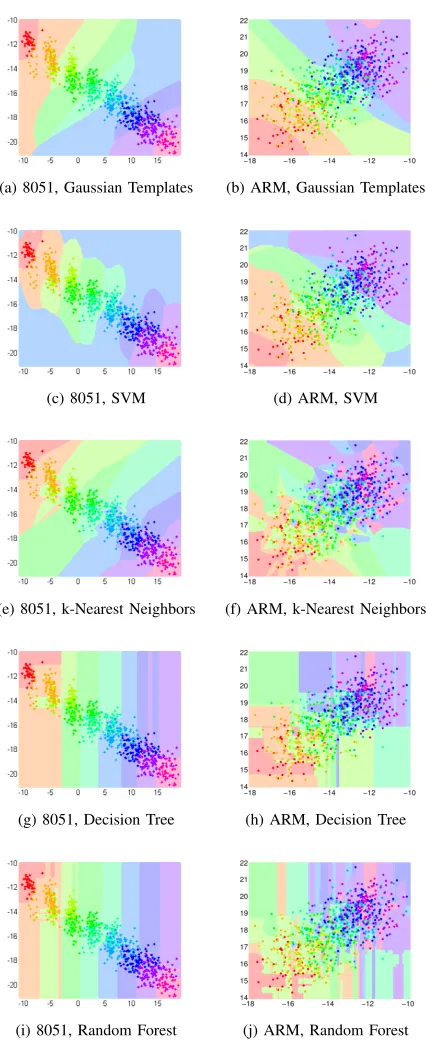
In order to get some intuition of the above methods, let us consider that the training data set is chosen from the 2-dimensional sets which are represented in Figure 1, say we choose both the 8051 and ARM data with POI. Let the testing data be, in each case, the grid of points that covers both axes spanned by the training data. Then, the decision surface of each classifier (see Figure 3) can be obtained by classifying each point on the corresponding grid as indicated by outputw1of that classifier. One can observe the interesting
behaviour of some classifiers, e.g. the DT basically implements some ranking of features, and a cut-off takes place at some point (this can be visualised through the rectangular-shaped surfaces). The RF classifier, which uses decision trees, has a similar but more granular decision surface. The kNN is highly sensitive to the local structure of the data.
IV. RESULTS
For the experiments we have varied the number of training traces from 25 to 500 per Hamming weight in steps of 25, and the number of POI as well as PC from 1 to 8, in steps of 1 (to be able to report consistent results for both devices and dimensionality reduction methods). For each scenario (20×8×2scenarios in total), we have generated50different training data sets, i.e. performed 50 independent experiments, and averaged out the results. We have used a fixed set of450
test traces for classification. The performance was evaluated by counting how many of the test traces were correctly ranked in the top s(see Section II).
The main issue that we address is whether it is at all possible to guarantee with certainty that the true leakage will be ranked within the top s by some classifier for the two concrete devices that we used. We can provide a positive answer to this question as several classifiers were able to achieve the required classification performance.
We now discuss the outcomes and focus on a number of practically relevant questions. We report some results of the experiments that were carried out using the RF classifier (the most efficient classifier that we have found), using POI, and setting s = 5 (which corresponds to the more challenging scenario in the exploitation phase, see Section II). The RF classifier was able to always identify the correct leakage in the top 5 for the simple microcontroller leakage, and by adjusting the parameters the classifier was also able to achieve the same classification performance in case of the complex microprocessor leakage.
A. Feasibility w.r.t. ASCA
(a) 8051, Gaussian Templates (b) ARM, Gaussian Templates
(c) 8051, SVM (d) ARM, SVM
(e) 8051, k-Nearest Neighbors (f) ARM, k-Nearest Neighbors
(g) 8051, Decision Tree (h) ARM, Decision Tree
(i) 8051, Random Forest (j) ARM, Random Forest
Fig. 3: Exemplary decision surfaces from training the classi-fiers. In the absence of a clear separation of classes, some algo-rithms struggle to find the optimum classification. NT = 250,
NP OI = 2.
we could not train any classifier to achieve this performance in the case of the ARM data sets.
B. Feasibility w.r.t. pragmatic SPA
For the microcontroller (8051), already a Gaussian template or SVM (even with a single POI or PC) will achieve the
TABLE I: ARM, RF: The confusion matrix. NT = 50,
NP OI = 2,s= 5.
Predicted class
0 1 2 3 4 5 6 7 8
Actual
class
0 1 0 0 0 0 0 0 0 0 1 0 1 0 0 0 0 0 0 0 2 0.03 0.03 0.68 0.06 0.06 0.04 0.03 0.03 0.02 3 0 0.01 0.02 0.78 0.04 0.04 0.04 0.04 0.01 4 0.03 0.02 0.04 0.05 0.68 0.06 0.04 0.04 0.02 5 0.02 0.03 0.02 0.04 0.05 0.70 0.03 0.04 0.02 6 0.01 0 0.01 0.04 0.04 0.04 0.78 0.03 0.03 7 0.01 0.01 0.01 0.01 0.01 0.02 0.02 0.89 0.01 8 0 0 0 0 0 0 0 0 1
desired performance. RF similarly can achieve the top 5 classification goal, however here providing either two POI or PCs is necessary. All our experiments showed that 25 training traces were sufficient to achieve an almost optimal classification performance, i.e. using more than 25 traces did not improve any of the classifiers.
Unsurprisingly, the results for the microprocessor (ARM) are quite different. Whilst Gaussian templates and SVM al-most achieve the desired performance, more training traces were required and more POI and PCs were necessary. RF is successful in some cases. Interestingly, there is a slight performance difference using the PC vs. the POI for the ARM data set. As discussed in Section III-A, the first principal com-ponent bears a higher correlation to the data than the highest correlation point, which leads to a performance difference for all classifiers.
Neither kNN nor DT could reach the desired classification performance for the data from our two target devices. This is in accordance with the intuition given in Section III-C.
Figure 4 shows the cumulative distribution functions for the probability that the true leakage is within the top s in the RF classifier output. The interesting values of s are 3
(corresponding to the set size required by error tolerant ASCA) and 5 (corresponding to the set size required by pragmatic SPA). Clearly for the simple microcontroller data we can succeed for both set sizes. However, in case of the more complex microprocessor data, only set size 5 can be achieved. We briefly focus on the scenarios in which the classifier fails to rank the correct leakage within the tops. Intuitively, middle classes (i.e., centred around HW = 4) overlap more, which could lead to a higher failure rate. This intuition is confirmed by the confusion matrix, in which element(i, j)evaluates the percentage of instances of classithat are classified as classj. Table I shows the confusion matrix for the RF classifier using ARM data, 50 training traces and two POI, fors= 5.
C. Impact of Noise
(a) 8051, increasingNT (b) 8051, increasingNP OI
(c) ARM, increasingNT (d) ARM, increasingNP OI
Fig. 4: RF: Cumulative distribution function of the probability that the true Hamming weight is contained within the top s, with sranging from 1 to9.NP OI = 6 (left) andNT = 250 (right).
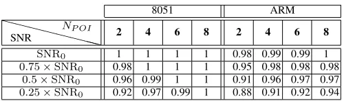
TABLE II: RF: The impact of noise on the classification performance;SNR0 is the original SNR.NT = 250,s= 5.
8051 ARM
XX XX
XXX X SNR
NP OI 2 4 6 8 2 4 6 8
SNR0 1 1 1 1 0.98 0.99 0.99 1
0.75×SNR0 0.98 1 1 1 0.95 0.98 0.98 0.98
0.5×SNR0 0.96 0.99 1 1 0.91 0.96 0.97 0.97
0.25×SNR0 0.92 0.97 0.99 1 0.88 0.91 0.92 0.94
Similarly for the microprocessor, we observed that lowering the signal had an impact on the classification performance, but the overall observations made before still apply: Gaussian templates, SVM and RF can be trained to achieve the desired performance. In the most noisy case that we considered (we lowered the natural SNR of the ARM data set by a factor of 4) we observed that the Random Forest method using POI achieved the best classification performance and almost reached the desired correct key rank; this implies too that none of the methods was (in the most noisy case) able to rank the true leakage under the topswith certainty. Table II shows the results using a training data set consisting of 250 traces.
V. CONCLUSION
We trained a number of classifiers with the aim of using them for the information (i.e. Hamming weight) extraction required as a precursor to pragmatic SPA and ASCA attacks. Such attacks are error tolerant to some extent: pragmatic SPA can tolerate a set size of up to 5 and ASCA can tolerate a set size of up to 3. We used data from two devices (a microcon-troller based on an 8051 instruction set and a microprocessor based on an ARM7 core) that would be a typical target for such attacks. The data from the 8051 were raw traces, which feature a very clear Hamming weight leakage with little noise. The data from the ARM were filtered to improve the SNR. It leaks proportional to the Hamming weight but both contains
more noise than the 8051 (despite filtering) and exhibits less clearly defined Hamming weight features.
Due to the fact that the microcontroller data is ‘nice’, it was possible to train some classifiers to meet both the requirements of pragmatic SPA and ASCA. The picture for the ARM data was different: only Gaussian templates, SVM, and RF were capable of achieving the classification performance required for pragmatic SPA attacks. It was not possible to achieve the performance required for ASCA with any classifier in case of the ARM data. This leads us to conclude that the practical relevance of such SPA style attacks is still limited, albeit the more error tolerant nature of pragmatic SPA gives it a natural advantage over ASCA.
REFERENCES
[1] S. Mangard, “A simple power-analysis (SPA) attack on implementations of the AES key expansion,” in Information Security and Cryptology (ICISC) 2002. Springer, 2003, pp. 343–358.
[2] M. Renauld and F.-X. Standaert, “Algebraic side-channel attacks,” in
Information Security and Cryptology (INSCRYPT) 2009. Springer, 2009, pp. 393–410.
[3] M. Renauld, F.-X. Standaert, and N. Veyrat-Charvillon, “Algebraic side-channel attacks on the AES: Why time also matters in DPA,” in Cryp-tographic Hardware and Embedded Systems-CHES 2009. Springer, 2009, pp. 97–111.
[4] V. Banciu and E. Oswald, “Pragmatism vs. elegance: comparing two approaches to simple power attacks on AES.”IACR Cryptology ePrint Archive, vol. 2014, p. 177, 2014.
[5] Y. Oren, M. Kirschbaum, T. Popp, and A. Wool, “Algebraic side-channel analysis in the presence of errors,” in Cryptographic Hardware and Embedded Systems-CHES 2010. Springer, 2010, pp. 428–442. [6] S. Chari, J. R. Rao, and P. Rohatgi, “Template attacks,” inCryptographic
Hardware and Embedded Systems-CHES 2002. Springer, 2003, pp. 13– 28.
[7] C. Rechberger and E. Oswald, “Practical template attacks,” in Informa-tion Security ApplicaInforma-tions. Springer, 2005, pp. 440–456.
[8] G. Hospodar, B. Gierlichs, E. De Mulder, I. Verbauwhede, and J. Vande-walle, “Machine learning in side-channel analysis: A first study,”Journal of Cryptographic Engineering, vol. 1, no. 4, pp. 293–302, 2011. [9] L. Lerman, G. Bontempi, and O. Markowitch, “Side channel attack:
An approach based on machine learning,” inConstructive Side-Channel Analysis and Secure Design. Springer, 2011, pp. 29–41.
[10] A. Heuser and M. Zohner, “Intelligent machine homicide,” in Construc-tive Side-Channel Analysis and Secure Design. Springer, 2012, pp. 249–264.
[11] C. Archambeau, E. Peeters, F.-X. Standaert, and J.-J. Quisquater, “Tem-plate attacks in principal subspaces,” inCryptographic Hardware and Embedded Systems-CHES 2006. Springer, 2006, pp. 1–14.
[12] C. Cortes and V. Vapnik, “Support-vector networks,”Machine Learning, vol. 20, no. 3, pp. 273–297, 1995.
[13] B. Sch¨olkopf and A. J. Smola,Learning with kernels: support vector machines, regularization, optimization, and beyond. MIT press, 2002. [14] L. Breiman, “Random forests,”Machine Learning, vol. 45, no. 1, pp.
5–32, 2001.