Endogeneity in semiparametric binary response models

Endogeneity in Semiparametric Binary

Response Models

Richard Blundell

and James L. Powell

July 2001

Revised, September 2003

Abstract

This paper develops and implements semiparametric methods for es-timating binary response (binary choice) models with continuous endoge-nous regressors. It extends existing results on semiparametric estimation in single index binary response models to the case of endogenous

regres-sors. It develops a control function approach to account for endogeneity

in triangular and fully simulataneous binary response models. The pro-posed estimation method is applied to estimate the income effect in a labor market participation problem using a large micro data set from the British FES. The semiparametric estimator is found to perform well, detecting a significant attenuation bias. The proposed estimator is contrasted to the corresponding Probit and Linear Probability specifications.

JEL: C14, C25, C35, J22.

Key Words: Binary Response, Probit, Endogeneity, Semiparametric Estimation.

Address for correspondence: Richard Blundell, Department of Economics, University College London, Gower Street, London, WC1E 6BT, UK. email: [email protected]

∗_{University College London, Department of Economics, Gower Street, London, WC1E 6BT}

and Institute for Fiscal Studies. [email protected]

1. Introduction

This aim of this paper is to develop and implement semiparametric methods for estimating binary response models with endogenous regressors. The case of in-terest here is a single index model for a binary dependent variable with continuous endogenous regressors. Other covariates and the instrumental variables may be discrete. This paper extends the extensive literature dealing with semiparametric estimation in single index binary response models to the continuous endogenous regressor case. It highlights the attractiveness of the control function approach, which introduces residuals from the reduced form for the regressors as covariates in the binary response model to account for endogeneity in this framework.

on the control function approach to nonparametric estimation with endogenous regressors. In nonlinear models this differs from the standard assumption of the instrumental variable (IV) approach — namely, that the instrumental variables are independent of the error term in the equation of interest. In the binary response model the parameters of interest in semi- and nonparametric binary response mod-els are not identified in general under the standard IV assumption (see Blundell and Powell 2003); however, we show that many of these parameters, including the index coefficients and average structural function (ASF), are identified through the control function assumptions we consider here. While our general approach is amenable to implementation using any of a number of estimation methods for single index models, this paper focuses on a particular single-index estimator pro-posed by Ahn, Ichimura, and Powell (1996), which is modified to accommodate endogenous regressors.

is large. Third, a participation rate of 85% suggests that parametric model results may be sensitive to distributional assumptions which differ in their specification of tail probabilities. We find a strong effect of correcting for endogeneity in this example and show that adjusting for endogeneity using the standard parametric models, the Probit and linear probability models, give a highly misleading picture of the impact on participation of an exogenous change in other income.

As an alternative representation of the simultaneous binary response model, we also consider a framework which corresponds to a “fixed costs of work” repre-sentation of the participation decision. This is a fully simultaneous specification in which the binary outcome enters directly in to the model for other income. It corresponds to an economic model in which decision making is over observed outcomes. In this case there is no explicit reduced form for other income since the fixed cost of work is subtracted from income when working. Consequently this specification does not permit a triangular representation and turns out to be a special case of the coherency model framework for dummy endogenous mod-els developed for the simultaneous Probit model by Heckman (1978). Blundell and Smith (1994) considered the control function approach for estimation in the joint normal model. We show that our semiparametric framework is equally well suited to this fully simultaneous specification of the binary response model with endogenous regressors.

correction of endogeneity of other income in the participation decision. The cor-rection for endogeneity is found to be important and the estimated effect is shown to be strongly biased when inappropriate parametric distributional assumptions are imposed. Section 5 develops the implementation of our approach to the fully simultaneous coherency model which allows for fixed costs of participation. Sec-tion 6 concludes.

2. Model Speci

fi

cation

In this paper we consider the binary response model

y1i = 1{y1∗i >0}, (2.1)

where the latent variable y∗

1 is assumed to be generated from a linear model of

the form

y1∗i =xiβ0+ui, (2.2)

wherexi is a (row) vector of explanatory variables for observationsi= 1, ..., n,ui

is an unobservable scalar error term, and the conformable column vectorβ₀ of un-known regression (“index”) coefficients is defined up to some scalar normalization (possibly involving the distribution of ui). If ui were assumed to be independent

of xi, with (possibly unknown) distribution function Pr{−ui ≤ λ} = G(λ), the

binary variable y1i would satisfy a “single index regression” model of the form

E[y1i |xi] =G(xiβ0), (2.3)

In some settings, though, the assumption of independence of the error term

ui and the regressors xi would be suspect, if some components of xi (denoted

y2i here) were determined jointly with the latent variable y1∗i, as in the usual

simultaneous equations framework. That is, endogeneity in some components of x might be accommodated through the following recursive structural form:

y1i = 1{xiβ0+ui >0}

= 1_{z1iβ1+y2iβ2+ui >0}, (2.4)

wherexi ≡(z1i,y2i) is of dimension(1×(p+q)), theq-vectory2i is assumed to

be determined by the reduced form

y2i = E[y2i|zi] +vi (2.5)

≡ π(zi) +vi,

and the vector of instruments

zi ≡(z1i,z2i) (2.6)

is of dimension 1_×(p+m), with m _≥ q. (Here m ₋q describes the degree of overidentification.) By construction, the reduced form error terms vi have

E(vi|z_i) =0, (2.7)

though alternative centering assumptions (e.g., conditional median zero) would be compatible with the approach taken here.

If the joint distribution of the structural error termui and reduced form error

termsvi were parametrically specified (as, say, Gaussian and independent of zi),

maximum likelihood estimation could be applied to obtain consistent estimators ofβ₀,π(_·), and the unknown parameters of the joint distribution function of the errors. To be specific, assuming a joint normal distribution for the error terms and a particular normalization for V ar(u),we have

E(y1i|xi,vi) = Pr[ui >−xiβ|v_i]

= Φ(xiβ+ρvi), (2.8)

where ρ is the vector of population regression coefficients of ui on vi. The

para-meters β and ρ can be estimated directly from the conditional likelihood for y1i

givenxi andvi. Blundell and Smith (1986) show that, unlike in the linear model

case, this “control function” approach is asymptotically more efficient in discrete and censored normal models than an alternative two-stage estimation approach.

In a semiparametric setting, where the joint error distribution and reduced form regression functions are not parametrically specified, one possible “two stage” estimation approach would insert the reduced form for y2i into the structural

model (2.4), yielding

y1i = 1{z1iβ1+π(zi)β2+ui+viβ0 >0}, (2.9)

which would yield a single index representation

E[y1i|zi] =H(π(zi)β0), (2.10)

assuming the composite error term ui + viβ0 is independent of zi with c.d.f.

H(₋λ).While a two-stage estimation approach (using a nonparametric estimator of π(zi) in the first stage) could be used to consistently estimate the parameters

term ui +viβ0 might be difficult to maintain, particularly if the reduced form

error terms vi do not appear to be independent of the instruments (as might

be revealed by standard tests for heteroskedasticity, etc.). Moreover, this ‘fitted value’ approach does not easily yield an estimator of the marginal c.d.f. G(_·) of the error terms ₋ui, which would be needed to evaluate the effect on response

probabilities of an exogenous shift in the regressorsxi.

An alternative approach to estimation of the components of this model, adopted here, uses estimates of the reduced form error terms vi as “control variables” for

the endogeneity of the regressors in the original structural equation. The key identifying assumptions for estimation of the unknown coefficientsβ and the dis-tribution function of the error term ui is a distributional exclusion restriction,

which requires that the dependence of the structural error term ui on the vector

of regressors xi and instrumental variables zi is completely characterized by the

reduced form error vectorvi : that is,

ui|xi,zi ∼ ui|xi,vi (2.11)

∼ ui|vi, (2.12)

where the tilde symbol denotes equality of conditional distributions. Under this last condition, the conditional expectation of the binary variable y1i given the

regressorsxi and reduced form errors vi takes the form

E[y1i|xi,vi] = Pr[−ui ≤xiβ0|xi,vi]

= F(xiβ0,vi), (2.13)

whereF(_·,vi)is the conditional c.d.f. of−ui givenvi.Thus,y1i can be

xi and vi, that depends upon xi only through the single index xiβ0. As in the

single index regression model, it is the dimensionality reduction in the conditional expectation ofy1i givenxi andvi that can be exploited to obtain a√n-consistent

estimator of the index coefficientsβ₀.

Our approach to identification and estimation of the unknown regression

coef-ficientsβ0 uses an extension of the Ahn, Ichimura and Powell (1996) “matching”

estimator of β0 for the single index model without endogeneity. This approach,

adapted to the present context, assumes both the monotonicity and continuity of

F(xiβ,vi)in itsfirst argument. Since the structural index model is related to the

conditional mean ofy1i given wi= (x_i,vi) by the relation

E[y1i|xi,vi]≡g(wi) =F(x_iβ0,vi), (2.14)

invertibility of F(_·) in its first argument implies

xiβ0−ψ(g(wi),vi) = 0, (w.p.1), (2.15)

where ψ(_·,v)_≡F−1(_·,v) , i.e.,

F(ψ(g,v),v) =g. (2.16)

If two observations (with subscriptsiandj) have identical conditional means (i.e.,

g(wi) = g(wj)) and identical reduced form error terms (vi =vj), it follows that

their indicesxiβ0 andxjβ0 are also identical:

(xi−xj)β0 = ψ(g(wi),vi)−ψ(g(wj),vj)

= 0 if (2.17)

So, for any nonnegative functionω(wi,wj)of the conditioning variables wi and

wj, it follows that

0 = E[ω(wi,wj)·((xi−xj)β0)2 |g(wi) =g(wj),vi =vj]

≡ β0₀Σwβ0, (2.19)

where

Σw ≡E[ω(wi,wj)·(xi−xj)0(xi−xj)|g(wi) =g(wj),vi =vj]. (2.20)

That is, the nonnegative-definite matrix Σwis singular, and the unknown

parame-ter vectorβ0 is the eigenvector (with an appropriate normalization) corresponding

to the zero eigenvalue of Σw. Under the identifying assumption that Σw has

rank p+q₋1 = dim(x)₋1 — which requires that any nontrivial linear combi-nation (xi−xj)λ of the difference in regressors has nonzero conditional variance

whenλ6=β0 — the parameter vector β0 as the eigenvector corresponding to the

unique zero eigenvalue ofΣw . We construct an estimator ofβ0 as the eigenvector

corresponding to the smallest eigenvalue (in magnitude) of a sample analogue to theΣw matrix, for a convenient choice of the weighting function ω(·).

In addition to the vector of regression coefficientsβ0 (defined up to some scale

normalization), the other key parameter of interest is the marginal probability distribution function of the structural errors₋ui,

G(λ) = Pr[₋ui ≤λ]; (2.21)

when λ = xβ0, we define this function G(xβ0) to be the Average Structural

is the marginal response to an exogenous shift in x. The marginal distribution function G(λ) of ₋ui can be identified as the “partial mean” of this conditional

distribution function F(xβ₀,vi), holding the indexxβ0 fixed and averaging over

the marginal distribution of the reduced form errorsvi:

G(xβ₀) =

Z

F(xβ₀,v)dFv. (2.22)

And, given a particular marginal distribution F∗

x for the regressors x of

inter-est (including possibly the observed marginal distribution), the average response probability for exogenous regressors with that distribution would be

γ∗ _≡

Z

G(xβ0)dFx∗, (2.23)

which may be of interest for policy analysis (Stock 1989).

3. Estimation

3.1. The semiparametric estimation approach

The approach adopted here for estimation of the parameters of interest in this model follows three main steps. Thefirst step uses nonparametric regression methods to estimate the error term vi in the reduced form, as well as the

unrestricted conditional mean of y1i given xi and vi,

E[y1i|z1i,y2i,vi] ≡ E[y1i|xi,vi] (3.1)

≡ E[y1i|wi]

≡ g(wi)

wherewi is the 1×(p+ 2q)vector

This step can be viewed as an intermediate ‘structural estimation’ step, which imposes thefirst exclusion restriction of (2.11) and (2.12) but not the second.

The second step imposes the linear index assumptions on the unrestricted conditional mean

E[y1i|z1i,y2i,vi] ≡ E[y1i|xi,vi] (3.3)

= E[y1i|xiβ0,vi]

≡ F(xiβ0,vi)

to obtain an estimator βˆ of β₀.

The final step recovers an estimator of G(xβ0) ≡ R

F(xβ0,v)dFv. It is

ob-tained by computing a sample average of Fˆ(λ,vi) over the observations, holding

λfixed and substituting the estimates ˆvi for vi, an application of “partial mean”

estimation (Newey 1994).

3.2. Implementation of the estimation approach

Let_{(yi,zi)}ni=1be a random sample of observations from the model described

above. In estimation of the conditional mean ofy1i, vi is replaced by the residual

from the nonparametric regression of y2i on zi, so that in place of (3.2) we have

b

wi = (xi,y2i−πb(zi)) (3.4)

≡ (xi,vˆi),

where πb(zi) is the unrestricted Nadaraya-Watson kernel regression estimator for

the mean of xi given zi.

regression estimator

b

g(w_bi)≡fb(wbi)−1r(bwbi), (3.5)

with

b

r(w_bi) ≡

1 n

X

j

Kw(wbi−wbj)y1j, (3.6)

b

f(wbi) ≡

1 n

X

j

Kw(wbi−wbj), (3.7)

whereKw(ζ) =h−

(p+2q)

w K(ζ/hw)for bandwidthhnsatisfyinghw →0andnhpw+2q →

∞as n_{→ ∞}, and some kernel function K :Rp+2q

→R+ _{that satisfies standard}

conditions like RK(ζ)dζ = 1.

Given the preliminary nonparametric estimators vbi and bg(wbi) of vi and

g(wi) defined above, and assuming smoothness (continuity and differentiability)

of the inverse function ψ(_·) in (2.16), a consistent estimator of Σw for a particular

weighting function ω(wi,wj) can be obtained by a ‘pairwise differencing’ or

‘matching’ approach which takes a weighted average of outer products of the differences (xi −xj) in the

¡n

2 ¢

distinct pairs of regressors, with weights that tend to zero as the magnitudes of the differences _|bg(w_bi)−bg(wbj)| and |vi−vj|

increase. As in Ahn, Ichimura, and Powell (1996), the estimator of Σw is defined

as

ˆ Sw ≡

µ

n 2

¶−1_X

i<j

b

ωij(xi−xj)0(xi−xj), (3.8)

for

ˆ

ωij ≡h−nq+1Kg

µ b

g(w_bi)−bg(wbj)

hn

¶

Kv

µ ˆ vi−ˆvj

hn

¶

titj, (3.9)

where Kg and Kv are kernel functions analogous to the kernel function Kw

the conditioning variables zi and wbi lie outside a compact set. As the sample

size n increases, and the bandwidth hn shrinks to zero, the weighting term ωbij

tends to zero, except for pairs of observations with_bg(w_bi)'bg(wbj) and ˆvi 'ˆvj.

With this estimator of the matrix Σw, a corresponding estimator βb of β0

can be defined as the eigenvector corresponding to the eigenvalue ˆη of Sˆw that

is closest to zero in magnitude. (Because the kernel functions Kg and Kv will

be permitted to become negative for some values of their arguments, we choose the eigenvalue closest to zero, rather than the minimum of the eigenvalues.) A convenient normalization of this eigenvector sets the first component to unity; that is, we normalize

β₀ =

µ

1

−θ0

¶ , βˆ = µ 1 −ˆθ ¶ , (3.10)

and, partitioning Sˆ conformably as

ˆ Sw=

· _ˆ

S11 ˆS12

ˆ

S21 ˆS22 ¸

, (3.11)

the estimator of the subvector θ0 can be written as

ˆ

θ = [Sˆ22−ˆηI]−1Sˆ21, (3.12)

where

ˆ

η _≡arg min

α:kαk=1|

α0Sˆwα|. (3.13)

Using the estimator βb, we can estimate the index as bλ = xβb for any value of x, which we can then use to estimate the average structural function G(xβ0),

the marginal probability thaty1i = 1given an exogenousx. The joint probability

functionF(xβ0,v)can be directly estimated through a nonparametric (kernel)

function G(xβ0) from a sample average ofFb(xβb,bvi)over ˆvi,

b

G(xβb) =

n

X

i=1 b

F(xβb,v_bi)τi, (3.14)

where τi =τ(bvi, n) is some ‘trimming’ term which downweights observations for

which Fb(_·) is imprecisely estimated.

3.3. Alternative assumptions and estimators

Given the assumptions imposed in section 2 above, several variations on the es-timation strategy outlined in the previous section might be adopted. For example, to obtain thefirst-stage estimates of the conditional mean functiong(wi) =E[y1i|wi]

and residuals vi = xi−E[xi|zi], more sophisticated nonparametric regression

methods like local polynomial regression might be used instead of the simpler kernel estimators adopted here. And, given a √n-consistent estimator βb of β,

an alternative to the “partial mean” estimator of the average structural function

b

G(λ) could be based upon “marginal integration” of Fˆ(λ,v), weighting by the estimated joint density functionfbv(v) forvi,

e

G(λ) =

Z b

F(λ,v)fbv(v)dv, (3.15)

as discussed by Linton and Nielson (1995) and Tjosthiem and Auestad (1994).

For estimation ofβ0,the index coefficients, the multi-index restrictionE[y1i|xi,vi] =

F(xiβ0,vi) can be exploited with modification of most existing single-index

esti-mation methods. The “average derivative” (Härdle and Stoker 1989) or “weighted average derivative” (Powell, Stock, and Stoker 1989) estimation methods for single index models could be adapted to estimation ofβ₀ here, using the fact that

E

·

w(xi,vi)·

∂E[y1i|xi,vi]

∂x ¸

=β0·E

·

w(xi,vi)·

∂F(xiβ,vi)

∂(xβ)

¸

With these estimators, as with the recent proposal by Hristache, Juditsky, and Spokoiny 2001 (which combines average derivative and local linear regression es-timation), the function F(_·) need not be assumed to be monotonic in xiβ0, but

all components of xi must be continuously distributed, which is uncommon in

empirical applications, including the one presented herein. Other possibilities in-clude generalizations of the single-index regression estimator of Ichimura (1993) or semiparametric binary response estimator of Klein and Spady (1993); these would fit the nonlinear regression function E[y1i|xi,vi] = F(xiβ0,vi) iteratively

by either nonlinear least squares or binary response maximum likelihood, using nonparametric regression to estimate F(xib,vi) as a function of b. Like the

av-erage derivative estimators, these estimators would not need the monotonicity re-quirement, can accommodate discontinuous regressors,involves lower-dimensional nonparametric regression, and can be more statistically efficient. However, while each nonparametric regression step involves a lower-dimensional regression (to es-timate E[y1i|xib,vi] rather than E[y1i|xi,vi]), iteration between estimation of F

and minimization or maximization over b makes these estimators less computa-tionally tractable than the present estimator. Yet another candidate would be a “local probit” estimator which estimated the reparametrised function

F(xβ₀,v)_≡Φ(xβ(x,v) +vρ(x,v)) (3.17)

in a neighborhood of each value of xi and vbi (where Φ is the standard normal

cumulative) by maximizing a local likelihood

L(β,ρ;w)_≡

n

X

i=1

Kw(w−wbi) [y1iln(Φ(xβ+vρ)) + (1−y1i) ln(1−Φ(xβ+vρ))];

given local estimators βb(wb) = bβ(x,vb) of the slope coefficients, the index coeffi -cients β₀ could be recovered by integration,

e β =

Z b

β(x,v)dFb(x,v), (3.19)

and the parametric might model could be tested as a special case by testing the constancy of the estimated ρ(x,v)function.2

All of these alternative index coefficient estimators, like the ones proposed here, are based upon the multi-index regression function E[y1i|xi,vi] = F(xiβ0,vi),

which in turn are derived from the distributional exclusion restrictions (2.11) and (2.12), which are the basis for the control function approach; thus, they all share in some restrictive aspects of those assumptions. First, as for single-index estimators of binary response models without endogeneity, the form of permissible heteroskedasticity in the structural error ui is limited to functions of xiβ0 andvi,

ruling out, e.g., regressors with random coefficients. Also, location of the error termui is not identified, though this is only because no location restriction onui

is imposed by the exclusion restrictions, and location parameters forui could be

recovered directly from the ASF G(λ).

More fundamentally, in contrast to the linear model, consistency of the control function approach for the binary response and other nonlinear models requires a correct, or at least complete, specification of the vector zi of instruments for

the first-stage nonparametric regression. In the linear model with endogenous regressors, least-squares regression of the dependent variable on the endogenous variables and first-stage residuals yields the two-stage least squares estimators as the estimated regression coefficients, so any set of valid instruments satisfying

the relevant rank condition will yield consistent estimators; in general, though, the conditional independence restrictions (2.11) and (2.12) will no longer hold in general ifzi is replaced by a subvector, so “correct” specification of thefirst stage

is essential. Also, as discussed in more detail by Blundell and Powell (2003), es-timation of the multi-index regression function F(xiβ0,vi) and its partial mean,

the ASFG(xiβ0), requires thefirst-stage residualvi (and thus the endogenous

re-gressors) to be continuously distributed, which holds for our empirical application but not more generally.

If the primary interest is in the index coefficients β0, rather than the ASF G(xβ₀), it may be identified and consistently estimated under weaker conditions than the conditional independence restrictions (2.11) and (2.12). Consider, for example, replacing the distributional exclusion restrictions with the corresponding median exclusion restrictions

med_{ui|xi,zi} = med{ui|xi,vi}

= med_{ui|vi} (3.20)

≡ η(vi),

which restrict only the 50th percentiles of the corresponding conditional distribu-tions. Under these restrictions,

med_{y1i|xi,vi}= 1{xiβ0+η(vi)}, (3.21)

and estimation of β0 might be based upon a generalization of Manski’s (1975,

of the ASF, though, would require strengthening of the median exclusion restric-tions to independence restricrestric-tions.

When the regressor vectorxi includes a (scalar) exogenous variablez0i which is

continuously distributed with a large support, it is possible to derive√n-consistent estimators of β under substantially weaker versions of the exclusion restrictions (2.11) and (2.12), using the approach proposed by Lewbel (2000) and its variants (Lewbel 1998, Honoré and Lewbel 2001). Writing the vector of regressors as xi≡(z0i,z1i,y2i), the distributional exclusion restrictions can be relaxed to the

form

ui|xi,zi ∼ ui|z1i,y2i,vi (3.22)

∼ u_|z1i,π(zi),y2i (3.23)

which is supplemented by the unconditional moment restrictions

E[z1iui] = 0, (3.24)

E[π(z_i)ui] = 0, (3.25)

whereπ(z_i)_≡E[y2i|zi].Under this combination of conditional independence and

unconditional moment restrictions, Lewbel (2000) shows that a linear least-squares regression of[y1i−1{z0i >0}]/f(z0i|z1i,π(z_i),y_2i) onz1i andπ(z_i),where f(·) is

the conditional density of the “special regressor”z0i (which must be replaced by a

consistent estimator in practice), yields a consistent estimator of the “normalized” coefficients θ0 from (3.10). Additional restrictions on z0i (e.g., its independence

from π(z_i), or from ui and the other regressors) permit more general forms of

continuously-distributed, exogenous regressor in the binary response equation (which is not available in our empirical example), it would accommodate discrete endogenous regressors, unlike the control function approach. Hence, the two approaches to es-timation ofβ₀ may be viewed as complementary, depending upon whether the en-dogenous or exogenous regressors are continuously distributed,4 _{and either might}

be combined with the “partial mean” approach to estimation of the ASFG(xβ0),

which represents the response probability for an exogenously-specified regression vector x. Our choice of the Ahn, Ichimura, and Powell (1996) generalization is motivated by its applicability to our empirical problem and its computational simplicity compared to competing procedures.

3.4. Large-sample properties of the proposed estimators

The objectives of the asymptotic theory for the estimators proposed here are,

first, demonstration of consistency and asymptotic normality of the estimator ˆ

β of β₀ and, second, demonstration of (pointwise) consistency of the marginal distribution function estimator G(λ).b Derivation of the asymptotic distribution of

ˆ

β will be similar to that for the ‘monotone single index’ estimator proposed by Ahn, Ichimura and Powell (1996); the present derivation is more complex, both in analysis of the first stage estimator of g(wi) (since the estimated residuals ˆvi

are used as covariates in a nonparametric regression step) and in the second stage estimatorSˆw of Σw, which must condition on the reduced-form residuals as well

as the preliminary estimatorsgˆi ∼= ˆg(w˜i) andvˆi ≡y2i−πˆ(zi)≡y2i−πˆi.

of the matrix ˜Sw for Σw, plus an identification condition. Making a first-order

Taylor’s series expansion around the true valuesgi ≡g(wi)andvi,the matrixSˆw

can be decomposed as

ˆ

Sw =S0+S1, (3.26)

where

Sl ≡

µ

n 2

¶−1_X

i<j

ωlij(xi−xj)0(xi−xj), l = 0,1, (3.27)

ω0ij ≡h−n(q+1)Kg

µ_g

i−gj hn

¶

Kv

µ

vi−vj

hn

¶

titj, (3.28)

and

ω1_{ij ≡} h−_n(q+2)K_g(1)

µ_g∗

ij

hn

¶

Kv

µ_v∗

ij

hn

¶

(ˆgi−g˙i−gˆj +gj)titj

−h−_n(q+2)Kg

µ_g∗

ij

hn

¶

K_v(1)

µ_v∗

ij

hn

¶

(πˆi−πi−πˆj −πj)0titj. (3.29)

In these expressions, the superscript ‘(1)’ denotes the (row) vectors offirst deriva-tives of the respective kernel functions, whileg∗

ij andvij∗ denote intermediate value

terms.

The leading-order term S0 is the simplest to analyze, since it is in the form

of a second-order U-statistic (with kernel depending upon the sample size n). It is straightforward to show that the first two moments of the summand in S0 are

of order hq+1

n (for q the dimension of y2i, the vector of endogenous regressors),

provided the regressors xi have four moments and the trimming terms ti and

kernel functions Kg(·) and Kv(·) are bounded. Thus, by Lemma 3.1 of Powell,

Stock and Stoker (1989), if

then

S0−E[S0] =op(1). (3.31)

Furthermore, with continuity of the underlying conditional expectation and den-sity functions, it can be shown that, asn_{→ ∞} (and hn→0),

E[S0]→Σw ≡E[2f(gi,vi)·(τiνi−µ0iµi)|gi =gj,vi =vj], (3.32)

wheref(g,v) is the joint density function of gi ≡g(wi) andvi,, and where

τi ≡ E[ti|gi,vi],

µi ≡ E[tixi|gi,vi], and

νi ≡ E[tix0ixi|gi,vi]. (3.33)

If the preliminary estimators ˆgi and πˆi converge at a sufficiently fast rate, and if

the levels and derivatives of the kernel functions Kg(·) and Kv(·) are uniformly

bounded, the termS1 will be asymptotically negligible. More precisely, assuming

max

i ti[|gˆi−gi|+||πˆi−πi||] =op(h q+2

n ) (3.34)

and the levels and derivatives of the kernels are bounded,

||K_g(l)_||+_||K_v(l)_||< C, j = 0,1, some C, (3.35)

then it is simple to show that

S1 =op(1). (3.36)

bias-reducing’ kernel functions, the dimensionality of the vectorsxi,vi,andzi,and

particular convergence rates for the bandwidths of the first-stage nonparametric estimators.

Thus, if these conditions hold, it follows that

ˆ

Sw =Σw +op(1). (3.37)

Moreover, by the identity (2.15), it follows that

(τiνi−µ0iµi)β0 = τiE[tix0ixiβ0 |gi,vi]−µ0iE[tixiβ0 |gi,vi]

= τiE[tix0i |gi,vi]ψ(gi,vi)−µ0iE[ti |gi,vi]ψ(gi,vi)

= 0, (3.38)

so that the limit matrixΣw is indeed singular with

Σwβ0 = 0, (3.39)

as required. The consistency argument is completed with an assumption thatβ0

is the unique nontrivial solution to the system of homogeneous linear equations (3.39), i.e.,

Σwλ= 0, λ6=β0 =⇒λ=0. (3.40)

This in turn implies a ‘full rank’ condition for the conditional expectations πi =

E[y2i|zi], since (3.40)

Pr_{(xi−xj)λ 6= 0|vi =vj,(xi−xj)β0 = 0,λ6=β0,λ6=0}

= Pr_{(πi−πj)λ6= 0|vi =vj,(πi−πj)β0 = 0,λ6=β0,λ6=0}

where the equality follows from the identityxi ≡πi+vi.

Since eigenvalues and (normalized) eigenvectors are continuous functions of their matrix arguments, the assumptions and calculations above yield weak con-sistency of the estimatorβˆ, i.e.

ˆ

β=β0 +op(1). (3.42)

Establishing the √n-consistency and asymptotic normality of βˆ would require a more refined asymptotic argument, based upon a second-order Taylor’s series expansion of the matrix Sˆw,

ˆ

Sw =S0+S1+S2, (3.43)

where, as before,

Sl ≡

µ

n 2

¶−1_X

i<j

ωl_ij(xi−xj)0(xi−xj), l = 0,1,2, (3.44)

with

ω0ij ≡h−

(q+1)

n Kg

µ_g

i−gj hn

¶

Kv

µ

vi−vj

hn

¶

titj, (3.45)

as before, but now

ω1_{ij ≡} h−_n(q+2)K_g(1)

µ

gi−gj

hn

¶

Kv

µ

vi−vj

hn

¶

(ˆgi−g˙i−gˆj +gj)titj

−h−_n(q+2)Kg

µ

gi−gj hn

¶

K_v(1)

µ

vi−vj

hn

¶

and

ω2_{ij ≡} h −(q+3)

n

2 K

(2)

g

µ_g∗

ij

hn

¶

Kv

µ_v∗

ij

hn

¶

(ˆgi−g˙i−gˆj+gj)2titj

−h−_n(q+3)(ˆgi−gi −gˆj+gj)Kg(1)

µ_g∗

ij

hn

¶

K_v(1)

µ_v∗

ij

hn

¶

·(πˆi−πi−πˆj+πj)0titj (3.47)

+h

−(q+3)

n

2 (πˆi−πi−πˆj+πj)Kg

µ_g∗

ij

hn

¶

K_v(2)

µ_v∗

ij

hn

¶

·(πˆi−πi−πˆj+πj)0titj. (3.48)

Since demonstration of√n-consistency ofβˆinvolves normalization of each of these terms by the factor √n, the regularity conditions would have to be strengthened substantially, with considerably more smoothness of the unknown density and ex-pectation functions, a higher rate of convergence of the preliminary nonparametric estimators, bias-reducing kernels of yet higher order, and a more restricted rate of convergence of the second-step bandwidth to zero. Still, with appropriate

modi-fication of the conditions and calculations in Ahn, Ichimura, and Powell (1996), the terms S0 and S2, when postmultiplied by the true parameter vector β0, and

appropriately normalized, should be asymptotically negligible,

√

nS0β0 =op(1) =

√

nS2β0, (3.49)

while thefirst-order component matrix S1 should satisfy an asymptotic linearity

relation of the form

√

nS1β0 = √

nSˆwβ0+op(1) (3.50)

= √1 n

n

X

i=1

with

e1i ≡2τif(gi,vi)·(τixi−µi)0·

∂ψ(g(wi),vi)

∂g ·(y1i−g(wi)) (3.52)

being the component of the influence function forSˆwβ0 due to the nonparametric

estimation of gi ≡E[y1i|xi,vi] and

e2i ≡ −E

·

2τif(gi,vi)·(τixi−µi)0·

∂ψ(g(wi),vi)

∂v0 |zi

¸

·vi (3.53)

being the influence function component accounting for the first-stage nonpara-metric estimation ofvi ≡y2i−E[y2i|zi].

Given the validity of (3.51), the same argument as given for (3.38) would yield

√

nβ0₀ˆSwβ0 =op(1), (3.54)

from which the √n-consistency and asymptotic normal distribution of the lower

(p+q₋1)-dimensional subvectorbθ of βb,

√

n(θb₋θ0)

d

→N(0,Σ−₂₂1V22Σ−221), (3.55)

will follow from the same argument as in Ahn, Ichimura, and Powell (1996), with

V_≡E[(e1i +ei2)(e1i+e2i)0] (3.56)

and withΣ22 andV22 the lower (p+q−1)×(p+q−1)diagonal submatrices of

Σw andV,as in (3.11).

Demonstration of consistency and asymptotic normality of the estimatorG(b xβb)

by Newey (1994). First, while Newey’s results assumed the trimming term τi in

(3.14) to be independent of the sample size (so that a positive fraction of ob-servations is trimmed in the limit, to help bound the denominator of the kernel regression away from zero), it would be important to extend the results to permit

τi = τi(vbi, n) to tend to unity as n → ∞ for all i. This would ensure that the

probability limit of G(b xβb) is an expectation, and not a truncated expectation, of

F(xβ,v_i) over the marginal distribution ofvi.5

Another important extension of Newey’s partial-mean results would account for the use of estimated regressors in the nonparametric estimation of the nonlinear regression functionF(xiβ0,vi).While these results would directly apply to kernel

regressions of y1i on the true index xiβ0 and control variable vi, they do not

account for the added imprecision due to the semiparametric estimator βb of the index coefficients, nor of the nonparametric estimator_bviof thefirst-stage residuals.

While the “delta method” approach taken by Newey could, in principle, be used to derive variance estimators in this case, it is difficult to obtain analytic formulae using this approach.

ymptotically normal). Moreover, based upon formal calculations analogous to those in Ahn and Powell (1993) and Ahn, Ichimura, and Powell (1996), we conjec-ture that the asymptotic distributions for the partial means and full means using the nonparametric estimator Fb(xβb,v_bi) based upon a kernel regression of y1i on

xiβb and bvi will have the same asymptotic distribution as the analogous partial

and full means for the nonparametric estimatorFe(xβ0,vi)based on a regression

ofy_i+ on xiβ0 andvi,for

yi+=y1i−2

∂F(xiβ0,vi)

∂(xβ) xi(βb−β0)+2

∂F(xiβ0,vi)

∂v vi, (3.57)

where the second and third terms account for the preliminary estimatorsβb and_bvi,

respectively. If this conjecture could be verified, then the asymptotic distributions of the average structural function estimator Gb and weighted averages of it could be obtained directly from Theorems 4.1 and 4.2 of Newey (1994), assuming these can be shown to hold when the trimming term τi →1 and inserting the

asymp-totic linearity approximation forβb implicit in (3.55). Consistent estimates of the corresponding asymptotic covariance matrices would still need to be developed, though, to make such results useful in practice.

An alternative approach to inference, used in the empirical application below, can be based upon bootstrap estimates of the sampling distribution of βb and G.b

4. A Empirical Investigation: The Income E

ff

ect on Labour

Market Participation

4.1. The Data

In this empirical application we consider the work participation decision by men without college education in a sample of British families with children. Em-ployment in this group in Britain is surprisingly low. More than 12% do not work and this approaches 20% for those with lower levels of education. Consequently this group is subject to much policy discussion. We model the participation de-cision (y1), see (2.4), in terms of a binary response framework that controls for

market wage opportunities and the level of other income sources in the family. Educational level (z1) is used as a proxy for market opportunities and is treated

as exogenous for participation. But other income(y2), which includes the earned

income of the spouse, is allowed to be endogenous for the participation decision. As an instrument (z21) for other family income we use a welfare benefit

enti-tlement variable. This instrument measures the transfer income the family would receive if neither spouse was working and is computed using a benefit simulation routine designed for the evaluation of welfare benefits for households in the British data used here. The value of this variable just depends on the local welfare ben-efit rules, the demographic structure of the family, the geographic location and housing costs.6 _{As there are no earnings-related benefits in operation in Britain}

over this period under study, we may be willing to assume it is exogenous for the participation decision. Moreover, although this benefit entitlement variable will be a determinant of the reduced form for participation and other income, for the

structural model below, it should not enter the participation decision conditional on the inclusion of other income variable. Another instrumental variable will be the education level of the spouse(z22).

The sample of married couples is drawn from the British Family Expendi-ture Survey (FES). The FES is a repeated continuous cross-sectional survey of households which provides consistently defined micro data on family incomes, employment status and education, consumption and demographic structure. We consider the period 1985-1990. The sample is further selected according to the gender, educational attainment and date of birth cohort of the head of household. We choose male head of households, born between 1945 and 1954 and who did not receive college education. We also choose a sample from the North West region of Britain. These selections are primarily to focus on the income and education variables.

For the purposes of modeling, the participating group consists of employees; the non-participating group includes individuals categorized as searching for work as well as the unoccupied. The measure of education used in our study is the age at which the individual left full-time education. Individuals in our sample are classified in two groups; those who left full-time education at age 16 or lower (the lower education base group) and those who left aged 17 or 18. Those who left aged 19 or over are excluded from this sample.

Our measure of exogenous benefit income is constructed for each family as follows: a tax and benefit simulation model7 _{is used to construct a simulated}

benefit eligibility etc. The measure of out-of-work income is largely comprised of income from state benefits; only small amounts of investment income are recorded. State benefits include eligible unemployment benefits8_{, housing benefits, child}

benefits and certain other allowances. Since our measure of out-of-work income will serve to identify the structural participation equation, it is important that variation in the components of out-of-work income over the sample are exogenous for the decision to work. In the UK, the level of benefits which individuals receive out of work varies with age, time, household size and (in the case of Housing Benefit) by region. Housing benefit varies systematically with time, location and cohort.

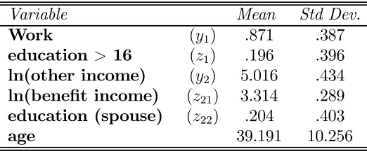
Table 4.1: Descriptive Statistics

Variable Mean Std Dev.

Work (y1) .871 .387

education > 16 (z1) .196 .396

ln(other income) (y2) 5.016 .434

ln(benefit income) (z21) 3.314 .289

education (spouse) (z22) .204 .403

age 39.191 10.256

Notes to Table 4.1:number of observations, 1606. The income and benefit

income variables are measured in log £’s per week. The education dummy (education>16) is a binary indicator that takes the value unity if the individual

stayed on a school after the minimum school leaving age of 16.

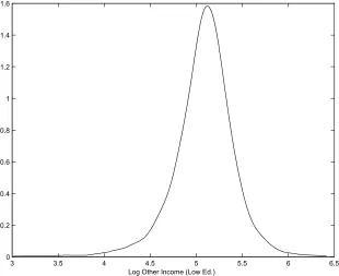
3 3.5 4 4.5 5 5.5 6 6.5 0

0.2 0.4 0.6 0.8 1 1.2 1.4 1.6

Log Other Income (Low Ed.)

Figure 1: Density of Log Other Income: Low Income Subsample

4.2. A Model of Participation in Work

To motivate the model specification, suppose that observed participation is described by a simple threshold model of labor supply. In this model the desired supply of hours of work for individuali can be written

h∗_i =δ0+z1iδ1+ lnwiδ2+ lnµiδ3+ζi, (4.1)

wherez1i includes various observable social demographic variables,lnwi is the log

hourly wage, lnµ_i is the log of ‘virtual’ other income, andζ_i is some unobservable heterogeneity. Aslnwi is unobserved for nonparticipants we replace it in (4.1) by

the wage equation

lnwi =θ0+z1iθ1+ωi (4.2)

wherez1i is now defined to include the education level for individual i as well as

other determinants of the market wage. Labor supply (4.1) becomes

h∗_i =φ₀+z1iφ1+ lnµiφ2 +νi. (4.3)

Participation in work occurs according to the binary indicator

y1i = 1{h∗i > h0i} (4.4)

where

h0i =γ0+z1iγ1+ξi (4.5)

is some measure of reservation or threshold hours of work.

Combining these equations, the binary response model for participation is now described by

y1i = 1{φ0+z1iφ1+ lnµiφ2+νi > γ0+z1iγ1+ξi} (4.6)

where y2i is the log other income variable (lnµi). This other income variable is

assumed to be determined by the reduced form

y2i = E[y2i|zi] +vi (4.8)

= Π(zi) +vi

andzi = [z1i,z2i].

In the empirical application we have already selected households by cohort, region and demographic structure. Consequently we are able to work with a fairly parsimonious specification in which z1i simply contains the education level

indicator. The excluded variables z2i contain the log benefit income variable

(denoted z21i)described above and the education level of the spouse (z22i).

4.3. Empirical Results

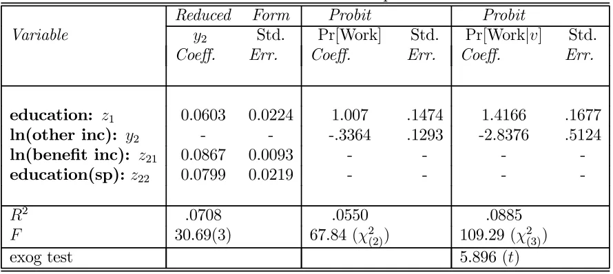
In Table 4.2 we present the empirical results for the joint normal (parametric) simultaneous probit model using the conditional likelihood approach, see (2.8). This consists of a linear reduced form for the log other income variable and a conditional Probit specification for the participation decision. Thefirst column of Table 4.2 presents the parametric reduced form estimates. Given the selection by region, cohort, demographic structure and time period, the reduced form simply contains the education variables and the log exogenous benefit income variable. The reduced form results show a strong role for the benefit income variable in the determination of other income.

significantly negative estimated coefficient on other income. The other income coefficient in Table 4.2 is the coefficient normalized by the education coefficient for comparability with the results from the semiparametric specification to be presented below.

As is evident from the results in the last columns of Table 4.2, the impact of adjusting for endogeneity is quite dramatic. The income coefficient is now considerably larger in magnitude and quite significant. The estimated education coefficient remains positive and significant. The asymptotic t-test for the null of exogeneity (see Blundell and Smith (1986)), strongly rejects the exogeneity of the log other income variable in this parametric binary response formulation of the labour market participation model.

Table 4.2: Results for the Parametric Specification.

Reduced Form Probit Probit

Variable y2 Std. Pr[Work] Std. Pr[Work|v] Std.

Coeff. Err. Coeff. Err. Coeff. Err.

education: z1 0.0603 0.0224 1.007 .1474 1.4166 .1677

ln(other inc): y2 - - -.3364 .1293 -2.8376 .5124

ln(benefit inc): z21 0.0867 0.0093 - - -

-education(sp):z22 0.0799 0.0219 - - -

-R2 _{.0708 .0550 .0885}

F 30.69(3) 67.84 (χ2₍₂₎) 109.29(χ2₍₃₎)

exog test 5.896(t)

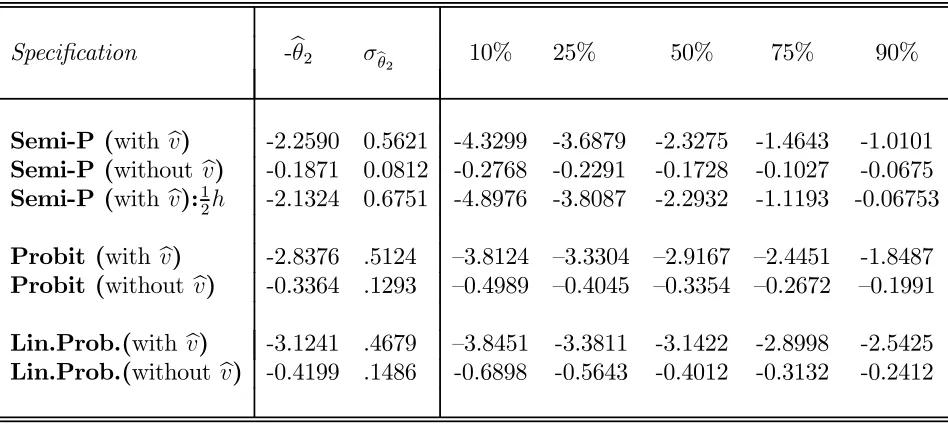
4.3 presents the estimation results for the β0 coefficients. The bootstrap

distri-bution relate to 500 bootstrap samples of size n ( =1606 ); the standard errors for the semiparametric methods are computed from a standardized interquartile range for the bootstrap distribution, and are calculated using the usual asymptotic formulae for the Probit and linear probability estimators.

The education coefficient in the binary response specification is normalized to unity and so the -θ2 estimates in Table 4.3 correspond to the ratio of estimates

of the other income coefficient to the education coefficient. In this application, bandwidths were chosen according to the 1.06σzn−

1

5 rule (see Silverman(1986)). These may well be too smooth for the estimation of β₀ and in the the third row we present results which use half this bandwidth (1₂h).This suggests the estimates are relatively robust for this sample over this range of this bandwidth.

For comparison, Table 4.3 presents results for the ratio of coefficients esti-mated assuming the errors are normally distributed (i.e., Probit, as in Table 4.2), as well as corresponding results from classical least squares and two-stage least squares (i.e., Linear Probability) estimators. The differing estimation methods yield qualitatively-similar conclusions concerning the endogeneity correction.

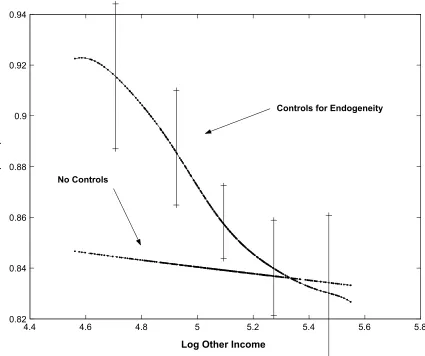
Figure 2 graphs the estimate of the average structural function ASF,G(xβ₀),

Table 4.3: Semiparametric Results and Bootstrap Distribution.

Specification -bθ2 σbθ2 10% 25% 50% 75% 90%

Semi-P (with _bv) -2.2590 0.5621 -4.3299 -3.6879 -2.3275 -1.4643 -1.0101

Semi-P (without _bv) -0.1871 0.0812 -0.2768 -0.2291 -0.1728 -0.1027 -0.0675

Semi-P (with _bv):1

2h -2.1324 0.6751 -4.8976 -3.8087 -2.2932 -1.1193 -0.06753

Probit (with _bv) -2.8376 .5124 —3.8124 —3.3304 —2.9167 —2.4451 -1.8487

Probit (without _bv) -0.3364 .1293 —0.4989 —0.4045 —0.3354 —0.2672 —0.1991

Lin.Prob.(with _bv) -3.1241 .4679 —3.8451 -3.3811 -3.1422 -2.8998 -2.5425

Lin.Prob.(without _bv) -0.4199 .1486 -0.6898 -0.5643 -0.4012 -0.3132 -0.2412

4.4 4.6 4.8 5 5.2 5.4 5.6 5.8 0.82

0.84 0.86 0.88 0.9 0.92 0.94

Log Other Income

P

ro

b

(

w

o

rk

)

Controls for Endogeneity

No Controls

Figure 2: Semiparametric regression with and without controls for endogeneity

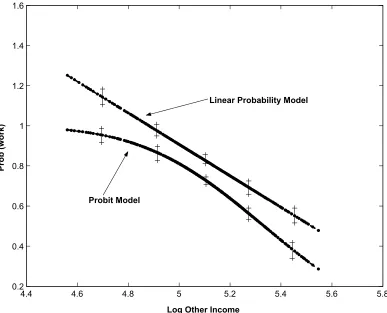
In Figure 3 we present corresponding results for the estimates of G(xβ0)

estimated β0 coefficients. Second, the proportion participating in the sample is

around 85% which suggests that the choice of probability model should matter as the tail probabilities in the Probit and linear probability models will behave quite differently. The plots show considerable sensitivity of the estimatedG(xβ₀),

4.4 4.6 4.8 5 5.2 5.4 5.6 5.8 0.2

0.4 0.6 0.8 1 1.2 1.4 1.6

Log Other Income

P

ro

b

(

w

o

rk

)

Linear Probability Model

Probit Model

Figure 3: Linear Probability and Probit Results with Endogeneity Controls

authors on request.

4.4 4.6 4.8 5 5.2 5.4 5.6 5.8

0.81 0.82 0.83 0.84 0.85 0.86 0.87 0.88 0.89

Log Other Income

P

ro

b

(

w

o

rk

)

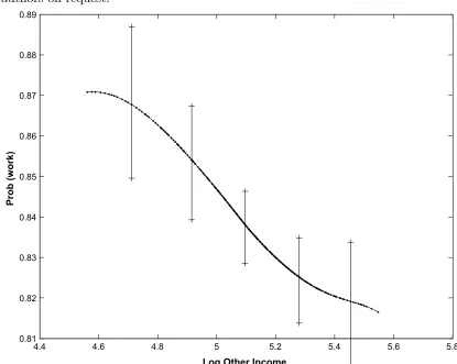
Figure 4: Nonparametric regression with controls for endogeneity

of the proposed estimator to an alternative representation of the simultaneous binary choice framework.

5. An Alternative Speci

fi

cation: Fixed Costs of Work and

The Coherency Model

One interpretation of the endogenous linear index binary response model de-scribed above is as the ‘triangular form’ of some underlying joint decision problem in terms of latent endogenous variables. Partitioning zas before

z= (z1,z2), (5.1)

we can express the model as

y1i = 1{y1∗i >0}, (5.2)

y∗_1i =z1iβ1+y2iβ2+ui (5.3)

and

y2i =z2iΞ1+y1∗iγ2+εi. (5.4)

Substitution of (5.3) in (5.4) delivers thefirst-stage regression model

y2i =ziΠ+vi (5.5)

for some coefficient matrixΠ.This ‘triangular’ structure hasy2 first being

deter-mined byz and the error terms v, while y1 is then determined by y2, z, and the

structural error u.

In this alternative specification (5.4) is replaced with a model incorporating feed-back between theobserved dependent variable y1 andy2

y2i =z2iΞ1+y1iα2+εi (5.6)

that is, the realization y1 = 1 results in a discrete shift y1iα2. Due to the

non-linearity in the binary response rule (5.2), there is no explicit reduced form for this system. Indeed, Heckman (1978), in his analysis of simultaneous models with dummy endogenous variables, shows that (5.2), (5.3) and (5.6) is only a statisti-cally ‘coherent’ system, i.e. one that processes a unique (if not explicit) reduced form, whenα2 =0, removing the direct feedback.

To provide a fully simultaneous system in terms of observed outcomes, and one that is also statistically coherent, Heckman (1978) suggests incorporating a structural jump in the equation fory∗1i,

y₁∗_i =y1iα1+z1iβ1+y2iβ2+ui, (5.7)

with the added restriction

α1+α02β2 = 0 (5.8)

This Heckman (1978) labels the Principal Assumption.9 _{Thus for a consistent}

probability model with general distributions for the unobservables and exogenous covariates we require the coherency condition (5.8). Below we show that the semi-parametric control function approach developed in this paper extends naturally

9_{To derive the condition (5.8) notice that from (5.2), (5.6) and (5.7)we can write}

y∗_1i= 1_{y∗_1i>0_}(α1+α2β2) +z1iβ1+z2iγ1β2+ui+εiβ2, (5.9)

or

to this framework. First we relate this coherency specification to a fixed costs model of participation.

Suppose that the fixed cost of work is given by α2. In determining

partici-pation, the fixed cost α2 will have to be subtracted from other income (or

con-sumption) for those who choose to work. In this case the model for other income

(y2i)will depend on the discrete employment decision(y1i),not the latent variable

(y1∗i). So that for those employment other income is defined net of fixed costs

e

y2i ≡y2i−y1iα2. (5.11)

The coherency restrictions (5.8) imply that (5.7) can be rewritten

y∗_1i = (y2i−y1iα2)β2+z1iβ1 +ui. (5.12)

The adjustment to y2i which guarantees statistical coherency is therefore

identi-cal to the correction to other income in the fixed cost model of labour market participation.

Definingy_e2i ≡y2i−y1iα2, the coherency condition implies that the model can

be rewritten

y1i = 1{z1iβ1+ye2iβ2+ui >0} (5.13)

and

e

y2i =z2iγ2+εi. (5.14)

If α2 were known then the equations (5.14) and (5.13) are analogous to (5.2),

(2.12) would be replaced by the modified conditional independence restrictions

u_|z1,y2,z2 ∼ u|z1,ey2, ε (5.15)

∼ u_|ε. (5.16)

The conditional expectation of the binary variable y1 given the regressors z1,ey2

and errorsε would then take the form

E[y1|z1,ye2i, ε] = Pr[−u≤z1iβ1+ey2iβ2|z1,ey2i, ε]

≡ F(z1iβ1+ey2iβ2, ε).

Finally, note that although α2 is unknown, given sufficient exclusion

restric-tions on z2i, a root-n consistent estimator for α2 can be recovered from (linear)

2SLS estimation of (5.6). More generally, if the linear form z2iγ1 of the

regres-sion function fory2 is replaced by a nonparametric formγ(z2i)for some unknown

(smooth) functionγ,then a√n-consistent estimator ofα2in the resulting partially

linear specification fory2i could be based on the estimation approach proposed by

Robinson (1988), using nonparametric estimators of instruments (z1i−E[z1i|z2i])

in an IV regression of y2i ony1i.

5.1. The Estimates of the Coherency Model

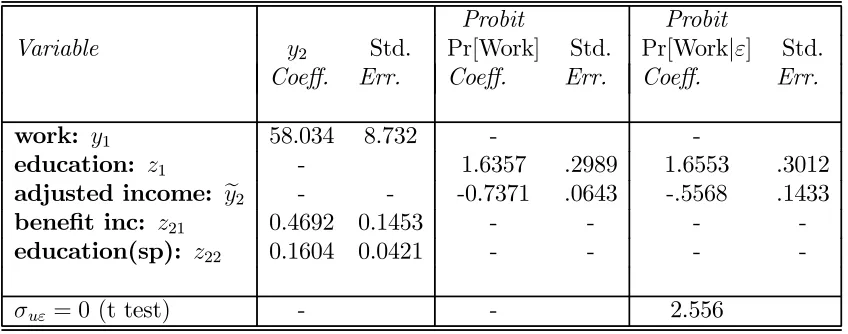
Thefirst column of Table 5.1 presents the estimates of the parameters of the structural equation for y2 (5.6). These are recovered from instrumental variables

ony2 through the adjustmentye2, there is much less evidence of endogeneity bias.

Indeed the coefficients on the adjusted other income variable in the two columns are quite similar (these are normalized relative to the education coefficient). If anything, after adjusting for fixed costs, controlling for endogeneity leads to a downward correction to the income coefficient.

Table 5.1: Results for the Coherency Specification.

Probit Probit

Variable y2 Std. Pr[Work] Std. Pr[Work|ε] Std.

Coeff. Err. Coeff. Err. Coeff. Err.

work: y1 58.034 8.732 -

-education: z1 - 1.6357 .2989 1.6553 .3012

adjusted income: y_e2 - - -0.7371 .0643 -.5568 .1433

benefit inc: z21 0.4692 0.1453 - - -

-education(sp): z22 0.1604 0.0421 - - -

80 100 120 140 160 180 200 220 240 260 0.83

0.84 0.85 0.86 0.87 0.88 0.89 0.9 0.91

Other Income

P

ro

b

(

w

o

rk

)

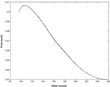
Figure 5: Semiparametric Estimation of the Coherency Model

Table 5.2: Semiparametric Results for the Coherency Specification.

Semi-P Semi-P

Variable Pr[Work] Std. Pr[Work_|ε] Std. Coeff. Err. Coeff. Err.

adjusted income: _ey2 -1.009 .0689 -0.82256 .2592

The comparable results for the semiparametric specification are presented in Table 5.2. In these we have used the linear structural model estimates for they2

a small difference in the other income coefficient between the specification that control forεand the one that does not. Again they_e2 adjustment seems to capture

much of the endogeneity between work and income in this coherency specification. In Figure 5 we present the semiparametric estimate of the probability of work across the whole low education sample. To evaluate this probability following the ASF formulation, used in the triangular specification, we have calculated y_e2 as if

each individual pays the fixed cost.

6. Summary and Conclusions

This paper has proposed and implemented a new semiparametric method for estimating binary response models with continuous endogenous regressors. The method introduces residuals from the reduced form as covariates in the binary re-sponse model to control for endogeneity. We considered a specific semiparametric “matching” estimator of the index coefficients which exploits both continuity and monotonicity implicit in the binary response model formulation. We have also shown how the partial mean estimator from the nonparametric regression litera-ture can be used to directly estimate the average structural function. The control function estimation approach, for this semiparametric model, is also shown to be easily adapted to the case where the model specification is not triangular and certain coherency conditions are required to be satisfied.

standard parametric models, the Probit and linear probability models, can give a highly misleading picture of the impact on participation of an exogenous change in other income.

References

[1] Ahn, H. (1995), “Non-parametric Two Stage Estimation of Conditional Choice Probabilities in a Binary Choice Model under Uncertainty,” Journal of Econometrics, 67, 337-378.

[2] Ahn, H. and J.L. Powell (1993), “Semiparametric Estimation of Censored Selection Models with a Nonparametric Selection Mechanism,” Journal of Econometrics, 58, 3-29.

[3] Ahn, H., Ichimura, H. and J.L. Powell (1996), “Simple Estimators for Monotone Index Models,” manuscript, Department of Economics, U.C. Berkeley.

[4] Amemiya, T. (1978), “The Estimation of a Simultaneous Equation Gener-alised Probit Model,” Econometrica, 46, 1193-1205.

[5] Blundell, R.W. and J.L. Powell (2003), “Endogeneity in Nonparametric and Semiparametric Regression Models,” in Dewatripont, M., L.P. Hansen, and S.J. Turnovsky, eds.,Advances in Economics and Econometrics: Theory and Applications, Eighth World Congress, Vol. II, Cambridge: Cambridge Uni-versity Press..

[6] Blundell, R.W., H. Reed and T. Stoker, (2003), “Interpreting Aggregate Wage Growth: The Role of Labour Market Participation”, American Economic Review,Vol. 93, No. 4, September, 1114-1131.

[8] Blundell, R.W. and R.J.Smith (1989), “Estimation in a Class of Simultaneous Equation Limited Dependent Variable Models”,Review of Economic Studies, 56, 37-58.

[9] Blundell, R.W. and Smith, R.J. (1994), “Coherency and Estimation in Simul-taneous Models with Censored or Qualitative Dependent Variables”,Journal of Econometrics, 64, 355-373.

[10] Das, M., W.K. Newey, and F. Vella (2003), “Nonparametric Estimation of Sample Selection Models,”Review of Economic Studies, 70(1), 33-58.

[11] Härdle W. (1990), Applied Nonparametric Regression, Cambridge: Cam-bridge University Press.

[12] Härdle, W. and T. Stoker (1989), “Investigating Smooth Multiple Regression by the Method of Average Derivatives,” Journal of the American Statistical Association, 84, 986-995.

[13] Heckman, J.J. (1978),“Dummy Endogenous Variable in a Simultaneous Equations System,”Econometrica, 46, 931-959.

[14] Honoré, B.E. and A. Lewbel (2002), “Semiparametric Binary Choice Panel Data Models Without Strictly Exogenous Regressors,” Econometrica, 70, 2053-2063.

[15] Hristache, M., A. Juditsky, and V. Spokoiny (2001), “Direct Estimation of the Index Coefficients in a Single Index Model,” Annals of Statistics, 29, 595-623.

[16] Ichimura, H. (1993), “Semiparametric Least Squares (SLS) and Weighted SLS Estimation of Single-Index Models,”Journal of Econometrics, 58, 71-120.

[17] Klein, R.W. and R.S. Spady (1993), “An Efficient Semiparametric Estimator of the Binary Response Model,”Econometrica, 61, 387-422.

[19] Lewbel, A. (2000), “Semiparametric Qualitative Response Model Estimation With Instrumental Variables and Unknown Heteroscedasticity,” Journal of Econometrics, 97, 145-177.

[20] Linton, O. and J.P. Nielson, (1995), “A Kernel Method of Estimating Non-parametric Structured Regression based on a Marginal Distribution,” Bio-metrika, 82, 93-100.

[21] Manski, C.F. (1975), “Maximum Score Estimation of the Stochastic Utility Model of Choice,”Journal of Econometrics, 3, 205-228.

[22] Manski, C.F. (1985), “Semiparametric Analysis of Discrete Response: As-ymptotic Properties of the Maximum Score Estimator,” Journal of Econo-metrics, 27, 205-228.

[23] Newey, W.K. (1994), “Kernel Estimation of Partial Means and a General Variance Estimator,”Econometric Theory, 10, 233-253.

[24] Newey, W.K., Powell, J.L. and Vella, F. (1999). “Nonparametric Estimation of Triangular Simultaneous Equations Models”, Econometrica, 67, 565-603.

[25] Powell, J., J. Stock and T. Stoker (1989), “Semiparametric Estimation of Index Coefficients,” Econometrica, 57, 1403-1430.

[26] Robinson, P.M. (1988), “Root n-Consistent Semiparametric Regression”, Econometrica, 56, 931-954.

[27] Silverman, B.W. (1986),Density Estimation for Statistics and Data Analysis, London: Chapman and Hall.

[28] Stock, J.H. (1989), “Nonparametric Policy Analysis,” Journal of the Ameri-can Statistical Association, 84, 567-575.