Measurement of drop size distribution time rate for liquid-liquid dispersion using IPI method

Measurement of drop size distribution time rate for liquid-liquid

dispersion using IPI method

Darina Jasikova1,*_{, Michal Kotek}1_{, Bohus Kysela}2_{, Radek Sulc}3_{, and Vaclav Kopecky}1

1_{Department of physical measurements, Institute for Nanomaterials, Advanced Technology and Innovation, Studentska 1402/2} 460 01 Liberec 1, Czech Republic

2_{Institute of Hydrodynamics AS CR, v. v. i., Pod Patankou 30/5, 166 12 Prague 6, Czech Republic}

3 _{Czech Technical University in Prague, Faculty of Mechanical Engineering, Department of Process Engineering, Technicka 4, 166 07} Prague, Czech Republic

Abstract. The liquid-liquid dispersion properties are studied mainly by image analysis (IA) and Interferometric Particle Imaging (IPI). Drop sizes will be investigated in dilute dispersion since in this case the break up phenomena is the dominating and is not affected by phase fraction. Characteristics of the size distribution and the evolution of two liquid-liquid phase’s disintegration were studied. The IPI method was used for subsequent detailed study of the disintegrated droplets. We compared two liquids: Rhodosil Oil 47V50, and Silicone Oil AP1000 under stirrer rate of 540 rpm, and 760 rpm. The experiment run in the scaled model of agitated tank with Rushton turbine.

1 Introduction

Mixing of liquids represents more than sixty percent of all industrial processes. A huge amount of mass is mixed in vessels stirred by an impeller. The global trend in process optimization involves new technologies providing higher quality products with lower energy demands. Trend is to develop more efficient mixing equipment.

Modern CFD methods are dealing with prediction of drop size distributions and their dynamics. This parameter determines mixing process evolution. The drop breakage, coalescence rates and final droplet size distribution depend on geometry of vessel and impeller, agitation rate and physical properties of mixed phases. Kolmogorov [1] and Hinze [2] were the first, who derived a relation for the maximum drop diameter. The maximum drop size dmax is determined by external deforming forces and restoration forces. [2]

The most mathematical descriptions and experimental studies focus on the characteristics of the process results, i.e. a steady dispersed system and final droplet size. Determination of this parameter is based on a collected small sample of the steady dispersed liquid. Many methods based on different physical principles are used to evaluate the stable dispersion. [3-5]

However, the course of the process, the temporal dependence of droplet size development is also important. The process dynamics is determined by the rate of disintegration of one phase. Tracking and evaluating the process is not a trivial problem. The requirement for the measurement method is the scanning frequency and sufficient time line. [5]

The motivation of our experimental work was to test the usability of an Interferometric Particle Imaging method (IPI) for recording and evaluating the course of liquid disintegration. The IPI method is suitable for measurement two-phase flows as well as liquid-liquid dispersion. [6-8]

2 Measurement Setup

Basically, measurement methods can be divided in two groups: the first one is based on sampling procedure; the second one is based on ex-situ measurements, i.e. capillary techniques. The overview of measurement techniques of drop size is in Bae (1989). As the inline methods are based on optical principles, the limiting factors are the size range and particle concentration.

The predicted size calculated using Weber equitation 𝑑𝑚𝑎𝑥 = 0.125. 𝑊𝑒−0.6. 𝐷 was 160 µm. Sauter mean diameter measured using high speed shadowgraphy from initial measurements was 120 µm. [1, 9] The maximal initial size of the disintegrated liquid is 500 µm. Knowing these edge limits, the IPI setup could be used.

The second limitation factor, the concentration, was estimated from the light scattering characteristics and the methodic of IPI technique. Backscatter technique allows a maximum concentration of 5% by volume. [5] The IPI method in principle can be expected to lower the limiting concentration of the liquid phase. Limit concentrations should be experimentally determined. [9]

Here we started with 1% of the liquid volume in agitated tank of the dispersed liquid phase.

2.1 Stirred Vessel Setup

We designed the scaled model of stirred vessel with inner diameter of cylindrical tank D = 150 mm and height H=D, position C = 1/4H.

We also used scaled model of Rushton turbine impeller of size D1 = 37 mm, w = 10 mm, l = 12 mm and t = 1 mm. The vessel was set with four baffles of width B/D=1/10, so was B = 15 mm fixed evenly around circumference of the vessel. The height of the liquid level was covered. The volume of water was 2.65 l.

There was used degassed water as a working liquid (density ρ = 1000 kg.m-3, viscosity μ = 1 mPa.s) under constant impeller speed 540 rpm and 760 rpm. The second liquid dispersed phase was Rhodosil Oil 47V50 (density ρ = 970 kg.m-3, viscosity υ = 50mm2/s, and surface tension  = 20. 7 mN/m), and Silicone Oil AP1000 (density ρ = 1009 kg.m-3, viscosity μ = 1000 mPa.s, and surface tension  = 40 mN/m) injected directly into the vessel. The volume of oil was set to 1% of liquid volume, so we used 26.5 ml.

Fig. 1. Geometry of stirred vessel, and a sketch of Rushton turbine impeller.

2.2 Interferometric Particle Imaging Method (IPI)

The interferometric method of droplet sizing or Interferometric Particle Imaging (IPI or ILIDS) can be attributed to the class of field optical investigation methods for two phase flows. One phase is liquid and second phase can be gas or liquid with different density, viscosity or immiscible liquid. It gives information about droplets in the whole chosen cross-section of the flow. That is great advantage of this method. The IPI can be apply to flow with lower densities of second phase and also requires optically transparent medium that enables light reflection and refraction.

The IPI was developed as the alternative to the Phase Doppler Anemometry (PDA). The IPI technique can provide instantaneous spatial distribution of particle diameter. The spatial pattern is generated by the interference of external reflection and direct refraction of the droplet that is placed in the laser sheet. The limits of this method are in the size of defocused image, when in denser systems particles interfere together. Deploying this method is appropriate when primary disintegration of liquid bulks has already occurred and disintegration of liquids leads to separated droplets in volume. This method gives results of long-term measurements for evaluation and validation final droplet size. It works very well on ranges of particle size (10 - 300) um. [6-8]

The IPI method uses the distance between the fringes of interference pattern which is formed by light reflected and once refracted by a droplet to measure the droplet diameter. The fringe pattern is created by defocusing of camera. The level of defocused particle image is between 50 px and 120 px. There are mathematical suggestions, but proper correction depends on actual scene, and light conditions. The measurement system is based on laser, formed in the light sheet, and digital camera with defocused lens. The camera registers interference patterns from all droplets illuminated by the light sheet. Here comes the restriction by droplet concentration.

Other limitations come with the physical background of IPI method. There are set lower and upper limits of measured particle diameter for each experimental setup. The first limit relates to geometrical optics. The second limitation depends on actual setup, i.e. camera distance, objective aperture, collecting angle. These limits are reflected in the number of interference fringes. The minimum number of fringes and therefore measurable diameter is N=2. Such a pattern can be easily created by secondary reflection. Evaluation of such noise as a valid particle is incorrect. This reading is reflected by shifting the peak to the smallest particles in the resulting histogram. Limits for maximal size of particles are related to Nyquist theorem. There is set the minimum distance between fringes in interference pattern x=2px. [8, 9, 10]

over the vessel diameter of size (160 x 135) mm. The laser sheet thickness was 3 mm, image was recorded on the camera HiSense Neo with resolution (2560x2160) px and 12-bit dynamic range. This camera was fitted with a lens with a focal length 60 mm (f/2.8). The distance between laser sheet and camera was 720 mm. This experimental setup with scattering angle 60° and aperture diameter of 15 enables measurement of droplet diameter from minimum 30 µm to maximum 457 µm.

We run IPI measurements on sampling frequency 2Hz. The camera’s external image buffer was able to capture only 258 records in each run. The long term measurement was separated into 3 runs. The first run was set immediately after the injection of oil into mixing process. Instantly started creation of large bulks of oil drops. Analysis of results contained image post processing procedures such as subtract of mean image to reduce scattered light, masking of objects and dark areas, and filters (edge detection, threshold). Stabile dispersion measurements were analysed for particle size distribution.

3 Results and Discussion

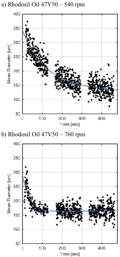
The experiment of two phases mixing was run for two stirrer speeds of 540 rpm and 760rpm. The scanned particle images were analysed by the pattern detection algorithm. Each record was evaluated for mean particle diameter (MPD) in the whole visualized area (i.e. the volume of the liquid where the volume coordinate is defined by the width of the laser plane, i.e. 3 mm, x and y are the vessel dimensions). There was obtained characteristic time dependence of the oil phase disintegration in the aqueous medium by evaluating the MPD at each time step (2 Hz). It was a sequence of 3 measurements in succession with a time delay, which is by downloading data from the external camera buffer into the computer memory as described in the limiting factors of the technique. MPD is characterized by value that can be roughly described as ±50 µm of MPD. The time dependence of MPD was interpolated by the equation power curve 𝑦 = 𝑎𝑥𝑏_{, where a, and b are} characteristic coefficient for each disintegration. The characteristic MPD is seen in Figure 2, and 3.

Table 1. Coefficients a and b for the interleaved time-dependent curve MPD

Rhodosil Oil 47V50 540RPM

Rhodosil Oil 47V50 760RPM

Silicone Oil AP1000 540RPM

Silicone Oil AP1000 760RPM

a 828.6 301.6 545.9 475

b -0.2936 -0.108 -0.2302 -0.192

A strong acceleration of the oil phase disintegration is characteristic at the beginning of the process from time coefficients a, and b. It is most significant for Rhodosil Oil 47V50 760 rpm. Our measurement lasted 10 minutes, to assume a complete steady state of disintegration, a mixing time of 25 minutes can be

expected. This time is calculated from the least accelerated dependences as a prediction.

a) Rhodosil Oil 47V50 – 540 rpm

b) Rhodosil Oil 47V50 – 760 rpm

Fig. 2. Mean Particle Diameter time dependence of Rhodosil Oil 47V50 for a) 540rpm, and b) 760 rpm stirrer speed.

Our goal was to assess the suitability of the IPI method for measuring the mixing process, as already mentioned in the introduction, therefore it does not matter much that we have not reached a fully steady state.

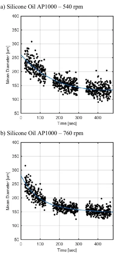
The evaluation of silicone oil blending appears to be disadvantageous for the higher rounds of the stirrer; however the variance of the measured MPD is lower (±30 µm). The comparison of interpolated curves is seen in Figure 4, and 5. These comparisons are more apparent but do not take into account the variations of the MPD measurements.

a) Silicone Oil AP1000 – 540 rpm

b) Silicone Oil AP1000 – 760 rpm

Fig. 3. Mean Particle Diameter time dependence of Silicon Oil AP1000 for a) 540rpm, and b) 760 rpm stirrer speed.

The last measurement interval, where we expected a more or less stable dispersion, was evaluated for the histogram of the oil phase particle size distribution. The largest size distribution was expected at a low mixing speed of Rhodosil Oil 47V50. If we start with knowledge of physical basis of disintegration process that is based on the ratio between viscous forces and Taylor theory of deformation generalized as Weber group, of condition, according to physical properties of Rhodosil Oil 47V50, its surface tension ratio is 𝑑 = 𝐾 (𝜌_𝜎)3/5𝜖−2/5_{. [10] This} equitation express the relation between final diameter and ratio between density  and surface tension , also taking in account local energy dissipation . The K is experimentally established constant. [11]

Fig. 4. Interpolated curves for Mean Particle Diameter time dependence of Rhodosil Oil 47V50.

Fig. 5. Interpolated curves for Mean Particle Diameter time dependence of Silicone Oil AP1000.

Similarly as for stable dispersions, the results of the IPI method can be used to evaluate histograms at each time point of the measurement. The overview of the distribution of the particles is the cumulative graphs (Fig. 7 and 8).

The comparison of cumulative number of drop size distributions shows significant change towards smaller particle size; when the stirrer rate is increased. The maximum drop size is a function of the energy input. The big difference is evident for Rhodosil Oil 47V50. We can also express different averages from these cumulative graphs, but this is already a question of interpretation.

Testing of the IPI system in a dynamic process brought important information. Validation measurements have also been performed. By evaluating more phases, at different mixing rates, the accuracy of the measurement and the methodology for the evaluation of the results were also confirmed. The IPI method can be used not only for the static processing of results, but also for tracking dynamic changes in the system with high

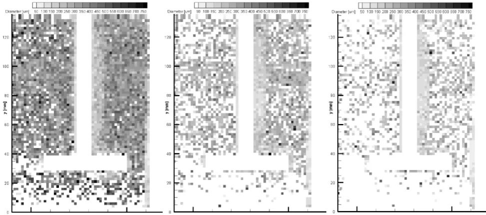
frequency. In this article, we have presented the results in the form of graphs, based on the principle of the IPI method, when the particles are measured in the entire area of interest, these results can also be processed graphically. The spatial distribution is seen in figure 9. This result corresponds with the methods of measurement that is seen in Fig. 2. The three runs that are separated due the time delay for data downloading are statistically processed with IPI spatial algorithm. The first result was calculated from the data between 0 sec and 130 sec; the second run between 170 sec and 300 sec and the third run between 340 sec and 470 sec. There is seen progress of disintegration of particles and their spatial distribution. The larger particles tend to be collected below the propeller. There are recirculation vortex structures in this area. It must be noticed, that the area just above the water tank bottom was not sufficiently illuminated with the laser sheet, so there is a lack of valid interferometric patterns. For this reason the size distribution's results does not represents the correct values - pretend to measure very small objects.

Fig. 7. Comparison of cumulative particle counts of stable dispersion of disintegrated Rhodosil Oil 47V50 under stirrer rate 540 rpm, and 760 rpm.

Fig. 8. Comparison of cumulative particle counts of stable dispersion of disintegrated Silicone Oil AP1000 under stirrer rate 540 rpm, and 760 rpm.

4 Conclusions

Here was proved that Interferometric Particle Imaging Method is suitable for detection of disintegration rate of liquid – liquid dispersions. The obtained data were analysed temporary in the size distribution statistics. These statistics interpolated with simple quotation express the time rate of disintegration. The method enables the expression of spatial distribution. The precise knowledge of these parameters help to improve and validate numerical simulation models of stirring process.

Authors gratefully thank to the support of Grant Agency of the Czech Republic (GA ČR) 16-20175S Local turbulent energy dissipation rate in dispersion systems, and LO1201 co-funding from the Ministry of Education, Youth and Sports as part of

targeted support from the „National Programme for Sustainability I".

References

1. A.N. Kolmogorov, Dokl.Akad.Nauk SSSR, 6 (1949) 2. J. O. Hinze, A.I.Ch.E. Journal, 1,3 (1955)

3. J. H.Bae, A.I.Ch.E. Journal, 35,7 (1989) 4. E.T. Hurlburt, Exp Fluids 32, 6 (2002) 5. S. Maaß, Exp Fluids 50, 2 (2011)

6. T. Kawaguchi, Meas. Sci. Technol., 13 (2002) 7. F. Pereira, Meas. Sci. Technol., 15 (2004) 8. Ch. Dunker, Meas. Sci. Technol., 27 (2016) 9. D. Jasikova, EPJ Web of Conferences, 180 (2018) 10. F. B. Sprow, Chem. Eng. Sci, 22 (1967)

11. C.A. Coulaloglou, AIChE Journal 22, 2 (1976) 12. K. Arai, J. Chem. Eng. Japan 10, 4 (1977)