OPE in Wilson lines with sub-eikonal spin corrections for TMDs and g1 structure function

OPE in Wilson lines with sub-eikonal spin corrections for TMDs

and

g

structure function

GiovanniAntonioChirilli1,*

1_{InstitutfürTheoretischePhysik,UniversityofRegensburg,D-93040Regensburg,Germany}

Abstract.Low-xevolution of spin-dependent TMDs and sping1 structure function are

relevant for the future Electron Ion Collider. To study spin-dynamics at high energies it is necessary to extend the eikonal approximation to include sub-eikonal corrections. I will discuss the Operator Product Expansion (OPE) in terms of Wilson lines with sub-eikonal corrections and derive the sub-eikonal quark propagator.

1 Introduction

Most of the progress in high-energy QCD has been obtained within the eikonal approximation. The high precision reached by the experiments and the possibility to study spin-dynamics in Deep Inelastic (DIS) scattering at the proposed Electron Ion Collider [1], makes the study of sub-eikonal corrections especially timely.

In order to access the sub-eikonal corrections in high-energy QCD one has to study the sub-eikonal corrections of the propagators of the theory extending, in this way, the Operator Product Expansion to include the sub-eikonal corrections. The result will be relevant for the study of TMDs andg1structure function.

In the eikonal approximation, the operator which describes the DIS scattering amplitude is a trace of two Wilson lines. Its evolution equation with respect to the rapidity of the fields gener-ates the Balitsky-hierarchy [3] which is equivalent to the Jalilian-Marian–Iancu–McLerran–Weigert– Leonidov–Kovner (JIMWLK) [6–8] evolution equation thus, they are referred to as B–JIMWLK equa-tion. The Balitsky-Kovchegov (BK) equation [4, 5] is the first of the Balitsky hierarchy and it is ob-tained in the mean field approximation. Its linearization coincides with the BFKL [9, 10] equation. As we will see, the sub-eikonal corrections will introduce new operators which we will result in new evolution equations thus providing further information on the QCD dynamics at high energy.

We will start with the derivation of the scalar propagator in the background of a highly boosted gluonic field generated by the target in order to lay down the formalism and the notation used. We then present the result for the quark propagator and make, as an example, a simple application of the OPE with the new derived operators.

2 Scalar propagator

2.1 Eikonal approximation

To reach the high-energy kinematics, we will perform a longitudinal boost of the fields generated by the target-particle in which the projectile particle propagates.

We assume that the projectile-particle is propagating alongp1direction, while the target particle is moving alongp2direction, wherep

µ

1andp

µ

2are two light-cone vectors such thatp1µp

µ

2 =p1·p2= s 2. We can perform a Sudakov decomposition of the momentum any momentumpµaspµ=αpµ₁+βpµ₂+

pµ_⊥. The light-cone components are defined as x_• = xµp µ

1 =

s

2x−and x∗ = xµp

µ

2 =

s

2x + _with

x±= x0√±x3 2 .

The gauge fieldAµ_{generated by the target, under a boost, gets rescaled by a large parameterλas}

follows

A_•(x_•,x_∗,x_⊥) → λA_•(λ−1x_•, λx_∗,x_⊥),

A_∗(x_•,x_∗,x_⊥) _→ λ−1A_∗(λ−1x_•, λx_∗,x_⊥), (1)

A_⊥(x_•,x_∗,x_⊥) _→ A_⊥(λ−1x_•, λx_∗,x_⊥).

In Schwinger representation the free scalar propagator is

�x_| i

p2_+iǫ|y�=i

d−4_ke−ik·(x−y)

p2_+iǫ , (2)

with�k_|x_�=eix·k. In (2) we used the_{-inspired notationd}−4_k≡ d4k

(2π)4 andδ−

(4)

(x₋y)=(2π)4δ(4)(x₋y) so that,d−4kδ−(4)(x₋y)=1.

In the eikonal approximation, the only component surviving the boost isA_•so, ˆP2 _≃pˆ2+2αgAˆ_• and we can represent the propagator as a series

�x_| i ˆ

P2_+iǫ|y� ≃ �x| i ˆ

p2_+iǫ|y�+g

d4z_�x_| i ˆ

p2_+iǫ|z�2iαA•(z∗,z⊥)�z| i ˆ

p2_+iǫ|y�+. . . . (3)

In the shock-wave picture (see Fig. 1) relevant for high-energy scattering, we assume that the particle starts and ends its propagation outside the interval in which the field strength tensor is different then zero (see Fig. 1). With this assumption we can rewrite expansion (3) as

�x_| i ˆ

P2_+iǫ|y�=

+_∞

0 d−_α

2αθ(x∗−y∗)−

0

−∞ d−_α

2αθ(y∗−x∗)

e−iα(x•−y•)

d2zd2z′_�x_⊥|e−i

ˆ

p2

⊥

αsx∗_|z ⊥�

×�z_⊥|Pexp

ig

x_∗

y∗

d2

sω∗e

iˆp2⊥

αsω∗_A •(ω∗)e−i

ˆ

p2_⊥

αsω∗

|z′_⊥��z′_⊥|eipˆ

2

⊥

αsy∗_|y

⊥�. (4)

Eq. (4) has been obtained assuming the commutation relation [ ˆα,Aˆ]=0 and the fact that the most dominant component of the gauge external field isA_•.

Under the longitudinal Lorentz boost, the longitudinal distance traveled by the particle in the external filed is rescaled asω_∗→ 1_λω_∗while the gauge field is rescaled asA_•→λA_•withλ_≫1 the boost parameter. So, we can write

ei

ˆ

p2_⊥

αsω∗_A •(ω∗)e−i

ˆ

p2_⊥

αsω∗_=A

Making use of (5) in propagator (4), we obtain

�x_| i ˆ

P2_+iǫ|y�=

+_∞

0 d−_α

2αθ(x∗−y∗)−

0

−∞ d−_α

2αθ(y∗−x∗)

e−iα(x•−y•)

×

d2z_�x_⊥|e−i

ˆ

p2

⊥

αsx∗_|z

⊥�[x∗, y∗]z�z⊥|ei

ˆ

p2

⊥

αsy∗_|y

⊥�, (6)

where we have defined the gauge link at fixed transverse positionz_⊥as

[x_∗, y_∗]z=Pexp

ig2

s x∗

y_∗

dω_∗A_•(ω_∗,z_⊥)

. (7)

Propagator (6) describes the propagation of the particle in the external field along a straight line. To consider deviation from the straight-line propagation we need to take into account higher order terms in Eq. (5).

Now we can trade the finite gauge link with the infinite Wilson line because, under the infinite boost, the dominant component of the field strength tensor,F_•i, has an infinitesimal thin support in x_∗coordinate and we assumed thatF_•iis peaked at the origin while outside the infinitesimal interval [₋ǫ_∗, ǫ_∗],F_•i=0 (see Fig. 1). Therefore, in the gauge rotated fieldAΩthe gauge field outside the ex-ternal field is zero and we can trade the gauge link [ǫ_∗,₋ǫ_∗] with the infinite Wilson line [_∞p1,−∞p1] and obtain

�x_| i

P2_+iǫ|y�=

+_∞

0 d−_α

2αθ(x∗−y∗)−

0

−∞ d−_α

2αθ(y∗−x∗)

e−iα(x•−y•)

×

d2z_�x_⊥|e−i

ˆ

p2

⊥

αsx∗_|z

⊥�Uz�z_⊥|ei

ˆ

p2

⊥

αsy∗_|y

⊥�, (8)

where we have defined the infinite Wilson lineUzat fixed transverse positionz_⊥as

Uz≡[p1∞,−p1∞]z=Pexp

ig2

s

+_∞

−∞

dz_∗A_•(2

sp1z∗+z⊥)

. (9)

Notice that, we can restoreAµ_⊥ component as a transverse gauge link (see Fig. 1) since it is a pure gauge.

2.2 sub-eikonal approximation

In this section we are interested in deriving the sub-eikonal corrections to the scalar propagator Eq. (6). To this end, we consider a background gauge field with all components different than zero, Acl

µ(x∗,x⊥)=(Acl∗(x∗,x⊥),Acl•(x∗,x⊥),Acl⊥(x∗,x⊥)), and we need to identify the most dominant compo-nent and sub-dominant one from the operator ˆP2_={pˆµ

⊥,Aˆ⊥µ}+{

2

sPˆ•,Aˆ∗} −gAˆ 2 ⊥.

It can be shown that the term_{2_sPˆ_•,Aˆ_∗}is related to the possibility for the fields to depend mildly on x_• but it contributes as sub-sub-correction, so we will neglect it and keep considering fields x_• independent.

It is convenient to define ˆO = _{pˆµ_⊥,Aˆ⊥_{µ} −}gAˆ2

⊥ so that ˆP2 = pˆ2 +2gαA•+gOˆ and the scalar propagator can be written as

�x_| i ˆ

P2_+iǫ|y�=�x|

i

ˆ

p2_+2αgAˆ

•+gOˆ+iǫ| y_�

=

+_∞

0 d−_α

2αθ(x∗−y∗)−

0

−∞ d−_α

2αθ(y∗−x∗)

e−iα(x•−y•)

×�x_⊥|e−i

ˆ

p2

⊥

αsx∗Pexp

ig

x∗

y_∗

d2

sω∗e

ipˆ2⊥

αsω∗

ˆ

A_•(ω_∗)+Oˆ(ω∗) 2α

e−i

ˆ

p2

⊥

αsω∗

ei

ˆ

p2

⊥

αsy∗|y

y_*

* *

x_{* z}

*

z

x

y

Figure 1.Particle propagating in an external gluonic field. The red strip represents the shock-wave defined in the infinitesimal interval [₋ǫ_∗, ǫ_∗] in whichFµν0. The light-red areas to the left and to the right of the shock-wave

represent the background filed made of pure gage field. The curvy line is the particle’s path from pointxto point y. The dotted lines represent the Wilson lines.

We are now ready to consider the sub-dominant contributions we neglected in the previous section. We observe that

ei

ˆ

p2_⊥

αsω∗

ˆ

A_•+ Oˆ

2α

e−i

ˆ

p2_⊥

αsω∗_=Aˆ •+

ˆ O 2α+i

ω_∗ αs[ ˆp

2

⊥,Aˆ•]+O(λ−1). (11)

Using Eq. (11), after some algebra we arrive at

�x_| i ˆ

P2_+iǫ|y�=

+_∞

0 d−_α

2αθ(x∗−y∗)−

0

−∞ d−_α

2αθ(y∗−x∗)

e−iα(x•−y•)

×�x_⊥|e−ipˆ

2

⊥

αsx∗

[x_∗, y_∗]+ ig 2α

₂

sx∗

{Pi,Ai(x_∗)_{} −}gAi(x∗)Ai(x∗)

[x_∗, y_∗]

−[x_∗, y_∗]2 sy∗

{Pi,Ai(y_∗)} −gAi(y_∗)Ai(y_∗)

+

x∗

y_∗

d2

sω∗

Pi,[x_∗, ω_∗]2

sω∗Fi•(ω∗) [ω∗, y∗]

+g

x_∗

ω_∗

d2

sω

′ ∗

2 s

_ω

∗−ω′∗

[x_∗, ω′_∗]Fi_•[ω_∗′, ω_∗]Fi_•[ω_∗, y_∗]

eipˆ

2

⊥

αsy∗_|y

⊥�+O(λ−2). (12)

As we will see in the next section, propagator (12) represent an intermediate useful step in order to obtain the quark propagator with sub-eikonal corrections.

3 Quark propagator with sub-eikonal corrections

The quark propagator in an external field in Schwinger notation is

�x_| i ˆ /

P+iǫ|y�=�x| ˆ /

P i

p2_+2αgA

•+gB+i2sgF•i/p2γi+iǫ

|y_� (13)

where we have definedB_≡O+ _s42gF_•∗σ_∗•+

g

2Fi jσ i j

To get the sub eikonal corrections to the quark propagator we have to expand (13) in terms of the sub-dominant contribution and repeat similar steps that we performed to get the sub-eikonal terms for the scalar propagator. Expanding we have

�x_|P/ˆ i

P2₊g

2Fµνσµν

|y_�=_�x_|P/ˆ i

P2 −

i

P2

_ig2 sFi•γ

i_/p

2+gB1 1 P2

+ i

P2

_ig2 sFi•γ

i /

p2+gB1

1 P2

_ig2 sFi•γ

i /

p2+gB1

1 P2

|y_� (14)

where we defined_B1= _s42F•∗σ∗•+

1 2σi jF

i j_.

We would like to obtain a gauge invariant expression of Eq. (14) so, after some algebra (see ref. [11] for the details of the derivation) we arrive at

�x_| i ˆ /

P+iǫ|y�=

+∞

0 d−α

2αθ(x∗−y∗)−

0

−∞ d−α

2αθ(y∗−x∗)

e−iα(x•−y•) 1 αs

×�x_⊥|e−i

ˆ

p2_⊥

αsx∗

ˆ /

pp/2[x∗, y∗] ˆp/+/pˆp/2Oˆ1(x∗, y∗;p⊥) ˆ/p

+pˆ/p/2 1

2Oˆ2(x∗, y∗;p⊥)− 1

2Oˆ2(x∗, y∗;p⊥)p/2p/ˆ

eipˆ

2

⊥

αsy∗_|y

⊥�+O(λ−2). (15)

where we have defined the operators

ˆ

O1(x_∗, y_∗;p_⊥)= ig 2α

x∗

y∗

d2

sω∗

[x_∗, ω_∗]1 2σ

i j_F

i j[ω∗, y∗]+pˆi,[x∗, ω∗] 2

sω∗Fi•(ω∗) [ω∗, y∗]

+g

x∗

ω∗

d2

sω

′ ∗

2 s

_ω

∗−ω′∗[x∗, ω′∗]Fi•[ω′∗, ω∗]Fi_•[ω_∗, y_∗]

, (16)

and

ˆ

O2(x∗, y∗;p⊥)= ig 2α

x∗

y∗

d2

sω∗

[x_∗, ω_∗]1

4(iDkFi j)

_σi j_{, γ}k

[ω_∗, y_∗]+

ˆ

pk,[x∗, ω∗]iFk jγj[ω∗, y∗]

+[x_∗, ω_∗]iFk jγj(iDk_[ω

∗, y∗])−(iDk[x∗, ω∗])iFk jγj[ω∗, y∗]

+( ˆα/p1−p/ˆ_⊥)[x∗, ω∗]i 2

sF•∗[ω∗, y∗]+(iD/⊥[x∗, ω∗])i 2

sF•∗[ω∗, y∗]

−[x_∗, ω_∗]i2

sF•∗(iD/⊥[ω∗, y∗])

, (17)

From propagator (15), given an observable in terms of operators, one may apply the high-energy OPE and obtain sub-eikonal corrections to the scattering amplitude as a convolution of coefficient functions and matrix elements of Wilson lines with the insertion of the new operators appearing in Eqs. (16) and (17).

4 OPE in Wilson lines with sub-eikonal corrections

for a review on Wilson lines formalism at high energy). For simplicity, let us consider only the sub-eikonal term given by the operator1₂Fi jσi j_{. We have}

�P,S_|ψ¯(x)γµψ(x) ¯ψ(y)γνψ(y)_|P,S_�x∗>=0>y∗

d2z1d2z2

tr_{X/1p/2Y/1γνY/2p/2X/2γµ} 4π6_x4

∗y4∗Z31Z 3 2

�P,S_|tr_{Uz1Uz†2}|P,S�

−g

d2z1d2z2

tr_{X/1p/2Y/1γνY/2p/2σi jX/2γµ} 64π6_x4

∗y4∗Z31Z 2 2

x∗

y∗ dω_∗

�P,S_|tr_{Uz1[−∞p1, ω∗]z2Fi j[ω∗,+∞p1]z2}|P,S�

+_�P,S_|tr{[+_∞p1, ω_∗]z2Fi j[ω∗,−∞p1]z2U

† z1}|P,S�

(18)

where we have defined

Zi≡

(x₋zi)2_⊥

x_∗ −

(y₋zi)2_⊥

y_∗ −

4

s(x•−y•) (19)

andXi≡x−zi, and Yi≡y−zi.

The first term after equal sign in Eq. (18) is given by the Leading Order (LO) Impact Factor (the coefficient function of an OPE), which has been known for more than 40 years, and matrix element of two Wilson lines whose evolution equation with respect to the rapidity parameter gives the BK equation [3–5] or the B-JIMWLK equation [6–8] according to whether we apply the mean-field approximation or not.

The second term after equal sign in Eq. (18) is the new term in the OPE which comes from the sub-eikonal corrections in the quark propagator. We would have more terms in OPE (18), had we considered all terms given in operators ˆO1and ˆO2.

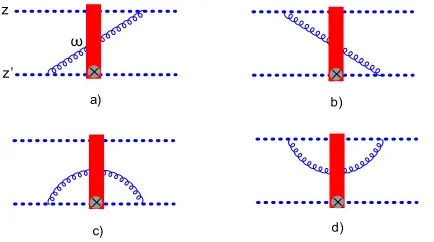
Let us consider the evolution equation of the Wilson line with the insertion of the operator1₂Fi jσi j. The one loop diagram are given in Fig. (2) and the evolution equation is

+_∞

−∞

dω_∗�tr_{[_∞,_−∞]z[−∞, ω_∗]z′gFi j(ω_∗)[ω_∗,∞]z′}�BK₋type

= αs 2π2

+_∞

−∞ dω_∗

+_∞

0

dα

α

d2ω (z−z

′₎2 ⊥ (z₋ω)2

⊥(z′−ω)2⊥

(20)

×tr{UzUω†}tr{Uω[−∞, ω_∗]z′gFi j(ω_∗,z′_⊥)[ω_∗,∞]z′} −Nctr{Uz[−∞, ω_∗]z′gFi j(ω_∗,z′_⊥)[ω_∗,∞]z′}

We observe that, besides the rapidity divergence given by₀∞d_αα we have an extra divergence for ω_→z′

⊥. The evolution equation (20) indeed, resum

αsln2 1_x B

, which is the type of resummation one finds in polarized DIS [12, 13].

5 Conclusions

We have presented the quark propagator with sub-eikonal corrections in high-energy QCD. Such result is relevant for the description, for example, of spin-dynamics at high-energy.

Most of the results obtained in the high-energy QCD have been obtained within the eikonal ap-proximation. Because of the high-precision reached by the experiments and the possibility to access spin-dynamics at the proposed Electron Ion Collider (EIC), the sub-eikonal corrections become rele-vant.

c) d)

a) b)

z

z’

Figure 2.BK-type diagrams for the operator give in Eq. (20)

As an example of the OPE with sub-eikonal corrections, we have considered the sub-eikonal correction described by the operator1₂Fi jσi j_{, and have obtained its evolution equation with respect to} the rapidity parameter. We noticed that, besides the usual rapidity divergence, which is related to the resummation ofαsln_x1

B, one has an extra divergence due to the presence of the operator 1 2Fi jσ

i j . This new divergence, together with the rapidity divergence, makes up the double Log divergence which is characteristic of the spin-dynamics at high energy.

References

[1] A. Accardi et al., Eur. Phys. J. A 52 (2016) no.9, 268 doi:10.1140/epja/i2016-16268-9 [arXiv:1212.1701 [nucl-ex]].

[2] I. Balitsky,“High-Energy QCD and Wilson Lines”, In *Shifman, M. (ed.): At the frontier of particle physics, vol. 2*, p. 1237-1342 (World Scientific, Singapore, 2001).

[3] I. Balitsky, Nucl. Phys. B463(1996) 99 doi:10.1016/0550-3213(95)00638-9.

[4] Y. V. Kovchegov,Small-x F2 structure function of a nucleus including multiple pomeron

ex-changes,Phys. Rev.D60(1999) 034008,

[5] Y. V. Kovchegov,Unitarization of the BFKL pomeron on a nucleus, Phys. Rev. D61 (2000) 074018,

[6] J. Jalilian-Marian, A. Kovner and H. Weigert, Phys. Rev. D 59, 014015 (1998) doi:10.1103/PhysRevD.59.014015 [hep-ph/9709432].

[7] J. Jalilian-Marian, A. Kovner, A. Leonidov and H. Weigert, Phys. Rev. D59, 014014 (1998) doi:10.1103/PhysRevD.59.014014 [hep-ph/9706377].

[8] E. Iancu, A. Leonidov and L. D. McLerran, Nucl. Phys. A692(2001) 583 doi:10.1016/ S0375-9474(01)00642-X [hep-ph/0011241].

[9] E. A. Kuraev, L. N. Lipatov and V. S. Fadin,The Pomeranchuk singlularity in non-Abelian gauge

theories,Sov. Phys. JETP45(1977) 199–204.

[10] I. Balitsky and L. Lipatov, The Pomeranchuk Singularity in Quantum Chromodynamics,

Sov.J.Nucl.Phys.28(1978) 822–829.

[11] G. A. Chirilli, arXiv:1807.11435 [hep-ph].

[12] J. Bartels, B. I. Ermolaev and M. G. Ryskin, Z. Phys. C70(1996) 273 [hep-ph/9507271]. [13] J. Bartels, B. I. Ermolaev and M. G. Ryskin, Z. Phys. C 72 (1996) 627