Metastable Q-balls
EminNugaev1,∗
1Institute for Nuclear Research of the Russian Academy of Sciences, 60th October Anniversary
Prospect 7a, Moscow 117312, Russia
Abstract.We will breifly review application of Euclidean path integral tech-nique for the study of quantum decay of the bound system in field theory with globalU(1)-invariance. As an illustration of the method, we numerically com-pute the decay rate of metastable Q-ball to the leading semiclassical order and present interpolating formula for the whole region of metastability.
1 Introduction
Theories with bosonic fields can provide extended lumps. These objects in models with sin-gle complex field are usually referred as Q-balls [1] or nontopological solitons in theories with additional fields [2]. Terminology indicates the crucial role of conserved nontopological chargeQwhich is determined by globalU(1)-invariance. Localization of charge and den-sity provided by nonlinear interaction and wealthy models usually considered only in small coupling regime. In this case properties of quantum state can be approximately described by solutions of classical fields equations with corresponding chargeQand energyE. Stability of configuration is not provided by topology of vacuum and we will assume that in the minimum of potentialV(0)=0 for value of complex field
ϕ=0. (1)
In quantum theory above the vacuum (1) complex field naturally results to bosons and antibosons with massm. It is natural to compare the energy of two configurations with the same chargeQ, i.e. soliton energyEand energy of free bosonsmQ1. In the case
E>mQ
the decay of soliton to free particles is kinematically possible. Examples with similarE(Q) dependence were provided by original model [3] of nontopological solitons and it is rea-sonable to calculate corresponding decay rate. Similar question considered in [4] for the modeling of trapped Bose-Einstein Condensate (BEC).
Although the metastable vacuum decay is thoroughly considered in [5], additional global U(1)-invariance provides some subtleties (see, for example [6]). There are also technical problems with exponential dependence of complex fields after Euclidean continuation. In the paper [7] we generalize the Coleman method and numerically calculate decay rate for a
∗e-mail: [email protected]
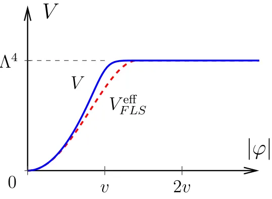
model with single complex field. The chosen scalar potential presented in Fig. 1 and the leading term ofVon smallest couplinggcan be expressed in the form
1
g2U(g|ϕ|/m).
Moreover, it can be used for description of dynamics of complex field in the
Friedberg-Lee-|
ϕ
|
V
Λ
4
0
v
2
v
V
F LS
eff
V
Figure 1.Scalar potential for numerical calculation.
Sirlin (FRS) model [3].
In this paper we will briefly review classical properties of Q-balls in the next section. In Sec. 3 we will discuss Euclidean equations of motion and main numerical results of [7].
2 Classical Q-balls
For a start, we briefly review the properties of smallQ-balls. To be concrete, consider the mode of complex scalar fieldϕwith potential
V=−m 2v2
b log
e−ϕϕ/v¯ 2+e−b
1+e−b
, b=8 (2)
shown in Fig. 1. The scalar bosons in this model have mass≈min vacuumϕ=0 and become almost massless at largeϕ:V →Λ4 ≡m2v2log(eb+1)/bas|ϕ| →+∞. This corresponds to short-range attractive interaction between the bosons.
Notably, the model possesses global conserved charge
Q=i
d3x(ϕ∂
tϕ¯−ϕ∂¯ tϕ) , (3)
The simplest way to find nontopological solitons in the model is to substitute stationary spherically-symmetric ansatz
ϕQ(x,t)=χQ(r) eiωt, r=|x|, (4)
into the classical field equations and numerically solve the resulting ordinary differential equation for realχQ(r) with regularity conditions∂rχQ(0)=χQ(∞)=0. Alternatively, one
can use piecewise parabolic function [8] to approximate potential and obtain a family of lo-calized solutions. Crucial for our study regimeE >mQcan be found for small Q-balls as it presented in Fig. 2.
Q
c
0
Q
s
Q
E
E
=
mQ
E
Q
(Q
)
decaying
Q
-balls
Figure 2.Metastable Q-balls forQc<Q<Qs.
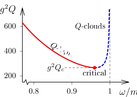
It should be noted that for the same chargeQone can obtain two solutions with different profiles, see Fig. 3. We will refer solution with smaller energy as Q-ball. There is additional branch of unstable solutions with larger energy and more widely profile — Q-clouds2. As pointed out in [10] Q-clouds can be interpreted as the critical bubbles between Q-balls and states with free particles.
Instability of Q-clouds corresponds to relativistic generalization of Vakhitov-Kolokolov criterion [11],∂Q/∂ω > 0. In Fig. 4 we presented crucial for this point dependenceQ(ω). The single mode of instability can be found in model with analytical solution [8, 10] or numerically [7]. Thus, Q-clouds mark the barrier between classically stable Q-balls and the state withQfree particles.
3 Euclidean method and results for the decay rate
For the false vacuum decay in models with real scalar fields there is powerful Euclidean tech-nique [5]. This process is described by the “bounce” — anO(4) invariant real Euclidean
1
2
4
8
|
ϕ
Q
|
/v
mr
0
Q
Q
Figure 3.Profiles of classical solutions for the same chargeQ.
200
400
600
0
.
8
0
.
9
1
ω/m
g
2
Q
Q
Q
g
2
Q
c
Figure 4.DependenceQ(ω) for Q-balls and Q-clouds. One can see that∂Q/∂ω >0 for Q-clouds.
solutionφcl(x2+τ2) coinciding with the false vacuum atτ→ −∞and arriving to the
catch-ment area of the true vacuum atτ=0. If continued to Minkowski timet≡ −iτ, this solution describes real field configuration, the bubble of true vacuum, evolving in the final state. The rate of false vacuum decay is exponentially suppressed, where the leading exponent is given by the Euclidean action of the bounceSE[φcl].
We expect to find similar, though properly modified, procedure for computing the rate of Q-ball decay. We should find semiclassical solutionϕcl(x, τ), ¯ϕcl(x, τ) satisfying Euclidean
field equations in the model,
(∂2
mr mτ
ρ(r, τ)
0 3 6 9
0
−20
−40
mr mτ
ρ(r, τ)
0 3 6 9
0
-40
-80
mr mτ
ρ(r, τ)
0 3 6 9
0 −80 −160 3v 2v v 0
ρ
(a) (b) (c)
Figure 5.Semiclassical solutionsρ(r, τ)≡(ϕϕ¯)1/2describing decay ofQ-balls withQ/Q
c≈1.05 (a),
1.33 (b), and 1.56 (c).
whereVis a derivative ofV( ¯ϕϕ) with respect to its argument. The boundary condition is
more subtle issue, see [7] for careful derivation. It is natural to expect that this solution coincides with theQ-ball (4) at the start of the process,
ϕcl→eωτ+η0/2χQ(r), ϕcl¯ →e−ωτ−η0/2χQ(r) as τ→ −∞, (6) where we introduced phase shiftη0of theQ-ball which cannot be excluded in general. It can
be represented in more appropriate for equations (5) form
ϕcl=e−ωβ−η0ϕcl¯ , ∂
τϕcl=−e−ωβ−η0∂τϕcl¯ at τ=−
β
2 → −∞,
which is consistent with the asymptotics (6). We should stress here that the functionsϕcland ¯
ϕclin Eq. (5) are not complex conjugate to each other. This situation is usual for the saddle point approximation. Our derivation suggests that instead of being mutually conjugate,ϕcl
and ¯ϕclcan be considered as independentrealfunctions ofxandτ. This gives real Euclidean action,
SE ≡ −iS =
β/2
−β/2dτd
3x∂
τϕ∂τϕ¯+∇xϕ∇xϕ¯+V(ϕϕ¯) , (7)
whereβwill be sent to infinity in the end of the calculation. Our second boundary condition ϕcl=ϕcl¯ , ∂τϕcl=−∂τϕcl¯ at τ=0 (8)
ensures that the solution describes classical evolution of waves/particles in the final state
after continuation to real time t ≡ iτ. Indeed, Eq. (8) implies that the functions ϕcl and ¯
ϕclare real and satisfyϕcl(x, τ)=ϕcl¯ (x,−τ) on the Euclidean time axis. This makes them
conjugate to each other at realt(imaginaryτ). Note that the solution can be continued to τ >0 usingτ → −τsymmetry. Numerically solving Eqs. (5) with corresponding boundary
conditions, one obtains a family of real solutionsϕcl, ¯ϕclinterpolating between theQ-ball (4)
and arriving to the sector of true vacuum atτ=0. In Euclidean time semiclassical solution
should to interpolate between localized soliton and homogeneous condensate as presented in Fig. 5 for different charges.
in:
Q
-ball
out: free particles
Q
Q
collective
tunneling
Figure 6.In final configuration of Q-ball decayϕ < v, i.e. the state is in the catchment of the vacuum.
Saddle-point approximation automatically provides result for the decay rate in the form
ΓQ=AQe−FQ
The main contribution to the suppression exponentFQcomes from classically forbidden
re-gion between Q-ball configuration and free particles atτ=0. Our result for the suppression exponent with its asymptotic and fitting function is presented in Fig. 7, quantitative expres-sions of them are:
FQ→d1+d2log (1−Q/Qs) , (9)
FQ≈(Q−Qc)c1+c2log (1−Q/Qs) , (10)
wherec1=−0.28,c2=−2.6.
0 2 4
1 1.2 1.4 Qs/Qc
F
Q/Q
c
Q/Q
cFQ
Fas
Q
FQf it
4 Conclusions
We developed general semiclassical method to calculate the decay rate ΓQ=AQe−FQ of
metastable Q-balls at Q 1. The method can be applied in arbitrary models at the cost of numerically obtaining certain Euclidean solutionsϕcl(x, τ) that enter the semiclassical
ex-pressions for the exponent FQand prefactor AQof the rate. We generalized the method to
finite-temperature processes.
To illustrate the method, we performed explicit numerical calculations in the model. Namely, we computed the exponent. Notably, the model we use is close to a certain limit of the celebrated Friedberg-Lee-Sirlin model [3] which describes complex and real fields with renormalizable potential.
Acknowledgments
I am indebted to A. Popescu for collaboration and especially to D. Levkov for collaboration and organization of the Seminar Quarks-2018. This work was supported by the Russian Science Foundation grant RSF 16-12-10-494.
References
[1] S. R. Coleman, Nucl. Phys. B262, 263 (1985) Erratum: [Nucl. Phys. B269, 744 (1986)]. [2] T. D. Lee and Y. Pang, Phys. Rept.221, 251 (1992).
[3] R. Friedberg, T. D. Lee and A. Sirlin, Phys. Rev. D13, 2739 (1976). [4] J. A. Freire and D. P. Arovas, Phys. Rev. A59(1999) 1461.
[5] S. R. Coleman, Phys. Rev. D15, 2929 (1977) Erratum: [Phys. Rev. D16, 1248 (1977)]. doi:10.1103/PhysRevD.15.2929, 10.1103/PhysRevD.16.1248
[6] K. M. Lee, Phys. Rev. D50, 5333 (1994)
[7] D. Levkov, E. Nugaev and A. Popescu, JHEP1712, 131 (2017)
[8] I. E. Gulamov, E. Y. Nugaev and M. N. Smolyakov, Phys. Rev. D87, no. 8, 085043 (2013)
[9] M. G. Alford, Nucl. Phys. B298, 323 (1988).
[10] E. Nugaev and A. Shkerin, Phys. Lett. B747, 287 (2015)