Difference Broadcast Encryption Scheme
Sanjay Bhattacherjee and Palash Sarkar Applied Statistics Unit
Indian Statistical Institute
203, B.T.Road, Kolkata, India - 700108.
{sanjayb r,palash}@isical.ac.in
Abstract
Broadcast Encryption (BE) is an important technique for digital rights management (DRM). Two key parameters of a BE scheme are the average size of the transmission overhead and the size of the secret information to be stored by the users. The most important BE scheme till date is the subset difference (SD) scheme proposed by Naor, Naor and Lotspiech in 2001 which achieves a good balance of these two parameters. A year later, Halevy and Shamir proposed a variant of the SD scheme called the layered SD (LSD) scheme which allowed to reduce the size of user storage at the cost of increasing the transmission overhead. Since then, there has been no further study of other possible trade-offs between transmission overhead and user storage that can be obtained from the SD scheme.
In this work, we introduce several simple ideas to obtain new layering strategies with different trade-offs between user storage and transmission overhead. At one end, we introduce the notion of storage minimal layering, show that the Halevy-Shamir layering does not achieve minimal storage and describe a dynamic programming algorithm to compute layering strategies for which user storage is guaranteed to be the minimum possible. This results in user storage being 18% to 24% lower than that required by Halevy-Shamir layering schemes. At the other end, we consider the constrained minimization problem and show how to obtain BE schemes whose transmission overhead is not much more than that of the SD scheme but, whose user storage is still significantly lower than that of the SD scheme.
The original SD and the LSD algorithms are defined only when the number of users is a power of two. In an earlier work, we have shown how to handle arbitrary number of users in the SD scheme. Here this is extended to the LSD scheme. Finally, we obtain anO(rlog2n) time algorithm to compute the average transmission overhead in any layering based SD scheme withnusers out of whichr are revoked.
Keywords: Broadcast encryption; subset difference; layering; transmission overhead; user storage
1
Introduction
Many real-life scenarios can be modelled as follows. There is a set of users and a centre which broadcasts messages. For each message, the centre decides on a set of users which should be able to access the message while the other users should not be able do so. The two subsets are respectively calledprivileged and revoked and they form a partition of the set of all users. A cryptographic system achieving such a functionality is called a broadcast encryption scheme [Ber91, FN93]. Practical applications include Pay-TV and more generally digital rights management.
A BE scheme can be based on symmetric key cryptography or on public key cryptography. In a symmetric key based BE scheme, the centre pre-distributes secret information to the users during a set-up phase. For a transmission, a session key is generated and the message is encrypted using the session key. Next the session key is encrypted using several other keys which are determined by the set of privileged users. The additional encryptions of the session key constitute theheaderwhile the actual encryption of the message is called thebody. To decrypt, a privileged user can use its secret information
to obtain one of the keys with which the session key has been encrypted. Decrypting the appropriate component of the header with this key yields the session key and then decrypting the body with the session key yields the message. The two important parameters of a BE scheme are the length of the header (as given by the number of encryptions of the session key) and the size of secret information to be stored by a user. It is desirable to decrease both as far as possible, but, in most schemes it turns out that decreasing one increases the other.
BE based on public key cryptography allows users to have public and private keys. There is no centre and anybody can encrypt to a subset of users. We do not consider public key BE in this work and instead refer the reader to relevant work such as [BF99, DF03, BGW05]. For this paper, by BE we will mean symmetric key BE.
Naor, Naor and Lotspiech (NNL) [NNL01] introduced an important BE scheme called the subset difference (SD) method. This scheme has been adopted as a standard for content protection in HD-DVD and Blu-ray discs [AAC]. The NNL-BE scheme is defined for nusers where nis a power of two, i.e., n= 2`0 for some `
0 ≥0. The users are considered to be the leaves of a full binary tree having `0
levels. Each user needs to store `0(`0+ 1)/2 k-bit strings where k is the key length of the underlying
symmetric key cryptosystem. Ifrusers are revoked, then the worst case header length (i.e., the number of encryptions of the session key) is 2r−1 [NNL01], while the average case header length turns out to be at most 1.25r for practical situations (see [BSar] for a detailed analysis). The trade-off between user storage and average header length turns out to be very well suited for real-life applications. Further, the scheme itself is quite elegant and reasonably easy to implement.
A later work by Halevy and Shamir [HS02] introduced a variant of the SD method called the layered subset difference (LSD) scheme. This is also defined for n users where n = 2`0. The basic idea is
to partition the tree into several layers which gives the name of the scheme. A different trade-off is obtained. User storage is reduced in the LSD method to `30/2−`0 but, the maximum possible header
length grows to 4r−3. In [HS02], based on simulation results, it is remarked that the average header length is around 2r. Compared to the SD method, the LSD method reduces the user storage at the cost of increasing the header length.
Our Contributions: We make a detailed analysis of the idea of layering introduced in [HS02]. It is
shown that the layering strategy introduced by Halevy and Shamir does not minimize the user storage. This is true for concrete values of n and asymptotically speaking the difference in the user storage between the HS layering strategy and a minimal storage layering strategy goes to infinity. In the HS layering strategy the root node of the user tree is treated as a special level. We show that by simply removing this condition yields a scheme where the user storage is `30/2 −`0 −(`0 −`10/2) and has a
negligible effect on the average header length. The notion of storage minimal layering is introduced. For such a layering strategy, user storage requirement is the minimum possible. An O(`30) time and
O(`2
0) space dynamic programming algorithm is presented to compute storage minimal layerings. The
resulting user storages are between 18% to 24% lower than that required by the Halevy-Shamir layering scheme.
Simply minimizing user storage is only one aspect of the problem. We consider the constrained minimization problem whereby one tries to minimize the user storage but, without increasing the average header length significantly beyond that achieved by the SD scheme. This is a difficult problem to solve analytically. Instead, we show how to tackle the problem empirically. Given some idea about the number of users that would be revoked, we show how one may use this information to design a layering strategy for which the average header length is almost as small as the SD scheme. The user storage for such a layering scheme is significantly less than that of the SD scheme. In fact, they are comparable to the LSD scheme storage requirements. Concrete practical examples are provided.
header length for the CTLSD scheme. Our study of the average header length of the CTLSD method as well as all experimental results have been computed using this algorithm.
Previous and Related Works: Subsequent to [NNL01, HS02], there have been some follow-up work
analyzing the average header lengths of the SD and LSD schemes. In [PB06], a generating function is obtained for counting the number of wayspusers out ofncan be given access privilege so that the header length will beh. For a givennandp, the generating function was used to obtain equations to compute the expected header length. The authors however mentioned that their equations were “complex to compute and difficult to gain insight from”. Consequently they went forward to findapproximationsfor the same. In contrast, our algorithm is efficient and simpler to implement. In [EOPR08] this analysis of the expected header length was continued and it was shown that the standard deviations are small compared to the expected values, as the number of users gets large. Other combinatorial studies of the SD method has been done in [MMW09, AK08]. All of these works considered the number of users to be a power of two. In [BSar], this condition was relaxed and the SD method was extended to the CTSD method. A detailed combinatorial and probabilistic analysis of the CTSD method was carried out.
Several works [LS98, PGM04] on the combinatorics behind broadcast encryption schemes and dif-ferent generic bounds on the efficiency parameters have been done. In [AKI03], a generic method for constructing BE schemes from pseudo-random generators was proposed. There have been several other works focussing on different aspects of BE [Sti97, SW98, GST04, AK08].
Several other BE schemes have been proposed. Linear algebraic techniques have been used in [PGMM03] to find a family of broadcast encryption schemes called linear broadcast encryption schemes. The same authors had also proposed key pre-distribution techniques based on linear algebraic techniques in [PGMM02]. Another interesting work on BE is [JHC+05], that works on the idea of “one key per punctured interval”. In [JHC+05], the worst case header length has been brought down to r or below for the first time, but at the cost of increasing user storage. But, the method is more complicated than the SD scheme and the user storage requirement is rather high.
A related and required aspect of BE schemes istraitor tracing [CFN94, FT01, NP98, KY01, SSW01], where pirate decryption boxes are used to trace the compromised keys. The traitor tracing method for the SD scheme can be modified to obtain a traitor tracing method for the CTLSD scheme and so we do not discuss this issue here.
2
Subset Cover Framework
Suppose there are n users. In the subset cover revocation framework, a collection S of subsets of
{1, . . . , n} is defined in a manner such that any set S ∈ S has an associated key and any subset of
{1, . . . , n} which is not inS does not have any key associated with it. For a useru, letSu ={S ∈ S : u∈S}. Useruis given secret informationIu such that it can construct the key associated with any set
inSu.
During the actual broadcast, some users are revoked and some are privileged. Suppose that a subset
T of the users are privileged. A cover finding algorithm determines a collection of pairwise disjoint subsets of S whose union isT. This collection of subsets is called the subset cover. The actual message is encrypted with a session key and the session key is encrypted with the keys associated with the subsets in the cover. The encrypted message forms the body while the different encryptions of the session key forms the header. So, the number of subsets in the cover determine the header length of the broadcast. Loosely speaking, this number itself is called the header length of the transmission.
To decrypt, a user first determines to which subset of the cover it belongs. Then, using its secret information, it generates the key associated with this subset. Decrypting the appropriate component of the header with this key, the user obtains the session key and then decrypting with the session key the user obtains the actual message.
also grows and this should lead to an increase in the size of Iu. Thus, the average header length and
the user storage are two competing parameters.
The Subset Difference Scheme. The SD scheme introduces a major novelty in defining S such
that there is a compact way of representing Iu. In the original SD scheme, the number of users n is a
power of 2, sayn= 2`0. Consider the users to be the leaves of a full binary tree. Each node in the tree
represents the users at the leaf level of the tree rooted at that node. Suppose iis a node of the tree and let S(i) denote the leaves of the subtree rooted ati. Let j be a node in the subtree rooted at i. Then
for the SD scheme, the setS consists of the subsetsS(i)\ S(j) for all possible choices of nodeiand all
possible nodes j6=iin the subtree rooted ati.
A clever algorithm is used to define the key associated with a setS(i)\ S(j). First each nodeiin the
tree is assigned an independent and uniform random labelLABELi. A cryptographically strong
pseudo-random generator (PRG) G:{0,1}k → {0,1}3k is used. Let G(seed) be written as the concatenation
of 3 k-bit strings GL(seed), GM(seed) andGR(seed). Suppose that a node j in the subtree rooted at
node iis reached from node i by the moves ‘left’, ‘left’ and ‘right’. Then the label of j derived from
LABELi is LABELi,j = GR(GL(GL(LABELi))) and the key associated with the set S(i) \ S(j) is
Li,j =GM(GR(GL(GL(LABELi)))).This easily extends to any appropriate pair of nodesiandj. The
stringLi,j is ak-bit string and the value ofkis determined by the key size of the underlying encryption
algorithm.
Recall that users are at the leaf level of the tree. The leaf level is numbered 0 and level numbers increase up to `0 which is the level number of the root. For any useru, the user storageIu is defined in
the following manner. Consider the path from the nodeuto the root and letibe a node on this path at level` >0 of the tree. Leti1, . . . , i` be the siblings of the nodes on the path fromutoi(includingubut
not including i). Then for each such i, user u gets the labelsLABELi,i1, LABELi,i2, . . . , LABELi,i`.
The value of ` varies from 0 to `0 and so each user gets `0(`0 + 1)/2 labels. The total size of Iu is
k`0(`0+ 1)/2 bits where k is the size of the seed of the PRG. Sincek is fixed, it is enough to consider
only the number of labels as determining the size of user storage.
The labels provided to a user is sufficient for the user to construct the key corresponding to any element in Su. To see this suppose that iis a node on the path from u to the root and j is a node in
the subtree rooted at i such that u ∈ S(i)\ S(j). Since u is not in S(j) and both u and j are in the
subtree rooted at i, the paths to root from these two nodes intersect for the first time at some node v
which is also in the subtree rooted at i. Let v1 be the first node in the path from v toj. Then v1 is
the sibling of some node v2 in the path from u to i and so u has LABELi,v1. From this label, u can
generateLABELi,j by applyingGLand GRappropriately and so can generateLi,j =GM(LABELi,j). This Li,j is the key corresponding to the setS(i)\ S(j). So,u can generate keys for any subset inS
u.
It is also required to argue thatucannot generate keys for any other subset inS. In the SD scheme, any subset in S is of the form S(i)\ S(j). Ifu is not in such a subset, then u is either not in S(i) or it
is inS(j). In either case, it is not too difficult to see thatudoes not obtain information which allows it
to generate Li,j. See [NNL01] for more details.
The Layered Subset Difference Scheme. The point of the LSD scheme is to reduce the user
storage in the SD scheme at the cost of increasing the header length. Reduction in the user storage is achieved by reducing the size ofS. As in the SD scheme, the LSD scheme also considers the number of users to be of the form 2`0 where the users form the leaves of a full binary tree. The major difference
between the SD and the LSD schemes is that in the LSD scheme the levels of the tree are partitioned into layers. Levels which form the boundary of the layers are called special levels.
A subsetS(i)\ S(j) is defined to be inS if either of the following two conditions hold:
• node iis at a special level;
• or, nodeiis not at a special level but, node j is in the same layer as level i.
This reduces the size ofS and consequently of Su. As a result, the size ofIu also reduces as we explain
i is a node at level ` in the path from u to the root and i1, . . . , i` are the siblings of the nodes in the
path fromutoi. If`is a special level, thenu is givenLABELi,i1, . . . , LABELi,i` as in the SD scheme.
Suppose`is not a special level. Let`0 be the first special level belowiand consider the segment of the path from u to iwhich lies between `0 and `. Suppose im, . . . , i` are the siblings of the nodes on this
segment. Thenugets LABELi,im, . . . , LABELi,i`. The net effect is that ifiis not at a special level, it
generates labels only up to the next special level. This leads to the reduction in the user storage. The reduction in user storage is achieved at an increase in the size of the header length. Suppose
i is not at a special level and j is in the sub-tree rooted at i but not in the same layer as i. The SD scheme would associate the set S(i)\ S(j) to such an (i, j) pair. In the LSD scheme, this set is not
present. Instead, the header computation algorithm will cover this set in the following manner. Let k
be the node in the first special level as one moves down the path from i toj. The sets S(i)\ S(k) and
S(k)\ S(j) are both present in the LSD scheme and it is easy to see that
S(i)\ S(j) =S(i)\ S(k) [ S(k)\ S(j).
This can be viewed as a two-way split of the setS(i)\ S(j). The work [HS02] also consider the possibility
of multi-way split. But, the authors conclude that this leads to further reduction in user storage only for impractical values of the number of users. In this paper, we will not consider multi-way split.
Halevy-Shamir (HS) Layering: In [HS02], the special layers are identified in the following manner.
Let d≤`0 be a fixed positive integer and write `0 =d(e−1) +p where 1≤ p≤ d. Then the special
levels are
`0,`0−d,`0−2d,. . .,`−d(e−1), 0.
So, there are a total of e+ 1 special levels and e layers out of which e−1 layers are of length deach and the last layer is of lengthp. Note thatpcan equaldwhich will lead toelayers each of lengthd. (If
p < d, then [HS02] does not consider the bottom-most level 0 to be a special level; notationally, we find it more convenient to always have level 0 as a special level and this does not have any effect on either the user storage or the header length.)
In [HS02], the suggested value ofdis √
`0
. By the Halevy-Shamir (HS) layering strategy we will mean the strategy with layer lengths d, d, . . . , d, pwithd=√`0
.
3
General Layering Strategy
We analyze the LSD scheme where the layer lengths are not necessarily equal. Suppose there are (e+ 1) special levels and the numbers of the special levels are`0> `1 > ... > `e−1 > `e= 0.Let`= (`0, . . . , `e).
The user storage for such a strategy can be calculated as follows. Corresponding to each special level `i, a user has to store `i labels. Now consider the nodes in the layer bordered by `i and `i+1.
Corresponding to any non-special level j in this layer a user has to store j−`i+1 labels. So, the total
number of labels that is required to be stored by a user considering both special and non-special levels is given by the following formula.
storage0(`) =
e−1
X
i=0
`i+ e−1
X
i=0
`i−1
X
j=`i+1+1
(j−`i+1)
=
e−1
X
i=0
`i+
e−1
X
i=0
`i−`i+1−1
X
j=1
j
=
e−1
X
i=0
`i+
1 2
e−1
X
i=0
(`i−`i+1)(`i−`i+1−1). (1)
It is sometimes more convenient to use another formulation. For 1 ≤ i ≤ e, define di = `i−1 −`i
d = (d1, . . . , de) whose sum is `0, it is possible to define a layering scheme where `i = `0−Pij=1dj.
Using (1) we have the following.
storage0(`) = `0(e+ 1)−
e
X
i=1
(e−i+ 1)di+
1 2
e
X
i=1
di(di−1). (2)
Some consequences of (1) and (2) are mentioned below.
1. If all the di’s are equal to d and `0 =e×d, then storage0(`) is given by `0(e+d)/2−`0. This
shows that the user storage using e layers of length deach is the same as the user storage using
d layers of length e each. If all the layer lengths are equal, then the problem of minimizing the user storage is that of minimizing the sume+dsubject to the constrainted=`0. From this it is
easy to see that the minimum value is attained for e =d=√`0 and the corresponding value of
user storage is`30/2−`0. Since,`0 may not be a perfect square one may takedto be
√
`0
. This justifies the choice made in [HS02]. Note that the minimization here is in the context of all the layer lengths being equal.
2. If each di equals 1, then each level is a special level and the resulting scheme becomes identical to the SD scheme. Similarly, if e= 1, i.e., only the root and the leaf levels are the special levels, then also the resulting scheme is the SD scheme. In both the cases the expression given by (2) is maximized and the value is`0(`0+ 1)/2.
3. Let d = (d1, . . . , de), d0 = (d1, . . . , de−1,1, . . . ,1
| {z }
de
) and suppose ` and `0 are the corresponding
layering strategies. Then the labels stored by a useruare the same for both cases and consequently,
storage0(`) = storage0(`0). In other words, at the end, having a single layer of length de is the
same as having de layers of length 1 each.
4. Suppose d = (d1, . . . , de) with d1 ≥ d2 ≥ · · · ≥ de and d0 = (dπ(1), . . . , dπ(e)) where π is a
permutation of {1, . . . , e}. Let ` and `0 be the corresponding sequences of special levels. Then
storage0(`)≤storage0(`0). This can be seen by noting that the quantity`0(e+1) and the quadratic
terms in (2) are the same in both cases. A simple argument then shows the required inequality. As an example, suppose `0 = 12 and fix e = 8. Then the scheme having (d1, d2, . . . , d8) =
(2,2,2,2,1,1,1,1) requires a storage of 50 labels whereas the scheme having (d1, d2, . . . , d8) =
(1,1,1,1,2,2,2,2) requires a storage of 66 labels.
5. Consider the HS layering strategy where `0 = d(e−1) + p with 1 ≤ p ≤ d and d =
√
`0
. Then d = (d, . . . , d
| {z }
e−1
, p). Since p can be much less than d one can consider a strategy where
the layer lengths are balanced. Write `0 = d(e−1) +p = (e−d+p)d+ (d−p)(d−1) and
define d0 = (d, . . . , d
| {z }
e−d+p
, d−1, . . . , d−1
| {z }
d−p
). Let ` and `0 be the corresponding sequences of special
levels. Then, one can show that storage0(`) = storage0(`0). Experimental results show that the average header lengths for both strategies are similar with that corresponding to `0 being slightly smaller. As an example, for `0 = 18, d0 = (5,5,4,4) yields lesser expected header lengths than
d = (5,5,5,3) for all r between 256 and 16384 while the user storage 75 is the same for both. These expected header lengths are computed using the algorithm (described later) for computing average header length.
6. Letd= (d1, . . . , de) and suppose thatdi =d+δandde−j+1 =d, i.e., the i-th entry from the front
isd+δ and thej-th entry from the end isd. Suppose that d0 is obtained fromd by incrementing
di(i.e., changing its value to d+δ+ 1) and decrementingde−j+1(i.e., changing its value tod−1).
Let ` and `0 be the corresponding sequences of special levels. A simple calculation based on (2) shows that storage0(`)−storage0(`0) = (e−i−j−δ).So, if e > i+j+δ, then it is possible to reduce storage by incrementingdi and decrementingde−j+1. This simple observation can be used
to show that the HS layering strategy does not minimize the storage requirement. Letd=√`0
and assume that d divides `0 such that `0 = d×e. (If d does not divide `0, then it is easy to
modify the argument below.) Then the HS layering scheme will bed= (d, d, . . . , d). Letθ≥1 be such thate >2θ and define
d0= (d+ 1, . . . , d+ 1
| {z }
θ
, d, . . . , d, d−1, . . . , d−1
| {z }
θ
).
Thenstorage0(`) =storage0(`0) +θ(e−θ−1). The gapθ(e−θ−1) is positive. In fact, as`0 goes to
infinity,ealso goes to infinity and the gap goes to infinity. This, however, does not imply that the layering strategy from d0 provides the minimum storage. There could be other more non-uniform layering strategies which further reduce the storage requirement.
Root as a non-special level: In [HS02], the root level `0 is always taken as a special level. It is
possible to obtain further reduction in user storage if we allow the root level to be a non-special level. Having the root as a special level contributes `0 labels to the user storage. If instead the root is made
a non-special level, then its contribution to the user storage will be `0−`1 labels. Given a sequence of
level numbers `, let storage1(`) be the number of labels required to be stored when the root is not a special level (and so, `1 is the first special level). Then the following relation holds.
storage1(`) = storage0(`)−`1. (3)
Equivalently,
storage1(`0, . . . , `e) =
(`0−`1)(`0−`1+ 1)
2 +storage0(`1, . . . , `e). (4) So, not having the root to be a special level reduces the storage requirement by `1 labels. This can be
quite significant. Consider the HS layering strategy where `0 =d×eand so `= (`0, `1, . . . , `e) where `i−`i+1 =dfor 0≤i < e. In this case, storage0(`) =`
3/2
0 −`0 andstorage1(`) =` 3/2
0 −`0−(`0−`10/2).
Given a layering strategy`= (`0, . . . , `e), there are e+ 1 special levels irrespective of whether the
root is a special level or not. If the root is a special level, then there areelayers and if the root is not a special level, then there aree+ 1 layers with the top layer having only one special level at the bottom. It is important to understand the effect on the header length when the root level is not special. During the computation of the cover, suppose that the root generates an SD subset, i.e., the SD cover finding algorithm returns a subset of the form S(0)\ S(j). Since the root is not at a special level, this
subset may be split into two ifj is not in the first layer. We argue that for reasonable values of r (the number of revoked users), this effect is negligible. In fact, the argument is that the probability of the root generating an SD subset itself is small.
The root generates an SD subset only if exactly one of the two subtrees of the root node contains all the revoked users. Suppose the revoked users are uniformly distributed, i.e., r users are uniformly sampled one-by-one without replacement and revoked. Then the probability that the left subtree does not have any revoked user (and consequently the right subtree contains all of them) is
1−n/2
n 1−
n/2
n−1
· · ·
1− n/2 n−r+ 1
=
1−1
2
1− 1
2 1−1
n
!
1− 1
2 1− 2
n
!
· · · 1− 1
2 1−r−1
n
!
3.1 Storage Minimal Layering
For a given value of `0, let SML0(`0) denote a layering strategy ` (or equivalently is given by the
sequence of differences d) including the root level, such that storage0(`) takes the minimum value among all possible layering strategies for a tree with`0 levels. Let #SML0(`0) denotestorage0(`) where
` is a storage minimal layering strategy. Similarly define SML1(`0) and #SML1(`0) that exclude the
root level from being special.
We describe a dynamic programming based algorithm to compute SML0(`0) (and subsequently
SML1(`0)). The idea of the algorithm is explained as follows. For a fixed value of `0, the number of
layersecan vary from 1 to`0. The casese= 1 ande=`0 correspond to the SD scheme and in these two
cases the user storage is known to be equal to `0(`0+ 1)/2. Let SML0(e, `0) denote a storage minimal
layering using exactlye layers. Clearly, the following relation holds.
#SML0(`0) = min 1≤e≤`0
#SML0(e, `0). (5)
Also,
#SML0(e, `0) = min (`0,...,`e)
storage0(`0, `1, . . . , `e) (6)
where the minimum is over all possible layering strategies (`0, `1, . . . , `e). The following relation is
obtained from (1).
storage0(`0, `1, . . . , `e) = `0+`1+· · ·+`e+
(`0−`1)(`0−`1−1)
2
+(`1−`2)(`1−`2−1)
2 +· · ·+
(`e−1−`e)(`e−1−`e−1)
2
= `0+
(`0−`1)(`0−`1−1)
2 +storage0(`1, . . . , `e). (7) Consequently,
#SML0(e, `0) = min 1≤`1<`0
`0+
(`0−`1)(`0−`1−1)
2 + #SML0(e−1, `1)
. (8)
This relation is the basis for the algorithm. Let Tab be an `0 ×`0 table such that Tab[e][`0] =
#SML0(e, `0). A simple O(`30) time dynamic programming algorithm can fill up this table as follows.
for`= 1,2, . . . , `0,
Tab[1][`] =Tab[`][`] =`(`+ 1)/2; for`= 1,2, . . . , `0,
fore= 2,3. . . , `0−1,
Tab[e][`] = min1≤`1<`(`+ (`−`1)(`−`1−1)/2 +Tab[e−1][`1]).
Using (5) provides #SML0(`0) as the minimum value in column number`0 of Tab. Note that the
minimum may occur for more than one possible value ofe. These values of `1 are reported during the
computation. Let Λ(e, `0) be the list of all possible values of`1 for which (8) holds. The above method
can be extended to generate all possible layering strategies for which user storage is minimized. An SML0 layering strategy`can be generated as follows. Start with`as the list containing only`0
and keep on appending in the following manner to obtain the complete sequence. Let e be one of the possibilities for whichTab[e][`0] takes the minimum value; choose `1 as any one value from Λ(e, `0) and
append to`; choose`2 as any one value from Λ(e−1, `1) and append to`; continue until 0 is appended
to the list. All SML0 strategies can be generated by looping over all possible values of e, all possible
values of `1, all possible values of `2 and so on.
OnceTab is prepared, computing #SML1(`0) using (4) is easy.
#SML1(`0) = min
e min`1
#SML0(e−1, `1) +
(`0−`1)(`0−`1+ 1)
2
(9)
= min
e min`1
Tab[e−1][`1] +
(`0−`1)(`0−`1+ 1)
2
Table 1: Comparison of user storage and expected header lengths between HS-LSD and SML. The tuples contain header lengths normalized with the SD header lengths corresponding to the values of r
in (rmin, . . . , rmax) respectively.
`0 rmin rmax scheme special levels storage normalized header lengths for (rmin, . . . , rmax)
12 22 28
SD 12,0 78 (1.00,1.00,1.00,1.00,1.00,1.00,1.00,1.00,1.00,1.00) HS 12,8,4,0 42 (1.69, 1.57,1.53,1.45,1.38,1.31,1.26,1.22,1.18,1.15) SML0 12,8,5,3,1,0 40 (1.68, 1.54,1.53,1.49,1.46,1.44,1.43,1.42,1.42,1.42) SML1 8,5,3,1,0 32 (1.68, 1.54,1.53,1.49,1.46,1.44,1.43,1.42,1.42,1.42)
16 26 212
SD 16,0 136 (1.00,1.00,1.00,1.00,1.00,1.00,1.00,1.00,1.00,1.00) HS 16,12,8,4,0 64 (1.66, 1.57,1.53,1.45,1.38,1.31,1.26,1.22,1.18,1.15) SML0 16,11,7,4,2,0 61 (1.64, 1.53,1.53,1.52,1.50,1.47,1.44,1.42,1.39,1.38) SML1 11,7,4,2,0 50 (1.64, 1.53,1.53,1.52,1.50,1.47,1.44,1.42,1.39,1.38)
20 28 214
SD 20,0 210 (1.00,1.00,1.00,1.00,1.00,1.00,1.00,1.00,1.00,1.00) HS 20,15,10,5,0 90 (1.68,1.64, 1.64, 1.60,1.55,1.50,1.45,1.41,1.38,1.34) SML0 20,14,9,6,3,1,0 85 (1.71,1.56, 1.57, 1.58,1.58,1.57,1.56,1.55,1.54,1.54) SML1 15,10,6,3,1,0 70 (1.68,1.64,1.65,1.63,1.60,1.58,1.56,1.55,1.55,1.54)
24 210 216
SD 24,0 300 (1.00,1.00,1.00,1.00,1.00,1.00,1.00,1.00,1.00,1.00) HS 24,19,14,9,4,0 116 (1.63,1.68, 1.63, 1.61, 1.61, 1.61, 1.62, 1.62, 1.63, 1.64) SML0 24,18,12,7,3,1,0 112 (1.63,1.65, 1.61, 1.58, 1.56, 1.56, 1.56, 1.56, 1.57, 1.57) SML1 18,12,8,5,3,1,0 94 (1.68,1.64,1.65,1.63,1.60, 1.58, 1.57, 1.56, 1.55, 1.54)
28 210 216
SD 28,0 406 (1.00,1.00,1.00,1.00,1.00,1.00,1.00,1.00,1.00,1.00) HS 28,22,16,10,4,0 146 (1.69,1.70, 1.75, 1.75, 1.74, 1.73, 1.72, 1.71, 1.70, 1.69) HS0 28,22,16,10,5,0 146 (1.69,1.70,1.75,1.75,1.74,1.73,1.71, 1.70, 1.69, 1.68) SML0 28,21,15,10,6,3,1,0 140 (1.74,1.63, 1.67, 1.71, 1.72, 1.72, 1.71, 1.70, 1.69, 1.68) SML1 22,16,11,7,4,2,0 119 (1.69,1.68, 1.72, 1.71, 1.69, 1.67, 1.66, 1.64, 1.63, 1.63)
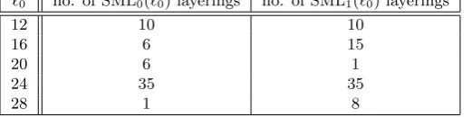
Table 2: The number of SML0(`0) and SML1(`0) layering strategies for various values of`0.
`0 no. of SML0(`0) layerings no. of SML1(`0) layerings
12 10 10
16 6 15
20 6 1
24 35 35
28 1 8
The first minimization is over the number of layers and the second minimization is over the value of the first special level. The possible corresponding layering strategies can also be easily recovered. It is to be noted that the SML1(`0) layerings are due to the minimization of the user storage by assuming the
root to be at a non-special level. It can be seen from (8) and (9) that in an SML0(`0) layering, if the
root is made non-special, it might not necessarily result in an SML1(`0) layering and vice versa.
Table 1 shows values of user storage for SML strategies for some`0. For comparison, we also show
the storage requirements for the SD scheme and the HS layering strategy. Compared to the SD scheme, the HS layering strategy reduces the storage requirement very significantly. Compared to the HS scheme the value of #SML0(`0) is slightly smaller and the value of #SML1(`0) is about 18% to 24% lower for
the newly suggested values of `. So, given a value of `0, if the requirement is to minimize the user
storage, then the SML strategies offer better alternatives. They also guarantee that further lowering of storage cannot be achieved by 2-way splitting of SD subsets.
The effect of SML0(`0) and SML1(`0) strategies on the average header length is also shown in Table 1.
For computing the average header lengths, we have considered ten values of r equally spaced between
rmin and rmax. The reported values are the average header lengths of the different schemes normalized
by the average header length of the SD scheme. As an example, the first value 1.69 corresponding to the row for HS and `0= 28 means that with n= 228 users out of whichr= 210 are uniformly revoked,
the average header length of the HS layering strategy is 1.69 times that of the SD scheme.
Table 3: List of SML0(`0) and SML1(`0) layering strategies denoted by the special levels for `0 = 12.
10 Special levels for SML0(12) 10 Special levels for SML1(12)
12,7,4,2,1,0 8,4,2,1,0
12,8,4,2,1,0 8,5,2,1,0
12,8,5,2,1,0 8,5,3,1,0
12,8,5,3,1,0 9,5,2,1,0
12,7,3,1,0 9,5,3,1,0
12,7,4,1,0 9,6,3,1,0
12,7,4,2,0 8,4,1,0
12,8,4,1,0 8,4,2,0
12,8,4,2,0 8,5,2,0
12,8,5,2,0 9,5,2,0
1. For a fixed `0, there may be more than one SML0(`0) (resp. SML1(`0)) strategy which achieves
storage of #SML0(`0) (resp. #SML1(`0)). Table 2 gives the number of SML strategies for several
values of `0. For `0 = 12, Table 3 lists all possible SML0(`0) and SML1(`0) strategies. There,
however, need not be a single layering strategy which minimizes expected header length for all possible values of r. Out of these, one would be interested in the layering that would give the minimum expected header length for most values of r under consideration. The SML strategies reported in Table 1 have this feature.
2. For`0= 32, Tabhas been computed and reported in Table 7 in the Appendix. It gives the values
of the minimum storage for every 1 ≤`0 ≤32 and 1≤e≤`0. For a particular `0 and e, it also
gives the values of `1 for which (8) holds. As an example, we see that for `0 = 32 and e = 8,
#SML0(e, `0) = 172 and the values of `1 are 24 and 25. All possible SML0(`0) strategies for
1 ≤ `0 ≤ 32 can be obtained from this table and the SML1(`0) strategies can subsequently be
found using (9).
3. As discussed earlier, if the root level is made non-special in an SML0 strategy, it may not lead to
an SML1 strategy and vice versa. Table 3 shows that while the SML0 strategy`= (12,8,4,2,1,0)
gives rise to an SML1 strategy ` = (8,4,2,1,0) by making the root level non-special, the SML0
strategy `= (12,7,4,2,1,0) does not. On the other hand, the SML1 strategy `= (9,5,2,1,0) is
not generated from an SML0 strategy.
4. Extensive experiments have shown that for practical values of r, there is no significant difference between the average header lengths of SML0 and SML1strategies that differ at only the root being
at a special level or not. For`0= 12 and 16, the reported SML0 strategy with the root level made
non-special turns out to be an SML1 strategy (as reported in Table 1) with minimum expected
header lengths. This supports the theoretical justification described before. However, for`0= 20,
it turns out that making the root level of the SML0 strategy non-special does not give rise to an
SML1 strategy. For `0 = 24 and 28, it is again true that making the root level of the reported
SML0 strategy non-special gives rise to an SML1 strategy. But there are other SML1 strategies
that further reduce the expected header lengths and hence we report those strategies in Table 1.
5. For `0 = 28, the HS layering strategy marks the levels 28, 22, 16, 10, 4, 0 as special. Halevy and
Shamir [HS02] also consider an alternative layering strategy where the levels 28, 22, 16, 10, 5, 0 are made special. We have denoted this by HS0 and reported the average header lengths for this in Table 1.
6. In general, the header length of the HS scheme is smaller than that of SML0 and SML1. This is
somewhat expected, since user storage in SML is smaller. On the other hand, the user storage is not the only determining factor. The actual layering strategy also plays a role and in some cases the average header length in SML is smaller than that in HS. As a result, in such cases, we see that bothuser storage and average header length are reduced. These are marked in bold and are particularly noticeable for `0 = 24 and `0 = 28. In the context of AACS standard [AAC], SML1
3.2 Constrained Minimization of User Storage
From the viewpoint of minimizing communication bandwidth it is of interest to minimize the average header length. This is minimized when the number of keys is maximized which happens for the SD scheme, i.e., when all the levels are considered to be special levels or there is only a single layer. Taking the average header length for the SD scheme as a benchmark, one may ask the question as to how much the user storage can be reduced from that required by the SD scheme without significantly increasing the average header length. The expression for the average header length (as can be derived from (11), (13) and Proposition 2 given later) is rather complicated and it appears quite impossible to have an analytical solution to this question. Instead, we use our average header length computation program to study this behaviour. It turns out that it is indeed possible to significantly reduce the user storage with minimal increase in the average header length.
It has been earlier mentioned that the probability of the root generating an SD subset is small. We build on this intuition. Suppose there are n users and r of them are revoked. In [BSar] it has been shown that the probability that a particular node at level `generates a subset in the header is
2(ηr(n,2`−1)−ηr(n,2×2`−1)−ηr(n,3×2`−1) +ηr(n,4×2`−1))
whereηr(n, x) = (1−x/n)(1−x/(n−1))· · ·(1−x/(n−r+ 1)) ifn > r−1 else 0. Since there are 2`0−`
nodes at level`, the expected number of subsets arising from all nodes at level `is
2`0−`(ηr(n,2`−1)−ηr(n,2×2`−1)−ηr(n,3×2`−1) +ηr(n,4×2`−1)). (10)
For a fixed n and r, one can consider the problem of finding ` such that this quantity is maximized. One can then make level `special. This will ensure that the subsets generated from this level will not be split due to the layering scheme. Avoiding the splitting of a large number of subsets will have a mitigating effect on the overall header length.
To be able to carry out this strategy, we need to find` for which (10) is maximized. Analytically, this seems to be very difficult to do. Instead we have done extensive experimentation. Empirical values suggest that the maximum occurs for some level `≤`0− blog2rc. Also, for` > `0− blog2rc, the value
of (10) is quite small.
Based on this empirical evidence we suggest the following layering strategy.
• Make`0− blog2rc special.
• No level ` < `0− blog2rc is made special. In terms of user storage and expected header length
this is equivalent to making all levels` < `0− blog2rc to be special.
• The root level is not made special.
• At most one level that is midway between `0 and `0− blog2rc is made special. While this does
not significantly affect header size, it can reduce the storage requirement.
This strategy will ensure that if`≤`0− blog2rc, then no SD subset generated from level`will be split.
One issue with this strategy is that the value ofrwill not be known a priori while the layering scheme will have to be decided upon during the design phase itself. A way out is to make an assumption about the minimum number of revoked users that will occur in the steady state operation of the BE scheme. For example, in AACS with 228users one may assume that in the steady state at least 210 users will be revoked due to data piracy problems.
Suppose thatrmin is the minimum number of users that will be revoked during each broadcast. The
above layering strategy is used withrmin. Suppose now that during a broadcast, the number of usersr
that is actually revoked is greater than rmin. Then from our empirical evidence the level for which the
average header length is maximized will be `0− blog2rc. Since this value is less than `0− blog2rminc,
none of the subsets generated from this level will be split. So, the feature of not splitting a large number of SD subsets is still retained.
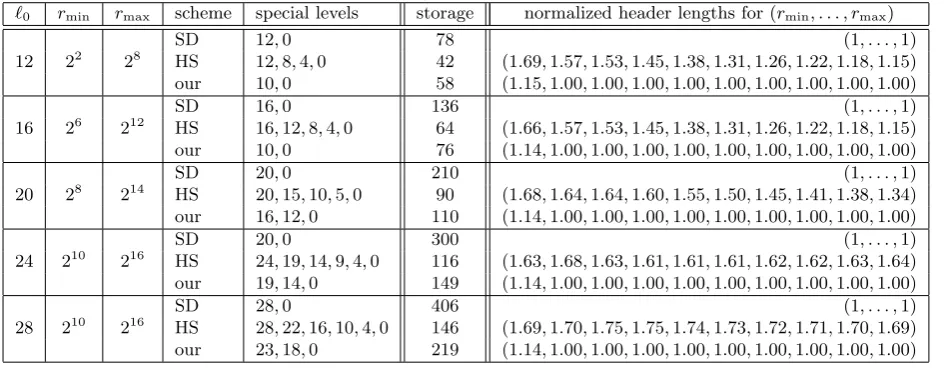
Table 4: Comparison of user storage and average header length for SD, HS-LSD and our constrained minimization layering. The tuples contain header lengths normalized with the SD header lengths cor-responding to the values of r in (rmin, . . . , rmax) respectively.
`0 rmin rmax scheme special levels storage normalized header lengths for (rmin, . . . , rmax)
12 22 28
SD 12,0 78 (1, . . . ,1)
HS 12,8,4,0 42 (1.69,1.57,1.53,1.45,1.38,1.31,1.26,1.22,1.18,1.15) our 10,0 58 (1.15,1.00,1.00,1.00,1.00,1.00,1.00,1.00,1.00,1.00)
16 26 212
SD 16,0 136 (1, . . . ,1)
HS 16,12,8,4,0 64 (1.66,1.57,1.53,1.45,1.38,1.31,1.26,1.22,1.18,1.15) our 10,0 76 (1.14,1.00,1.00,1.00,1.00,1.00,1.00,1.00,1.00,1.00)
20 28 214
SD 20,0 210 (1, . . . ,1)
HS 20,15,10,5,0 90 (1.68,1.64,1.64,1.60,1.55,1.50,1.45,1.41,1.38,1.34) our 16,12,0 110 (1.14,1.00,1.00,1.00,1.00,1.00,1.00,1.00,1.00,1.00)
24 210 216
SD 20,0 300 (1, . . . ,1)
HS 24,19,14,9,4,0 116 (1.63,1.68,1.63,1.61,1.61,1.61,1.62,1.62,1.63,1.64) our 19,14,0 149 (1.14,1.00,1.00,1.00,1.00,1.00,1.00,1.00,1.00,1.00)
28 210 216
SD 28,0 406 (1, . . . ,1)
HS 28,22,16,10,4,0 146 (1.69,1.70,1.75,1.75,1.74,1.73,1.72,1.71,1.70,1.69) our 23,18,0 219 (1.14,1.00,1.00,1.00,1.00,1.00,1.00,1.00,1.00,1.00)
the expected header length normalized with respect to the SD scheme. The average header length depends on the number r of revoked users. So, for a given n= 2`0, we computed the expected header
lengths for 10 equispaced values of r between and including rmin and rmax. The values in the table
illustrate the point that compared to the SD scheme, the constrained minimization layering schemes substantially reduce the user storage with a small increase in the average header length.
The layering scheme is designed assuming that the number of revoked users is at leastrmin. What
happens if the number of revoked users in an actual broadcast is smaller than rmin? Clearly, we cannot
expect the average header length to still be almost equal to that of the SD scheme. This effect is shown for some values ofr in Table 5. Again the values of the average header length are normalized by that of the corresponding SD scheme. For comparison, we have also provided the average header lengths of the HS layering strategy. It is to be noted that the expected header lengths of the new schemes are mostly better than the HS scheme. As an example, for n= 224, forr >6, our strategy gives smaller expected header lengths than the HS layering strategy. Table 5 shows that for any value of n, the new layering strategies lead to smaller expected header lengths for allr >15.
To summarize, the constrained minimization layering strategy gives low expected header length if
r ≥rmin. Ifr < rmin, then it is better than HS layering but inferior to the SD scheme. It is to be noted
that if r is small, then the absolute size of the header itself is not too large. As a result, the effective transmission overhead of the scheme will never be too high compared to the actual body of the message.
3.3 Tackling Arbitrary Number of Users
In [NNL01] and [HS02], the number of users have been taken to be a power of two, i.e.,n= 2`0. This is
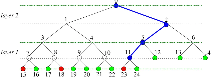
not always convenient as has been argued in details in [BSar]. By modifying the structure of the tree, it is possible to handle arbitrary number of users. This modification is based on the notion of complete binary trees. These are trees where the leaf nodes are at most two different levels and the last level has all its nodes to the left side. An example of a complete subtree accommodating 13 users is shown in Figure 1. In this case `0 = 4 and choosing d= 2 gives two layers and three special levels as shown in
the figure. When the number of users is a power of two, the corresponding tree is called a full binary tree. This difference in terminology between full and complete has been taken from the literature on data structures.
We explain some terminology with respect to Figure 1. The left and the right subtrees of node 3 are the subtrees rooted at nodes 7 and 8 respectively. The sibling subtree of node 3 is the subtree rooted at node 4. The only non-full subtrees are those rooted at nodes 0, 2 and 5. We call the path labelled by the nodes 0, 2, 5 and 11 to be thedividing path.
Table 5: Comparison of average header length for r < rmin between HS layering strategy and the
constrained minimization layering strategy.
`0 rmin scheme special levels storage header lengths normalized with the SD scheme
12 22
r= (1,2,3,4) HS 12,8,4,0 42 (1.00,1.74,1.72,1.69)
our 10,0 58 (2.00,1.50,1.26,1.15)
16 26
r= (2,4,6,8,10,12,14,16,18,20) HS 12,8,4,0 64 (1.75,1.70,1.66,1.63,1.61,1.60,1.60,1.60,1.60,1.61) our 10,0 76 (1.78,1.74,1.70,1.66,1.63,1.59,1.56,1.53,1.50,1.47) 20 28
r= (2,4,6,8,10,12,14,16,18,20) HS 20,15,10,5,0 90 (1.77,1.75,1.72,1.70,1.68,1.66,1.65,1.64,1.63,1.63) our 16,12,0 110 (1.77,1.69,1.64,1.61,1.59,1.57,1.56,1.56,1.56,1.56) 24 210
r= (2,4,6,8,10,12,14,16,18,20) HS 24,19,14,9,4,0 116 (1.77,1.75,1.72,1.70,1.68,1.66,1.65,1.64,1.63,1.63) our 19,14,0 149 (1.79,1.75,1.72,1.69,1.67,1.65,1.64,1.63,1.62,1.61) 28 210
r= (2,4,6,8,10,12,14,16,18,20) HS 28,22,16,10,4,0 146 (1.79,1.78,1.76,1.74,1.73,1.72,1.71,1.70,1.69,1.68) our 23,18,0 219 (1.79,1.75,1.72,1.69,1.67,1.65,1.64,1.63,1.62,1.61)
a complete binary tree with n leaves and having the root node at level `0. The leaves and hence,
the users are at either levels 0 or 1. Suppose the layering sequence is ` = (`0, . . . , `e) For users at
level 0, the storage requirement is storage0(`) while for users at level 1, the storage requirement is
storage(`)−(e+p−2) wherepis the number of levels in the bottom-most layer. This reduction is due to the fact that these users need to store one less label for each special level above it and for each level in its last layer. The distribution of labels using the PRG is done as usual.
1 2
6
10
7 14
5 4
3
15 16 17 18 19 20 21 22 23 24
11 12 13
9 8
0
layer 2
layer 1
Figure 1: A complete subtree with 13 leaf nodes.
During a broadcast, the actual header generation is done in much the same way. First, as in the SD scheme, the set of non-revoked users is covered exactly by subsets of the formSi\ Sj whereiis a node
in the tree and j is a node in the subtree rooted ati. If i is at a non-special level and j is not in the same layer as i, then this set is further split into S(i)\ S(k)
∪ S(k)\ S(j)
where k is the first node appearing at a special level on the path from itoj.
Complications for complete but non-full trees arise due to the following reason. For some internal nodes, the subtree rooted at it may not be full. All such nodes lie on the dividing path. A node not on the dividing path and at level`is the root of a subtree having either 2` leaves or 2`−1 leaves accordingly as whether the node is to the left or to the right of the dividing path. As an example, in Figure 1, nodes 3, 4, 5 and 6 are at level 2. Node 5 is on the dividing path and the subtree rooted at node 5 is non-full; nodes 3 and 4 are to the left of 5 and are the roots of subtrees having 22= 4 leaves; node 6 is to the right of node 5 and the subtree rooted at 6 has 2 leaves.
SD scheme by reducing the user storage at the cost of almost double the transmission overhead. The CTLSD scheme provides the best trade-offs between the user storage and the transmission overhead for practical values of r. The transmission overhead is almost as good as the (CT)SD scheme, while the user storage is reduced to almost half of it. This is demonstrated at the end of Section 4 using Table 6.
4
Header Length
The main point of the discussion in this section is to obtain an efficient algorithm for computing the expected header length for the CTLSD scheme and hence the LSD scheme. But, before that we state the following bound on the worst case header length.
Proposition 1. The maximum header length in the CTLSD scheme for n users out of which r are
revoked is min (4r−2,n2, n−r).
Proof. The bound is independent of the actual layering strategy. The upper bound of 2r−1 for the SD scheme was already given in [NNL01] and in [BSar] it was shown that this also holds for the CTSD scheme. Using the layering strategy, each subset returned by the SD algorithm can split into at most two subsets. So, if the number of SD subsets is at most 2r−1, then there are at most 4r−2 subsets.
Suppose the header consists of h subsets out of which h1 are singleton sets and h2 sets have 2 or
more elements each. For each node in a singleton privileged set, its sibling (if there is one) must be a revoked user. Among all these leaves, there is only one which may not have a sibling that is also a leaf node (and this is the first privileged user from the left at level 1, for odd n). So, for the h1 privileged
users, there are at leasth1−1 other revoked users. This accounts for at leasth1+h1−1 + 2h2 = 2h−1
users. It is now easy to argue that ifh >dn/2e, then 2h−1 is greater than n. Since the total number users is n, this cannot happen. Soh≤ dn/2e.
Since each subset in the subset cover will have at least one privileged user, the maximum number of subsets in the header is equal to the number of non-revoked users which is equal to n−r.
The bound of 4r−2 holds for both the cases when the root is or is not a special level. If the root is a special level the bound of 4r−2 can be improved to 4r−3. We first provide a short argument to justify that in the SD scheme if the header length is 2r−1, then there is a subset of the form S0\ Sj
in the header. As mentioned earlier, such a subset is added to the header if and only if exactly one of the subtrees of the root node do not contain any revoked user. So, if such a subset is not in the header, then both the subtrees of the root node contain at least one revoked user. Suppose the number of revoked users in these two subtrees are r1 and r2 where r = r1+r2. Applying the bound on the
maximum header length, we have the header to be of maximum length 2r1−1 + 2r2−1 = 2r−2. So,
if the header length is 2r−1, then there must be a subset of the type S0\ Sj in the header. Using the
layering strategy, each subset returned by the SD algorithm can split into at most two subsets. So, if the number of SD subsets is at most 2r−2, then there are at most 4r−4 subsets. On the other hand, if the number of SD subsets is equal to 2r−1, then as argued above there must an SD subset of the form S0\ Sj in the header. Since the root node 0 is considered to be a special node, this subset will
not split while all other subsets may split into two. As a result, there can be at most 4r−3 subsets in the header.
4.1 Expected Header Length
Assume that the layering strategy is given by `= (`0, `1, . . . , `e). Additionally, the information as to
whether the root level is or is not special is also provided as a bit β. If β = 0, then the root node is special and if β = 1, the root node is not special. So, (`, β) provides complete information about the layering strategy. For compactness, we denote this as`β.
The expected header length is computed under the following random experiment. Out ofnusers, a set of r users are chosen uniformly at random and these users are revoked. The corresponding header length is then a random variable and let Yn,r denote this header length. We are interested in E[Yn,r].
Due to the random revocation of the users, for each internal node i, there arise three possibilities:
S(i)\ S(j)is added to the header; S(i)\ S(k)
∪ S(k)\ S(j)
to the header. So, corresponding to node i, either 0 or 1 or 2 subsets are added to the header. Denote this number byYn,ri . ThenYn,r =P
Yn,ri where the sum is taken over all internal nodesi.
Computing this directly is not convenient. So, we simplify it further. Let Xn,ri be a binary valued random variable which takes the value 1 if and only if there is at least one subset generated from i
and let Zn,ri be another binary valued random variable which takes the value 1 if and only if there are exactly two subsets generated from i. (Note that ifiis at a special level, then the probabilityZn,ri = 1 is 0.) Then it follows that Yn,ri = Xn,ri +Zn,ri . The reasoning is as follows. If i generates no subset, then both sides are zero; if exactly one subset is generated, then Yn,ri and Xn,ri are both 1 but, Zn,ri
is 0; if exactly two subsets are generated then Yn,ri is 2 and both Xn,ri and Zn,ri are 1. By linearity of expectation, we have
E[Yn,r] = E
hX
Yn,ri i=XE
Xn,ri +Zn,ri
=XE
Xn,ri
+XE
Zn,ri
. (11)
The sum is over all internal nodes i of the tree. The quantity P
Xn,ri is exactly the expected header length obtained using the SD algorithm. This is because i generates at least one subset if and only if the SD algorithm results in igenerating a subset. Let Xn,r =P
Xn,ri and Zn,r =P
Zn,ri . So,
E[Yn,r] =E[Xn,r] +E[Zn,r]. (12)
An algorithm for computing E[Xn,r] has been already developed in [BSar]. So, it only remains to
determine E[Zn,r].
Given n and a layering sequence `β we define the set SubsetsForSplit(n,`β) to consist of pairs of
nodes (i, j) such that i is not at a special level andj is in the subtree rooted at i but not in the same layer as i. So, whenever an SD subset S(i)\ S(j) is such that (i, j) ∈ SubsetsForSplit(n,`
β), it is split
into two subsets. Ifiis at level `, then there are at most`−1 values of level forj such that (i, j) is in
SubsetsForSplit(n,`β).
Let i be at a non-special level and let j be not in the same layer as i. Define the binary valued random variable Wn,ri,j to take the value 1 if and only if the SD algorithm returns the subsetS(i)\ S(j)
to the header, in which case the LSD algorithm will split this subset into two sets. So, we have
Zi n,r =
P
(i,j)∈SubsetsForSplit(n,`β)W
i,j
n,r. Again by linearity of expectation, the task reduces to computing E[Wn,ri,j]. Since this is a binary valued random variable, E[Wn,ri,j] = Pr[Wn,ri,j = 1]. So,
E[Zn,r] =
X
i
E[Zn,ri ] =X
i
X
(i,j)∈SubsetsForSplit(n,`β)
Pr[Wn,ri,j = 1]. (13)
Here the first sum is over all nodes i at non-special levels. For a fixed i and j, we show how to compute Pr[Wn,ri,j = 1]. To do this, we need to characterize the event Wn,ri,j = 1 for a pair (i, j) ∈ SubsetsForSplit(n,`β). This event occurs if and only if the following conditions hold.
• Node i is either the root (in which case it does not have any sibling tree) or the sibling tree ofi
has at least one revoked user among its leaves.
• Either j is a leaf and is revoked or both subtrees of j have at least one revoked user among its leaves.
• There are no revoked users in the setS(i)\ S(j).
Define the following events:
Rltj : there is at least one revoked user in the left subtree ofj;
Rrtj : there is at least one revoked user in the right subtree ofj;
Rsbi : there is at least one revoked user in the sibling subtree ofi;
Rrmi,j : there is at least one revoked user in the setS(i)\ S(j).
Let (i, j)∈SubsetsForSplit(n,`β). Supposeiis not the root. If j is not a leaf node, the eventWn,ri,j = 1
is equivalent to the event Risb∧Ri,jrm∧Rjlt∧Rjrt.Ifj is a leaf node, the eventW i,j
the event Rsbi ∧Ri,jrm. Now suppose iis the root and is not special (i.e., β = 1). Ifj is not a leaf, then
the event Wn,ri,j = 1 is equivalent toRi,jrm∧Rjlt∧Rjrt.If j is a leaf, then this can happen only if there is
a single revoked user. So, for r = 1, the probability of Wn,ri,j = 1 is 1 and for r ≥2, the probability of Wn,ri,j = 1 is 0.
Letλi (resp. λj;λs) be the number of leaves in the subtree rooted at i(resp. j; the sibling subtree of i). Similarly, let λ2j+1 and λ2j+2 respectively be the number of leaves in the left and right subtrees
of j. So,λj =λ2j+1+λ2j+2. The number of leaves in the setS(i)\ S(j) is λi−λj. Note that since we
are dealing with arbitrary number of users, the subtrees that are being considered are not necessarily full. So, the values of theλ’s are not necessarily powers of two.
Fix t users and consider the probability ηr(n, t) that in the random experiment none of these t
users have been chosen. Recall that the random experiment is to chooser users uniformly and without replacement from the set of nusers. As discussed earlier
ηr(n, t) =
1− t n
×
1− t
n−1
× · · · ×
1− t
n−r+ 1
.
This makes it convenient to express the probability that none among a set of users of certain size is revoked. For example, the probability of Rltj is ηr(n, λ2j+1). Similarly, the probability of the event
Rjlt∧Rrmi,j isηr(n, λ2j+1+λi−λj) =ηr(n, λi−λ2j+2). Such calculations will be used in what follows.
Proposition 2. Let i and j be nodes such that (i, j)∈SubsetsForSplit(n,`β).
• If i is the root andj is a leaf, then Pr[Wn,ri,j = 1] = 1 if r = 1 and Pr[Wn,ri,j = 1] = 0 if r≥2.
• If i is the root andj is not a leaf, then
Pr[Wn,ri,j = 1] =ηr(n, λi−λj)−ηr(n, λ2j+1+λi−λj)−ηr(n, λ2j+2+λi−λj)
+ηr(n, λ2j+1+λ2j+2+λi−λj). (14)
• If i is not the root andj is a leaf, then
Pr[Wn,ri,j = 1] =ηr(n, λi−λj)−ηr(n, λs+λi−λj). (15)
• If i is not the root andj is not a leaf, then
Pr[Wn,ri,j = 1] =ηr(n, λi−λj)−ηr(n, λs+λi−λj)−ηr(n, λ2j+1+λi−λj)
−ηr(n, λ2j+2+λi−λj)
+ηr(n, λs+λ2j+1+λi−λj) +ηr(n, λs+λ2j+2+λi−λj)
+ηr(n, λ2j+1+λ2j+2+λi−λj)−ηr(n, λs+λ2j+1+λ2j+2+λi−λj). (16)
Proof. We consider the case wheniis not the root andjis not a leaf. The other cases are similar. When
We now compute as follows.
Pr[Ri,jsb ∧Ri,jrm∧Ri,jlt ∧Ri,jrt] = Pr[R i,j sb ∧R
i,j lt ∧R
i,j rt|R
i,j
rm]×Pr[Ri,jrm]
=
1−Pr[Ri,jsb ∧Rlti,j ∧Rrti,j|Ri,jrm]
×Pr[Ri,jrm]
= (1−Pr[Ri,jsb|Ri,jrm]−Pr[Rlti,j|Ri,jrm]−Pr[Ri,jrt|R i,j rm]
+ Pr[Rsbi,j∧Ri,jlt|Rrmi,j] + Pr[Ri,jsb ∧Ri,jrt|R i,j
rm] + Pr[Ri,jlt ∧Ri,jrt|R i,j rm]
−Pr[Rsbi,j∧Ri,jlt ∧Rrti,j|Ri,jrm])×Pr[Ri,jrm]
= (Pr[Ri,jrm]−Pr[Ri,jsb ∧Ri,jrm]−Pr[Ri,jlt ∧Ri,jrm]−Pr[Ri,jrt ∧Rrmi,j]
+ Pr[Rsbi,j∧Ri,jlt ∧Rrmi,j] + Pr[Ri,jsb ∧Ri,jrt ∧R i,j
rm] + Pr[Ri,jlt ∧Rrti,j∧R i,j rm]
−Pr[Rsbi,j∧Ri,jlt ∧Ri,jrt ∧Ri,jrm])
=ηr(n, λi−λj)−ηr(n, λs+λi−λj)−ηr(n, λ2j+1+λi−λj) −ηr(n, λ2j+2+λi−λj)
+ηr(n, λs+λ2j+1+λi−λj) +ηr(n, λs+λ2j+2+λi−λj)
+ηr(n, λ2j+1+λ2j+2+λi−λj)−ηr(n, λs+λ2j+1+λ2j+2+λi−λj).
The above expression is obtained by conditioning on the event Ri,jrm and so for the computation to
go through one needs to assume that the probability of this event is positive. In the case where this probability is zero, one can directly verify that the probabilities on both sides are zero.
Algorithm to compute Zn,r: For any fixed (i, j) ∈ SubsetsForSplits(n,`β), Theorem 2 provides a
method for computing Pr[Wn,ri,j = 1]. Each of theη expressions can be computed usingr multiplications
and since there are a constant number of η’s, the value of Pr[Wn,ri,j = 1] can be computed using O(r)
multiplications. Using (13) this immediately gives a method for computing Zn,r. Doing this directly,
however, is not very efficient. The first sum in (13) is over all possible nodes i and the second sum is over the relevant j which are paired with i. Since the number of nodes is O(n), a direct computation will lead to an algorithm whose running time is O(rn2).
This can be significantly improved. To explain the idea, first considernto be a power of two so that the tree is a full binary tree. Fix a non-special node iand consider all possible j for which the second sum in (13) has to be evaluated. From the expression for Pr[Wn,ri,j = 1] it is easy to note that for a fixed
(nand r and) i, the value of Pr[Wn,ri,j = 1] is determined only by the number of leaves in the subtree
rooted atjand consequently the number of leaves in the left and the right subtrees of j. Since the tree is full, these values depend only on the value of the level of nodej. So, for each appropriate level below
i, one can compute the value of Pr[Wn,ri,j = 1] for one particularj at that level and then multiply by the
number of nodes in the subtree rooted at iat the level ofj. As a result, the second sum in (13) can be computed in O(rlogλi) time where λi is the number of leaves in the subtree rooted at iso that logλi
is the level number ofi. Sinceλi ≤n, the second sum in (13) can be computed using O(rlogn) time. Consider now the first sum in (13) (and still assume that n is a power of two). Again, it is easy to note that the value of E[Zn,ri ] is determined by the value of the level number of i. So, for each appropriate level, one can computeE[Zn,ri ] for oneiand then multiply by the number of nodes at that level. As a result, computing E[Zn,r] requires a total of O(rlog2n) multiplications.
n scheme special layers storage rmin rmax header length normalized by CTSD
103 CTSD 10,0 55 2
2
28 (1, . . . ,1)
CTLSD 8,0 39 22 28 (1.09,1.00,1.00,1.00,1.00,1.00,1.00,1.00,1.00,1.00)
104 CTSD 10,0 105 2
4 210 (1, . . . ,1)
CTLSD 8,0 65 24 210 (1.04,1.00,1.00,1.00,1.00,1.00,1.00,1.00,1.00,1.00)
105 CTSD 17,0 153 2
6
212 (1, . . . ,1)
CTLSD 11,0 87 26 212 (1.08,1.00,1.00,1.00,1.00,1.00,1.00,1.00,1.00,1.00)
106 CTSD 20,0 210 2
8 214 (1, . . . ,1)
CTLSD 16,12,0 110 28 214 (1.13,1.00,1.00,1.00,1.00,1.00,1.00,1.00,1.00,1.00)
107 CTSD 24,0 300 2
10
216 (1, . . . ,1)
CTLSD 19,14,0 149 210 216 (1.04,1.00,1.00,1.00,1.00,1.00,1.00,1.00,1.00,1.00)
108 CTSD 27,0 378 2
10 216 (1, . . . ,1)
CTLSD 22,17,0 200 210 216 (1.00,1.00,1.00,1.00,1.00,1.00,1.00,1.00,1.00,1.00)
109 CTSD 30,0 465 2
10
216 (1, . . . ,1)
CTLSD 25,20,0 260 210 216 (1.12,1.00,1.00,1.00,1.00,1.00,1.00,1.00,1.00,1.00)
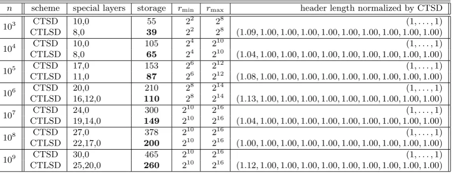
Table 6: Comparison of the storage and the expected header lengths for the CTSD and the CTLSD schemes.
satisfying this condition. Similarly the computation of E[Zn,ri ] is carried out. Overall, the complexity of the algorithm is still O(rlog2n).
There is one complication that we have not explained. This is the problem of characterizing the dividing path and counting the number of nodes at the same level and on the same side of the dividing path. It turns out that given the value ofn, this can always be done. The details are provided in [BSar] and so are omitted here. We have incorporated these in our implementation of the algorithm to compute expected header length given any value of nand r.
The expected header length of the CTLSD method is E[Yn,r]. As given in (12), this quantity is
equal to the sum of E[Xn,r] andE[Zn,r]. We have shown that E[Zn,r] can be computed in O(rlog2n) time. The quantity E[Xn,r] is the expected header length of the CTSD scheme and can be computed inO(rlogn) time [BSar]. So, the overall complexity of the algorithm isO(rlog2n).
Table 6 provides some examples of running the algorithm for computing expected header length for non-full trees using the CTSD and the CTLSD schemes. The chosen values ofrare 10 equispaced values between rmin and rmax for the respective n. The CTLSD method is run by adopting the constrained
minimization layering strategy where all levels including and below`0− blog2rmincare considered to be
in one layer. The expected header length of the CTLSD method is almost similar to the CTSD scheme while the user storage requirement is a little more than half of the CTSD scheme. Hence, with an assumption on the minimum number of users, the CTLSD scheme with the constrained minimization layering strategy would be the more practical choice.
Since the CTLSD scheme subsumes the LSD scheme, this algorithm computes the expected header length for the LSD scheme too. In [HS02], it was mentioned that the expected header length for their layering scheme, i.e; HS layering is around 2r. As we have seen earlier, by suitably placing the special levels, this can be brought down significantly to about the expected header length of the SD scheme. On the other hand, for the HS layering, the expected header length can also be somewhat larger than 2r. For example, for l0 = 28 andr = 2, the expected header length is 2.23r.