GENERATION OF AN ARTIFICIAL TIME HISTORY MATCHING
MULTIPLE-DAMPING FLOOR DESIGN RESPONSE SPECTRA
Svetlana Durnovtseva1, Peter Vasilyev 2
1 Engineer, CKTI-Vibroseism, Saint Petersburg, Russia (sdurnovtseva@cvs.spb.su) 2 Principal, CKTI-Vibroseism, Saint Petersburg, Russia (peter@cvs.spb.su)
ABSTRACT
The method of generating an artificial time history matching multiple-damping response spectra is proposed. The synthesis algorithm based on spectral analysis and multiparametric optimization is adduced. Advantages of the method developed in comparison with other approaches that operate with only one damping response spectrum are discussed through the example of seismic analysis of feed water pipeline.
INTRODUCTION
Modern approaches to the seismic design of nuclear power facilities mean that in addition to intensity that characterizes level of seismic hazard zone of construction design response spectra (RS) should be taken in consideration.
Time histories matching multiple-damping design response spectra are required for nonlinear analytical models, for structures that have a different damping ratio at their parts and for structures with a local damping such as piping protected by viscous dampers and other restraint devices. This requirement is given in USNRC (2007): “The response spectra obtained from such artificial time histories of ground motion should generally envelop the design response spectra for all damping values to be used”.
Most of the existing methods of time histories synthesis operate with only one damping response spectrum. Let us demonstrate an example of such an approach.
Figures 1 – 3 contain the set of design response spectra (red lines) defined for such damping ratios as 0.5, 2, 5, 10 and 20 %, which will be further denoted as the target set. The time histories matching 0.5, 5 and 20 % spectra were generated and response spectra calculated from these time histories are marked with bold blue lines in Figures 1 – 3 respectively. Thin blue lines in these figures correspond to the spectra calculated for the remaining damping ratios.
Figure 2. Blue lines – set of response spectra matching time-history generated for 5 % damping response spectrum, red lines – target set, bold lines – 5 % damping response spectra.
Figure 3. Blue lines – set of response spectra matching time-history generated for 20 % damping response spectrum, red lines – target set, bold lines – 20 % damping response spectra.
SOLUTION TO THE PROBLEM
It is extremely complicated to find a time history matching multiple-damping spectra in time domain because representation of signal in time domain doesn't give any information about frequency components. The Fourier transform which makes it possible to get spectral representation of signal (dependence of amplitude upon frequency) shall be applied to find an artificial time history. The proposed method for the synthesis of time histories is iterative and consists of the following steps:
- choice of the initial approximation;
- forming the optimization parameters' vector; - evaluation of the goal function;
- minimization of the goal function; - finding the solution.
Choice of the Initial A
pproximationGenerated time histories should meet requirements of the regulatory design guides. Some of these requirements impose restrictions on choice of the initial approximation. Thus, according to ASCE/SEI 43-05 (2043-05) records shall have a time increment
dt
of at most 0.01 s. Artificial time histories shall benumerically developed so that they reasonably represent the ground motion expected for the site. Duration enveloping function parameters depending on magnitude are presented in Table 1.
Table 1: Duration enveloping function parameters. Magnitude Rise time, sec (
r
t
) Duration of strongmotion, sec (
t
m)Decay time, sec (
t
d)7,0-7,5 2 13 9
6,5-7,0 1,5 10 7
6,0-6,5 1 7 5
5,5-6,0 1 6 4
5,0-5,5 1 5 4
The research is operated with the enveloping function
f
env of the form
.
,
4
2
sin
;
,
1
;
0
,
4
2
sin
)
(
d m r m r d m r r r r envt
t
t
t
t
t
t
t
t
t
t
t
t
t
t
t
t
f
Knowing a time increment and enveloping function it is possible to define the number of points of desired time history as
np
(
t
r
t
m
t
d)
/
dt
. Since the algorithms of the fast Fourier transform (FFT) run at maximal speed when number of points is equal to a power of two, let us put the number of points of the time history kN
2
so that2
k1
np
2
k. Herewith formally the duration of the timehistory (and hence the duration of the enveloping function) increases on
(
N
np
)
dt
seconds. However, let us assume thatf
env(
t
)
0
witht
r
t
m
t
d
t
t
r
t
m
t
d
(
N
np
)
dt
. This assumption allows to keep the shape of the enveloping function satisfying ASCE 4-98 (1998) and obtain the optimal number of parameters for the FFT.Obviously, the seismic action is by nature superposition of harmonics. Let the number of harmonic components beN/21, then it is possible to form an initial approximation to the solution. Let
us assume amplitudes and phase of harmonics are equal to random numbers in ranges from 0 to 1 and from 0 to
2
respectively. Further it is necessary to assemble the time history as the superposition of declared harmonics, multiply it by the enveloping function and find the maximum absolute value of received time history – maxt a0(t). Finally corrected initial approximation to the solution can be found bymultiplying the amplitudes by value
) (
0
max
a t ZPAt
, where ZPA – zero-period acceleration.
Forming the Optimization Parameters’ Vector
Applying the Fourier transform to the initial approximation, we obtain N ik t k
k
e
X
t
a
1)
(
,where
X
k – k-th complex amplitude,k
– k-th circular frequency of the harmonic oscillation. Theswitch from the coefficients of the Fourier transform to the amplitudes and phases of the harmonics contained in the original signal will yield
. 2 / ,1 , ) Re( ) Im( , )) Im( ) (Re( 1 ________ N k X X arctg X X N A k k k k k k
Then the optimization parameters’ vector isx[A1,A2,...,AN/2,
1,
2,...,
N/2]N1.Evaluation of the Goal Function
At each iteration the value of the goal function is evaluated in the parameter space as the difference between the original spectra and the spectra calculated from the current approximation to the solution: 2 / 1 2 arg 1 )) ( ) ( ( 1 1 )} ( {
jcurrent ett j J
j
j RS RS
nfreq J
t a
f . (1)
Here RSjtarget – j-th original (target) response spectrum,
RS
jcurrent – the current approximation to thej-th target response spectrum, J – number of spectra, j
nfreq – number of frequencies of j-th RS.
to 50 Hz or the Nyquist frequency. The comparison of the response spectrum obtained from the artificial ground motion time history with the target response spectrum shall be made at each frequency computed in the frequency range of interest.
In practice, the original spectra are often defined at a small amount of points. So before the goal function is evaluated, the target response spectra should be interpolated in the new frequency range which is found by the rule
i1
i(1
j), where j – damping of j-th spectrum.For computation of RS the equation of the oscillator
) (
2 x 2x a t
x
(where
x
,
x
and x – acceleration, velocity and displacement correspondingly, – oscillator’s circularfrequency, – damping coefficient) is numerically integrated for the entire range of frequencies and all damping ratios. Function a(t) in the right part of this equation is restored by inverse Fourier transform of parameters’ vector at the current iteration. Additionally the current approximation to the time-history of ground motion is enveloped, i.e. multiplied by the enveloping function, and finally passed as an argument to the goal function.
Obviously, the presence of high frequencies in the Fourier spectrum leads to an unacceptable increase of the RS in the high-frequency region. To avoid it the Fourier coefficients corresponding to high frequencies are considered equal to zero. The procedure for cutting high frequencies is implemented as follows.
There is a well-known Nyquist-Kotelnikov sampling theorem (Marple (1987)), which states: if a function contains no frequencies higher than B hertz, it is completely determined by giving its ordinates at a series of points spaced 1/(2B) seconds apart. The theorem provides a way to calculate the frequencies at which the original signal is decomposed in the Fourier spectrum. If dt – sampling interval, N – number of samples, then the Nyquist frequency is equal to Nyq1/2dt.
Since the FFT algorithm shifts a negative part of the Fourier spectrum to the right, one can construct the Fourier spectrum for N 1 frequencies from Nyq to Nyq in increments 1/Ndt. In this case X0 corresponds to the frequency 0, positive frequencies are in the range of numbers from 1 to N/2, the remaining values correspond to negative frequencies.
If cut-off frequency is set equal to cut, it is possible to find such a number k in the range of
negative frequencies that the following inequality is fairly: k cut k1. Then to avoid an unacceptable
increase of RS at the right of cut it is sufficient to let Xi 0 with iN/2ncut...N/2ncut, where
k N ncut .
Figures 5, 6 show an application of the described method for cut 30Hz.
Figure 5. Procedure for cutting high frequencies. Response spectra calculated from time histories in Figure 6 (blue – before procedure, red – after procedure).
10-1 100 101 102 103 0
5 10
Frequency, Hz
A
cc
el
era
tio
n,
m
/s
ec
Figure 6. Procedure for cutting high frequencies. Time histories and Fourier spectra (blue – before procedure, red – after procedure).
Minimization of the Goal Function
A modified Hooke-Jeeves algorithm (Bunday (1984)) is used for minimizing the goal function. The Hooke and Jeeves method for finding an optimal solution consist of two kinds of moves: an exploratory move and a pattern one. The exploratory move is accomplished by doing a coordinate search in one pass through all the variables. This gives a new "base point" from which a pattern move is made. The pattern move is a jump in the pattern direction determined by subtracting the current base point from the previous base point.
Considering the procedure for cutting high frequencies the number of optimization parameters is reduced to N 2ncut. For instance, if duration of desired time history is 40 seconds, time increment is
0.01 sec and cut-off frequency is defined as 30 Hz, then the number of points np4000, the number of
parameters 2124096
N , the Nyquist frequency
Nyq
50
Hz,n
cut
819
, so in this case thenumber of optimization parameters can be reduced from 4096 to 2458.
Suppose the initial base point is x[A1,A2,...,AN/2ncut,1,2,...,N/2ncut](N2ncut)1 and
increments for the variables of x are
____ __________ __________ __________ ________ __________ 0 2 , 1 2 / , 2 / , 1 , ) ( max 2 cut cut cut t i n N n N i if n N i if t a ZPA step .
In the classical Hooke-Jeeves algorithm if the coordinate search through all variables does not improve the goal function, the exploratory move is repeated in the same base point but increments should be twice reduced. Let us modify the algorithm as follows: the increments should be divided in half if there are only few successful steps during a coordinate search (less than 20 % of total number of parameters) or
05 . 0 1 i i i f f
f . A step is defined as successful if it improves the goal function. The ratio
i i i
f f f 1 0 5 10 15 20 25 30 35 40 45 50
0 0.02 0.04 0.06 0.08 0.1 0.12 0.14 Frequency, Hz A m pl itu de
shows how quickly the goal function decreases, the increments are considered inefficient for further optimization in case of falling this value lower than 0.05.
The clear distinction between the modified algorithm and the classical one is that in the modified algorithm a pattern move is repeated while the goal function improves, whereas in the classical version a pattern move is applied only once after every exploratory move.
Finding the Solution
Desired time history is a minimum point of the goal function:
(
)
.
min
arg
)
(
t
f
a
t
a
There is a great amount of time histories matching target set of RS. In general, the ideal solution of the problem (
f
{
a
(
t
)}
0
) does not exist for reasonable restrictions on the time history duration. So the aimof this research is to find one of the goal function local minimum, but not the global one. If the obtained time history meets the requirements of various regulatory guides, the problem is considered solved.
PRACTICAL APPLICATION OF THE PROPOSED METHOD
Benefits of the proposed method of an artificial time history generation are shown in this section through the example of seismic analysis of a feed water pipeline located between a steam generator and a hermetic penetration. The computer model of the above-mentioned structure was created by means of dPIPE5 (2007) software and is presented in Figure 7.
Figure 7. Pipeline model.
Seismic characteristics at the pipeline elevation level were given by set of three-directional time histories. Model analysis results without dampers in the system where this set was used as an input excitation were considered as standards. Hereafter the three-directional set of response spectra for 2, 5 and 10 % damping was calculated from given time histories and called the target set. Then 10 sets of three-directional artificial time histories matching the target set were generated by the proposed method (hereinafter denoted as Approach A). It should be noted that any number of time histories’ sets is available due to randomness in choice of initial approximation. Another 10 sets adequately matching only 5 % damping RS were generated by methods mentioned in the introduction (hereinafter denoted as
main steam pipeline
viscous dampers
steam generator
reactor coolant pump feed water
pipeline anchors
spring hangers
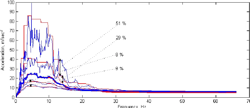
Approach B). An example of data for X-direction syntheses is presented in Figure 8, the mean percentage errors are given in parentheses. The left part of Figure 8 shows the target set of RS (red lines in the top plot) computed from the original time history (red line in the bottom plot), the time history generated by the proposed method (blue line in the bottom plot) and the set of RS calculated from the obtained time history (blue lines in the top plot). The right part of Figure 8 illustrates the time history generated during Approach B (the bottom plot) for 5 % damping RS in the top plot; the compatibility of this time history with the remaining RS in the target set is shown in the middle plot.
Approach A Approach B
Figure 8. X-direction data: original and generated time histories, target and calculated RS.
As to the accuracy of syntheses, the time histories obtained by Approach A are such that each goal function determined in Equation 1 is less than 0.1. Mean percentage errors of all calculated sets of spectra at linearly distributed points in range from 0.05 to 50 Hz with increments of 0.05 Hz are displayed in Tables 2, 3.
Table 2: Mean percentage errors of calculated RS sets. Approach A.
2 % 5 % 10 %
X 0.3177 -0.2047 -0.2829 Y -0.4186 -0.1831 -0.1476 Z 1.3672 1.7129 1.9122
Table 3: Mean percentage errors of calculated RS sets. Approach B.
2 % 5 % 10 %
The output values which were compared with the standards are stresses in the 62 nodes of the feed water pipeline, loads on the 6 spring hangers and on the 7 sliding supports, 6 forces and 6 moments at the anchors, loads on the 10 snubbers, so 97 values for each of 10 sets were considered. The percentage errors of the values observed by both approaches to the standards were computed. The probability density functions of the percentage errors in comparison with the probability density functions of the normal distribution with the same mathematical expectations and dispersions 2 are pictured in Figure 9.
Figure 9. Probability density functions (blue bars – the percentage errors, red lines – normal distribution) in case of the original pipeline’s model.
A similar research was held for the same model equipped with dampers. The obtained results are shown in Figure 10. Apparently, Approach A yields smaller stretching of percentage errors in both analyses. Moreover, a standard deviation of the errors in case of Approach A decreased after adding dampers, but became even larger in case of Approach B. Besides, essential displacement of a mathematical expectation from zero in a positive way in case of Approach B indicates the conservatism of the analysis.
Figure 10. Probability density functions (blue bars – the percentage errors, red lines – normal distribution) in case of the pipeline’s model with dampers.
CONCLUSION
feed water pipeline that used generated time histories demonstrates obvious advantages of the developed method, especially in case of installation of viscous dampers as well as other non-linear restraints.
REFERENCES
ASCE 4-98 (1998). Seismic Analysis of Safety Related Nuclear Structures and Commentary, American Society of Civil Engineers, Reston.
ASCE/SEI 43-05 (2005). Seismic Design Criteria for Structures, Systems, and Components in Nuclear Facilities, American Society of Civil Engineers, Reston.
Bunday, B. D. (1984). Basic Optimisation Methods, Edward Arnold, London. dPIPE 5 (2007). Verification Report, VR01-07, CKTI-Vibroseism.