Sensitivity Analysis of Topology Control for Wireless Adhoc Networks to meet QoS requirements

(1)

Sensitivity Analysis of Topology Control for

Wireless Adhoc Networks to meet QoS

requirements

Ashish Tiwari

1

, O G Kakde

2

Assistant Professor, Department of Computer Science, Visvesvaraya National Institute of Technology, Nagpur, India

Professor, Department of Computer Science, Visvesvaraya National Institute of Technology, Nagpur, India

ABSTRACT:This paper analyzes a technique for topology control (TC) of wireless nodes to meet Quality of Service

(QoS) requirements between source and destination node pairs. Given a set of QoS requirements, a set of wireless nodes and their initial positions, the goal is to find a topology of the nodes by adjusting the transmitting power, which will meet the QoS requirements under the presence of interference and at the same time minimize the energy consumed. The problem of TC is treated like an optimization problem and the technique of Linear Programming (LP) is used to solve it. Sensitivity Analysis is done on the solution obtained after solving the optimization problem. This information is helpful to analyze the behaviour of the optimal topology subject to the variation of QoS constraints and

node characteristics.

KEYWORDS: Wireless Networks; Conflict Graph; Linear Programming; Quality of Service; Topology Control; Sensitivity Analysis.

I. INTRODUCTION

Topology control is the process of coordinating nodes’ decisions regarding their transmitting ranges, in order to generate a network with the desired properties while reducing node energy consumption and/or increasing network capacity [1]. TC is required in adhoc wireless networks because there is no central infrastructure to ensure communications. This means that the nodes themselves have the responsibility of ensuring communication. TC provides an effective way of achieving this goal. By using TC, a network topology of the nodes can be constructed which will have the desired properties (in this case meet the QoS requirements) and reduce the node energy consumption and interference between nodes. The topology of the network can be controlled by controlling which links are allowed to be present or absent in the network. In a wireless network, a link is present between two nodes, if both of them are within range of each other. Thus in this case topology control boils down to controlling the transmitting ranges i.e., the transmitting power of the nodes.

In this paper TC is presented as an optimization problem, where the objective is to minimize the overall energy consumed by all the nodes in the network and the constraints are the QoS requirements and interference.

A QoS requirement is a Service Level Agreement (SLA) between a pair of nodes to maintain certain values of communication parameters like bandwidth, delay, hop count etc., The QoS requirements considered in this paper are the traffic bandwidth and the maximum hop count. Given a set of nodes placed on a two dimensional plane and the QoS requirements between node pairs (source, destination), an optimal topology is found which will meet these requirements in the presence of interference and at the same time reduce energy consumption.

(2)

Copyright to IJIRCCE DOI: 10.15680/IJIRCCE.2015. 0310088 10191

II. RELATED WORK

This paper is mainly an extension of the work of Tiwari et al.,[2] . In [2] an integer linear programming (ILP) formulation of the QoS TC problem is provided for source-destination node pairs and the ILP problem is solved to obtain an optimal topology meeting the QoS requirements. However the issue of interference is not addressed.

In [3], the authors provide a way of multicast routing between multiple hosts on a network which meets the QoS requirements such as end to end delay and bandwidth requirements. They propose a multi-cast tree selection algorithm based on non-dominated sorting technique of genetic algorithm to simultaneously optimize multiple QoS parameters. In [4], the impact of interference on the throughput of wireless networks is studied. Techniques for computing bounds on the throughput of the network in the presence of interference are provided. The concept of a conflict graph to model interference between wireless links is used. Again an LP formulation to optimize the network throughput under the influence of interference is used. In [5], the authors show how interference aware routing can be done to ensure bandwidth provisioning along the path of wireless hops from source to destination.

As far as the authors feel such a detailed sensitivity analysis of ILP formulations for optimal topology has not been carried out.

III.SYSTEM MODEL AND ASSUMPTIONS

A graph G(V,E) represents a wireless network, where each wireless node is a vertex in V and each wireless link

between two nodes is an edge in E. The assumption of bidirectional links is made; hence G is an undirected graph. An

edge e (i, j) exists between nodes i and j if and only if both i and j are within range of each other. The widely adopted

transmitting power model is used, again as in [6], i.e., if di, j is the distance between nodes i and j, then the transmitting

power required to establish a link e (i, j) is,

,

i j i j

P



d

 (1)

Where α is the path loss constant, which typically is taken between 2 and 4.

Thus e (i, j) is in E only if transmitting power Ti , of i, is such that

T

i

d

i j,





and transmitting power of j,

T

_j



d

_{i j}_, .

It is assumed that the nodes are placed on a two dimensional plane with given initial positions (x, y), and that each

node has similar characteristics like maximum node bandwidth capacity (B) and maximum threshold transmitting power

(Pmax). However each node i, may have a different maximum transmitting power Pi , which depends on the battery energy

level Ei , of the node, and the duration D, over which time the traffic has to be maintained. Thus,

/

i i

P



E

D

. (2)

Pi can be between 0 and Pmax. The actual transmitting power of node i, denoted by Ti, can be varied between 0 and Pi

to adjust the transmitting range of i.

The concept of a conflict graph as in [4] is also used in the proposed method to check for interference feasibility.

Each edge in E is a vertex in CG. There exists an edge between two vertices v1 and v2 in CG, if the edges e1 and e2 in E

corresponding to these two vertices in CG, interfere with each other. A graph or topology is interference feasible if it can

maintain the desired properties (in our case meet the QoS requirements) even under the presence of interference

IV. PROBLEM DEFINITION

A set of wireless nodes along with their initial positions (x, y), the maximum node bandwidth B, the maximum

threshold transmitting power Pmax of the nodes, and the maximum transmitting power Pi of each node i (based on the

battery energy level of the node and the duration) are given. A set of QoS requirements is also given in the form of

source, destination (s, d) pairs of nodes. For each pair the maximum hopcount (hs,d) and bandwidth (bs,d) is specified, i.e.,

the traffic of each (s,d) pair should only go over a path whose hop count is less than or equal to the specified maximum

hop count (hs,d) and each node along the path should be able to carry traffic of bandwidth bs,d .

The problem now is to find an optimal topology from the initial topology (which can be obtained from the given

values of (x, y) and Pi) such that the QoS requirements for each pair (s, d) is met, the transmitting power of the nodes is

(3)

V. PROPOSED METHOD

The proposed method involves formulating the problem of TC as an optimization problem and solving it using LP.

Briefly, the initial topology or graph G(V,E) of the wireless network is constructed, an integer linear programming

(ILP) formulation based on this graph is created and solved. The lpsolve C library[7] is used to solve the ILP problem.

The optimal solution obtained will be in the form of the routes to be taken for each (s, d) pair. Depending on this, the

transmitting power of each node (Ti) is adjusted so that the edges required in the route can be formed. This is the actual

TC step. However by adjusting Ti the topology of the graph would have altered. So, a different topology would have

been obtained which is optimal as far as the QoS requirements are concerned. The next step is to construct a conflict graph (CG) for this resulting optimal graph. The CG is used to determine whether the optimal graph is interference feasible or not. If it is interference feasible, then the optimal solution obtained using LP is the final solution.

The underlying sections discuss the method in detail.

A. Constructing the initial network graph

Using the previously discussed condition (1) and the given initial values of Pi and (x, y) of each node i, one can easily

determine which edges are present or absent and hence construct the graph G(V,E) representing the initial topology.

Initially for each node i, set Ti = Pi, and determine which other nodes are in range, this helps determine which edges

are present or absent. For convenience’s sake each edge is labelled with the power required to maintain that edge.

B. ILP formulation

The ILP formulation is very similar to the one in [6], except for minor changes.

Given,

( , )

G V E

- the graph or initial topology of the network;

B

- maximum node bandwidth capacity

,

s d

b

– traffic bandwidth required for each node pair (s,d);

h

_{s d}_, – the maximum allowed hop count for each node pair

(s,d)

Variables,

,

i j

x

– binary variables,

x

i j, = 1, if there is a link between i and j, otherwise

x

i j, = 0.

, ,

s d i j

x

_{– binary variables, this indicates the route taken from s to d.}

x

_{i j}s d_,, _{= 1, if the route from s to d goes through the link}

(i, j). Note that

, ,

s d i j

x

_{is used to indicate the direction of the route, i.e., if}

x

_{i j}s d_,, _{= 1, then the traffic flows from i to j. This}

means that for a particular (s, d) pair,

, ,

s d i j

x

_and ,,

s d j i

x

_{cannot both be 1.}

Objective function,

Minimize



P x

i j i j, ,



( , )

i j



E

(3)

i.e., minimize the transmitting power of the nodes.

Constraints,

Topology constraints (undirected graph),

,

i j

x

=

x

j i, ,



( , )

i j



E

(4)

This constraint is required for an undirected graph.

(4)

Copyright to IJIRCCE DOI: 10.15680/IJIRCCE.2015. 0310088 10193 , , , ( , )

( , )

s d i j s d i j E

x

h

s d

 







(5)

This ensures that the path from s to d does not have a hop count greater than the maximum allowed.

Bandwidth constraint,

For each node

i V



,

, ,

, , , ,

( , ) ( , ) ( , ) ( , )

s d s d

i j s d j i s d

s d i j E s d j i E

x b

B

   





 

(6)

To ensure that the bandwidth capacity of a node is not exceeded, it takes both incoming and outgoing traffic into account.

This completes the ILP formulation. For more details on implementation see [2]. This is solved using the lpsolve

library[7] .

C. Constructing the resulting topology

The result obtained after solving the LP problem will be in the form of values of 1’s and 0’s assigned to each of

, i j

x

and , , s d i j

x

_{. Using this one can easily deduce the path or route to be taken from s to d for each (s, d) pair and hence}

the transmitting power Ti to be set for each node i.

For example if (2, 4) and (6, 1) are two (s, d) pairs mentioned, and after solving LP the routes obtained are 2354 and

6371. Then the transmitting power of node 2, T2 should be set to a value =

d

_2,3



. Similarly T3 should be set to a value,

3

max(

2,3

,

3,5

,

3,6

,

3,7

)

T



d



d



d



d

 , and so on.

Once the transmitting power for all nodes has been set, the resulting topology is obtained, which is optimal with respect to the QoS constraints, but may or may not be interference feasible.

It may not necessarily be that the resulting topology will only have those edges in the route from s to d, additional edges may get added as a consequence of adjusting the transmitting power of the nodes. This is because of the condition

(1), i.e., as in the previously mentioned example, if T2 is set to a value

d

2,3



, then this may result in the edge (2, 1) also

getting added in addition to the edge (2, 3) because the transmitting power of node 1, T1 is set to a value

d

1,7

 _{, which}

may be sufficient to reach node 2 also. An important point to be noted is that, the routes obtained are used to construct the final topology, therefore the traffic should also be actually routed along the same path from source to destination in the final topology, otherwise the topology will no longer be optimal. Any additional edges that get added into the topology as mentioned before must not be used for routing the traffic.

D. Checking interference feasibility

The next step is to check whether the optimal topology is interference feasible or not. For this the conflict graph is

constructed, as mentioned earlier. Let R(V, E) be the optimal topology obtained and CG(V′, E′ ) be the conflict graph.

The basic idea of checking for interference feasibility is that, no two adjacent vertices in CG should be allocated the same timeslots. A simple algorithm is written which does this check. An LP formulation can also be used to do the same. More details can be found in [8].

VI. EXPERIMENTALDESIGN

A. Simulation Setup

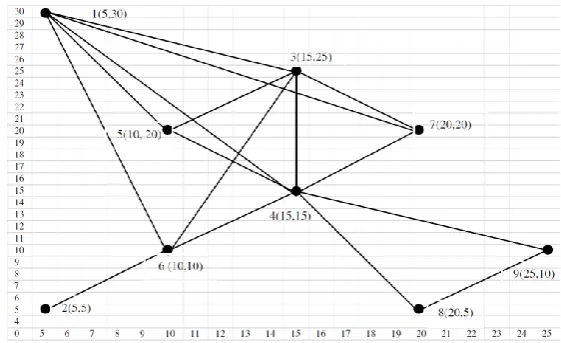
Assume a wireless network with 9 nodes (numbered 1, 2, 3…..9), within a 30x30m square. The initial positions of the nodes are – (5, 30) (5, 5) (15, 25) (15, 15) (10, 20) (10, 10) (20, 20) (20,5) (25,10). The maximum transmitting power

is, Pi = 450 for all nodes i and Pmax = 450. The maximum node bandwidth capacity, is B = 500. The QoS requirements

(5)

B2, 7 = 200, b1, 8 = 150 and b6, 9 = 100; H2, 7 = 4, h1, 8 = 4 and h6, 9 = 4.

The initial topology obtained by setting Ti = Pi = 450 for each node i is shown in Figure 1.

Constructing the ILP formulation for this graph and the given QoS requirements is done according to the equations

(3) – (11). On solving this ILP problem using lpsolve, the values of the variables are obtained. The optimal routes are

found by

, ,

s d i j

x

_{variables which are equal to 1. The optimal routes are summarized in Table 1.}

TABLE 1: Optimal Routes for QoS requests

s d

b

_{s d}_, Optimal Route

2 7 200 2637

1 8 150 15498

6 9 100 61549

Based on this the transmitting power to be set for each node is, T1 = 425, T2 = 50, T3 = 250, T4 = 125, T5 = 125, T6 =

425, T7 = 50, T8 = 50, and T9 = 125. The resulting topology (using condition (1)) is shown in Figure 2.

Figure 1. Initial topology

(6)

B. Simulation Results and Sensitivity Analysis

The simulations were run to optimize the total transmitting power of nodes satisfying various QoS requirements. The optimal topology generated was evaluated in terms of the total transmitting power (P) and also the time taken to

achieve the optimal topology (T_opt).

1) Impact of hop count on Topology

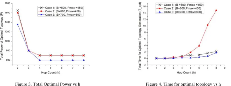
The objective was to evaluate the sensitivity of the topology as a function of the hop count QoS requirement. The results are plotted in Figure 3 and Figure 4 for P vs h and T_opt vs h respectively. There were 3 cases considered, namely

a) Case 1: The node bandwidth for all nodes is B=500 and maximum transmitting power for all nodes is

Pmax=450.

The bandwidth was chosen such that the average bandwidth demand per request is 0.3B, whereas the Pmax was

chosen such that the initial graph remains connected. This can be thought of as a minimum case for evaluation. Then with these parameters fixed, the hop count was varied from 1 to 8. As is evident from the graph the optimal power decreases as the hop count constraint is relaxed and stabilizes at a value of 700 for hop count value of 4. There is no further improvement in the solution on further relaxation althought the time to compute the optimal solution increases. For the case of hop count=1, there is "no solution" and the time to decide that is 0.012s which is the fastest for this case.

b) Case 2: The node bandwidth for all nodes is B=600 and maximum transmitting power for all nodes is

Pmax=450.

chosen such that the initial graph remains connected. This can be thought of as an average case for evaluation. As is evident from the graph the optimal power decreases as the hop count constraint is relaxed and stabilizes at a value of 700 for hop count value of 4.

c) Case 3: The node bandwidth for all nodes is B=700 and maximum transmitting power for all nodes is

Pmax=800.

chosen such that the initial graph remains almost fully connected. This can be thought of as a maximum case for evaluation. As is evident from the graph the optimal power decreases as the hop count constraint is relaxed and stabilizes at a value of 600 for hop count value of 4.

2) Impact of node bandwidth on Topology

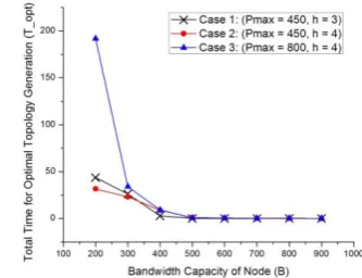
The objective was to evaluate the sensitivity of the topology as a function of the bandwidth capacity of a node B. The results are plotted in Figure 5 and Figure 6 for P vs B and T_opt vs B respectively. There were 3 cases considered, namely

a) Case 1: The maximum tranmitting power of each node is Pmax=450 and hop count is h=3.

The hop count and maximum transmitting power of each node was chosen such that the initial graph remains connected and an optimal solution is feasible. This can be thought of as a minimum case for evaluation. As is evident from the graph, the optimal power decreases as the bandwidth capacity of a node is increased and stabilizes at a value of

(7)

800 for a B value of 500. There is no further improvement in the solution on further increase of B and moreover the time to compute the optimal solution also decreases. This is due to the fact that more bandwidth at a node can accommodate more traffic paths through it resulting in better and shorter paths. When B is very low, the optimal topology power is peaking at 1850 for B=300, and moreover the solution also converges slowly. This is due to different traffic taking different paths due to low bandwidth capacity of nodes, thereby resulting in more optimal power and more search time. For the case of B=200, there is "no solution" and the time to decide that is 43.593s which is the slowest for this case.

b) Case 2: The maximum tranmitting power of each node is Pmax=450 and hop count is h=4.

The hop count and maximum transmitting power of each node was chosen such that the initial graph remains connected and better optimal solutions are feasible. This can be thought of as an average case for evaluation. As is evident from the graph, the optimal power decreases as the bandwidth capacity of a node is increased and reaches a value of 600 for a B value of 900.

c) Case 3: The maximum tranmitting power of each node is Pmax=800 and hop count is h=4.

The hop count and maximum transmitting power of each node was chosen such that the initial graph is almost fully connected and an optimal solution is feasible. This can be thought of as a maximum case for evaluation. As is evident from the graph, the optimal power decreases as the bandwidth capacity of a node is increased and stabilizes at a value of 600 for a B value of 700.

3) Impact of maximum transmitting power on Topology

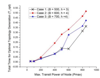
The objective was to evaluate the sensitivity of the topology as functions of the maximum transmit power of each

node. The results are plotted in Figure 7 and Figure 8 for P vs Pmax and T_opt vs Pmax respectively. There were 3 cases

considered, namely

a) Case 1: The node bandwidth for all nodes is B=500 and hop count is h=3.

The bandwidth was chosen such that the average bandwidth demand per request is 0.3B, whereas the hop count hopes for the existence of an optimal solution. This can be thought of as a minimum case for evaluation. As is evident

from the graph the optimal power decreases as Pmax is increased and stabilizes at a value of 800 for Pmax value of 400.

There is no further improvement in the solution on further relaxation and moreover the time to compute the optimal solution also increases marginally. This is due to the fact that a higher maximum transmit power makes the graph more

connected however at the same time increases the number of long edges. When Pmax is very low due to less edges , the

optimal topology power is peaking at 1100 for Pmax=200, however the solution converges fast.

b) Case 2: The node bandwidth for all nodes is B=600 and hop count is h=3.

The bandwidth was chosen such that the average bandwidth demand per request is 0.25B, whereas the hop count hopes for the existence of an optimal solution. This can be thought of as an average case for evaluation. As is evident

from the graph the optimal power decreases as Pmax is increased and stabilizes at a value of 700 for Pmax value of 400.

(8)

c) Case 3: The node bandwidth for all nodes is B=700 and hop count is h=4.

The bandwidth was chosen such that the average bandwidth demand per request is 0.2B, whereas the hop count hopes for the existence of better optimal solutions. This can be thought of as a maximum case for evaluation. As is

evident from the graph the optimal power decreases as Pmax is increased and stabilizes at a value of 600 for Pmax value of

800.

VII. CONCLUSIONS AND FUTURE WORK

We have discussed the formulation of the energy efficient QoS topology control problem. The adhoc network is characterized by a lot of assumptions on the traffic pattern, node characteristics and QoS requirements which makes the optimal solution less intuitive. Sensitivity analysis on the optimal topology can make us assess the impact of various parameters on the solution obtained. This way we can gain an insight as to which parameters affect the optimal solution in which way. This is the first time in the literature that sensitivity analysis of topology control is studied regarding to QoS provisions and node characteristics. Each case of QoS parameters and node maximum transmitting powers has been considered. For the former case, we considered both bandwidth and delay bound as QoS requirements. The problem has been formulated as an integer linear programming problem. Extensive simulations were done to assess the variation of total power of the optimal topology and also time to obtain the optimal topology. By configuring a good QoS topology and judiciously choosing node parameters, QoS requests can be best served in the system. The price paid to achieve a desired adhoc network in terms of energy and time can be proposed to balance the two.

So far a technique for sensitivity analysis of TC has been provided. But further study of this technique is required. In particular, investigate the possibility to rank parameters in order of influence. Formally analyze the relation between the cost function and the samples. Try to find out methods that reduce the computational effort to do sensitivity analysis.

REFERENCES

1. G. Paolo Santi, “Topology Control”, in Topology Control in Wireless Ad Hoc and Sensor Networks, John Wiley & Sons Ltd, 2005, pp 27-34.

2. Yadu, Kishore K., Ashish Tiwari, and O. G. Kakde. "Optimization based topology control for wireless ad hoc networks to meet QoS requirements."

In Reliable Distributed Systems, 2010 29th IEEE Symposium on, pp. 30-36. IEEE, 2010.

3. Abhishek Roy, Nilanjan Banerjee, Sajal K. Das, “An efficient multi objective QoS-routing algorithm for wireless multicasting”, Vehicular

Technology Conference, VTC Spring 2002, IEEE 55th, vol. 3, pp. 1160-1164, August 2002.

4. Kamal Jain, Jitendra Padhye, Venkata N. Padmanabhan, Lili Qiu, “Impact Of Interference On Multi-hop Wireless Network Performance”, Wireless

Networks, Selected papers from ACM MobiCom 2003, vol. 11, issue 4, pp. 471-487, July 2005.

5. Jian Tang, Guoliang Xue and Christopher Chandler, “Interference-aware routing and bandwidth allocation for QoS provisioning in multihop

wireless networks”, Wireless Communications & Mobile Computing, RRM for Next-Generation Wireless and Mobile Communication Systems, vol. 5 , issue 8, pp. 933-943, ACM Dec. 2005.

6. Xiaohua Jia, Deying Li, Dingzhu Du, “QoS Topology Control in Wireless Ad Hoc Networks”, Resource allocation and QoS in Ad Hoc Networks,

Proceedings IEEE INFOCOM 2004, March 2004.

7. Michel Berkelaar et al., the lpSolve project, ver. 5.5.0.15, Available: http://sourceforge.net/projects/lpsolve/, Feb. 2012.

8. Anuj Mehrotra and Michael A. Trick, “A column generation approach for graph coloring”, Informs Journal on Computing, vol. 8, No. 4, pp.

344-354, Fall 1996.