HIGHLIGHTED ARTICLE
| GENOMIC SELECTION
A Simple Test Identi
fi
es Selection on Complex Traits
Tim Beissinger,*,†,‡,1Jochen Kruppa,§,** David Cavero,††Ngoc-Thuy Ha,§Malena Erbe,‡‡ and Henner Simianer§,1
* Plant Genetics Research Unit, U. S. Department of Agriculture–Agricultural Research Service, Columbia, Missouri 65211,†Division of Biological Sciences, and‡Division of Plant Sciences, University of Missouri, Columbia, Missouri 65211,§Center for Integrated Breeding Research, University of Göttingen, 37075, Germany, **Institute for Animal Breeding and Genetics, University of Veterinary Medicine Hannover, 30559, Germany,††H&N International, 27472 Cuxhaven, Germany, and‡‡Institute for Animal Breeding, Bavarian State Research Centre for Agriculture, 85586 Grub, Germany
ABSTRACTImportant traits in agricultural, natural, and human populations are increasingly being shown to be under the control of many genes that individually contribute only a small proportion of genetic variation. However, the majority of modern tools in quantitative and population genetics, including genome-wide association studies and selection-mapping protocols, are designed to identify individual genes with large effects. We have developed an approach to identify traits that have been under selection and are controlled by large numbers of loci. In contrast to existing methods, our technique uses additive-effects estimates from all available markers, and relates these estimates to allele-frequency change over time. Using this information, we generate a composite statistic, denotedG^;which can be used to test for significant evidence of selection on a trait. Our test requires pre- and postselection genotypic data but only a single time point with phenotypic information. Simulations demonstrate thatG^ is powerful for identifying selection, particularly in situations where the trait being tested is controlled by many genes, which is precisely the scenario where classical approaches for selection mapping are least powerful. We apply this test to breeding populations of maize and chickens, where we demonstrate the successful identification of selection on traits that are documented to have been under selection.
KEYWORDSchickens; complex traits; maize; selection; GenPred; Shared Data Resources; Genomic Selection
Q
UANTITATIVE traits encompass an inexhaustible num-ber of phenotypes that vary in populations, from char-acters such as height (Yanget al.2010), to weight (Barshet al. 2000), to disease resistance (Polandet al.2009). These types of traits are so essential for agriculture and human health that the entirefield of quantitative genetics revolves around their study (Plominet al.2009; Wallaceet al.2014). However, the nature of quantitative traits makes it difficult to study their genetic basis; for nearly a century, scientists have modeled quantitative traits by assuming that their underlying control involves many loci each contributing a very small proportion togenetic variance (Fisher 1918), the so-called “infinitesimal model.”Therefore, conducting studies with enough power to identify a substantial proportion of the loci that contribute to a quantitative trait requires a massive sample size, impos-ingfinancial and logistical barriers. However, this model of quantitative trait variation does an excellent job when pre-dicting important characteristics such as response to selec-tion (Visscheret al.2008). For instance, genomic prediction methodologies (Meuwissenet al.2001) allow the breeding value and/or phenotype of individuals to be predicted with remarkable precision from genomic information alone.
The models of quantitative genetics have had a less dramatic impact on studies of evolutionary adaptation, where genomes are often scanned to identify adaptive loci with large effects (Akey 2009). Positive selection on such loci leaves behind pronounced signatures, deemed“ selec-tive sweeps.”There is an abundance of evidence for such sweeps in humans (Sabetiet al.2007), natural populations (Schweizeret al. 2016), livestock (Qanbari and Simianer 2014), and crops (Huffordet al.2012). However, alterna-tive forms of selection, including purifying selection against
Copyright © 2018 Beissingeret al.
doi:https://doi.org/10.1534/genetics.118.300857
Manuscript received December 21, 2017; accepted for publication March 10, 2018; published Early Online March 14, 2018.
This is a work of the U.S. Government and is not subject to copyright protection in the United States. Foreign copyrights may apply.
Supplemental material available at Figshare:https://doi.org/10.6084/m9.figshare. 5899267.
new mutations (Lawrie et al. 2013), selection on standing variation (Garud et al. 2015), or selection on many loci of small effect (Turchinet al.2012) rarely leave these dis-cernible signatures at individual loci. Evidence of these forms of selection can be difficult to identify. When they are found, it is often through the pooling of weak evidence at individual loci into a stronger signal across a class of loci. For example, Beissingeret al.(2016) demonstrated the im-portance of purifying selection during maize evolution by combining evidence from all maize genes. An approach implemented by Berg and Coop (2014) tests for evidence of selection on a quantitative trait by evaluating allele fre-quencies at all loci that have previously been implicated by genome-wide association studies (GWAS) as putatively as-sociated with that trait. This approach has since been used to test for selection on multiple human traits, including height (Mathiesonet al. 2015) and telomere length (Hansenet al. 2016).
In studies of model organisms or agricultural species, large collections of previously identified“GWAS hits” are not as abundant as in humans, on which the Berg and Coop (2014) method depends. This is partly due to the more mod-est sample sizes that tend to be used in experimental settings compared to clinical studies, which are often combined in large-scale meta-analyses (Evangelou and Ioannidis 2013). Conversely, genotypic data across at least two time points are often readily available for model and agricultural species. Due to improving technologies for sequencing ancient DNA (Berget al.2017; Mathiesonet al.2018), and/or by leverag-ing populations that have benefited from excellent historical record keeping (Konget al.2017), genetic data with a tem-poral component is increasingly available in humans. We have developed a test for selection on complex traits that leverages such genotype-over-time data. Our test depends on the relationship between the change in allele frequency between two generations and the estimated additive effect of the same allele, computed for every genotyped locus. We use these values to compute an estimate of the direction of genetic gain, which can be shown to be additive across all loci considered. Our estimate lends itself to a simple permuta-tion-based test for significance that avoids many of the de-mographic history- and population structure-related caveats that complicate determining significance when testing for selection (de Villemereuil et al. 2014). The method uses additive-effects estimates for each locus calculated simul-taneously by using shrinkage-based methods that have been honed over the past 15 years for the purpose of ge-nomic selection and prediction (de Los Camposet al.2013). Therefore, this test can be considered analogous to reverse genomic selection; rather than using predictions of breeding value to drive selection and hence future changes in allele frequency, we use the same data coupled with knowledge of past changes in allele frequency to make inferences regarding which traits were effectively under selection in the past. In-terestingly, wefind by simulation that this approach is most powerful for identifying selection on traits controlled by
many loci of small effect, which is exactly the situation where other tests for selection and/or association are least powerful.
Herein, wefirst motivate and describe our test for selection on complex traits, which we callG:b We then perform simula-tions demonstrating the validity of the method and explore the situations where it is most and least powerful. Finally, we apply the method to breeding populations of maize and chicken. In both of these experimental situations, we success-fully identify the traits that are known to have been selected. Collectively, our results demonstrate that this approach may be leveraged to identify novel traits or component traits that may be used to inform future breeding decisions and/or for enhanced historical, ecological, and basic scientific under-standing. Software for implementing this test is provided in the accompanying Github repository:http://github.com/ timbeissinger/ComplexSelection.
Materials and Methods
Theoretical motivation
Assume that a trait is fully controlled by additive di-allelic loci
j¼1;. . .m:The genotypic value,aj, of an allele at locusj, is
then equal to its gene substitution effect,aj. Based on this equivalency, the mean phenotypic effect (Mj) attributable to the locus is given by Mj=aj(2pj21), wherepjis the fre-quency of the reference allele at this locus. It follows that the change in the population mean resulting from selection on this locus, what we may consider the locus-specific response to selection, is given by
Rj¼Mj12Mj0¼ajð2pj121Þ2ajð2pj021Þ ¼2ajðpj12pj0Þ;
wherepj0is the allele frequency before selection andpj1is the allele frequency after selection. DefineDj=(pj12pj0), leading to Rj= 2Djaj. Based on our earlier assumption of complete additiv-ity, summing over allmloci provides a genome-wide estimate of the response to selection (Falconer and Mackay 1996):
b
R¼2X
m
j¼1
Djaj: (1)
Strictly speaking, since relative effect sizes may change each generation with changing allele frequencies throughout the genome, (1) is applicable for a single generation. However, under the assumption of many loci affecting a trait, (1) may approximately apply for many generations of selection. This estimate of selection response also naturally arises from the logic of random regression best linear unbiased prediction (RRBLUP) (Meuwissenet al.2001). Here, a model is used:
y¼XbþZsþe; (2)
whereyis a vector of lengthncontaining phenotypes for a specific trait,barefixed effects,sNð0;Is2
of length m containing additive SNP effects at m loci; eNð0;Is2
eÞis the vector of random residual terms ands2s ands2
e are the corresponding variance components.XandZ are incidence matrices linking observations inyto the respec-tive levels offixed effects inband random SNP effects ins:In more detail,Zis ann3mmatrix where elementzijcontains the genotype of individualiat SNP locusj:Since such models are invariant with respect to linear transformations of the allele coding (Strandén and Christensen 2011), we may use the notation zij¼0;1=2; or 1;standing for zero, one, or two copies of the reference allele. Note that with this coding, sj is equivalent to 2aj in the coding above since it reflects the contrast between the two homozygous genotypes at locusj:Due to the equivalence of genomic BLUP (GBLUP) (VanRaden 2008) and RRBLUP (Endelman 2011), it is pos-sible to calculate genomic breeding values of the genotyped individual asub¼Zbs;where bsare the solutions for the SNP effects obtained using RRBLUP with model (2).
Now assume that individuals in the vector y can be assigned to gdiscrete generations and that the individuals of the oldest generation comefirst and the individuals of the last generation come last. We then can define ag3nmatrix
L¼ 2
4l⋮ ⋱ ⋮1 ⋯ 0 0 ⋯ lg
3 5;
wherelpis a row vector of lengthnp;which is the number of individuals in generationp, of which all elements are 1=np: With this, a vector u of lengthgreflecting average breed-ing values per generation can be calculated asu¼Lbu;and estimated selection response results as Rb¼ug2u1 : Now,
u¼Lbu¼LZbs;whereLZis ag3mmatrix in which element p;j reflects the average allele frequency of the reference al-lele at SNP jin generation p:The allele-frequency change between generation 1 and generationgcan be obtained as a linear contrast between the first and the last row of this matrix as D ¼k9LZ; wherek is a vector of length g with k1¼ 21; kg¼1;and all other elements are 0. Finally, the selection response can be written asbR¼Dbs;which is identi-cal to Equation 1, given thatsis equivalent to 2a:
Furthermore, theory suggests that under the assumption that selection intensity is equal for all loci across the genome, the change of allele frequency Dj should be approximately proportional to the allele effectajsuch that, for a trait under selection, a nonzero correlation between allele-frequency change and the additive effect of alleles on that trait is expected (Wright 1937). Alternatively stated, (1) empha-sizes the temporal component of the Breeder’s equation, R = h2S, whereh2is the narrow-sense heritability of a trait andSis the selection differential. Given a population of individ-uals with two time points of genotypic data, it is simple to compute Dj for every genotyped locus. Furthermore, the shrinkage methods of genomic prediction (de Los Campos et al.2013), including ridge regression (Endelman 2011) and GBLUP (VanRaden 2008), allow additive effects (aj) to be approximated for every genotyped position. For this, a
set of individuals genotyped and phenotyped in at least one generation is needed.
A notable benefit of the estimator in (1) is that by leveraging pre- and postselection data from genotypes rather than from phenotypes, it only requires one genera-tion of phenotyping. Addigenera-tionally, this suggests that if we considerRa random variable, then given the distribution ofR in a scenario without selection, a test of whether or notbRis different from zero may be performed. SinceR^is the genomic response to selection, this is equivalent to testing whether or not a trait has been under selection during the time frame under study.
Test statistic and significance testing
We implemented a permutation-based strategy to test whether or notR^ is significantly different from zero. Genetic drift and selection jointly determine changes in allele frequency,Dj;but without selection these changes in frequency should not be re-lated to effect size or direction. The reverse is also true; effect sizes,aj;are estimated based on a genomic prediction model applied to phenotypes measured in a single panel of individuals. Therefore they are not correlated with changes in allele fre-quency. While a correlation between minor allele frequency (MAF) and the magnitude of SNP effects is possible due to estimation error during genomic prediction; without ongoing selection, allele frequency should not correlate with the direc-tion of SNP effects. This suggests that a null distribudirec-tion forR^in a no-selection scenario may be generated via a permutation approach. Assuming no linkage disequilibrium (LD) between markers, a simple shuffling ofDj andajcan be implemented to generate the desired null distribution. However, LD between markers compromises the applicability of this simplified tech-nique for most populations: such an approach overestimates the sample size of the permutation test by treating each marker as an independent observation, while in reality any level of LD between markers leads to fewer independent observations than markers. Therefore, we have employed a semiparametric method that scales the variance of the permutation test statistic according to the realized extent of LD to alleviate this discrepancy.
null distribution forG^which assumes no selection and com-plete linkage equilibrium.
The central limit theorem dictates that realizations ofbGperm are normally distributed with approximate meanGpermb and SD SEðbGpermÞ: Therefore,s, the underlying SE of a single-locus estimate forGperm;^ is given bys¼SEðGperm^ Þpffiffiffiffim;where SEðGpermb Þis the observed SE ofGperm:b Consider the quantity mind, representing the effective number of independent loci. If the SD of Gpermb was calculated using mind independent markers, its expectation would beSEindðGpermb Þ ¼ s=pffiffiffiffiffiffiffiffiffimind: Plugging in the estimate for sobtained above,SEindðGperm^ Þ becomesSEindðGperm^ Þ ¼ SEðGperm^ Þpffiffiffiffiffiffiffiffiffiffiffiffiffiffiffiffim=mind:
In practice, the above implies that to test for selection, b
G¼Pmj¼1Djajmay be calculated from data, and then a per-muted null distribution for G^ that assumes linkage equilib-rium can be generated. This permutation distribution may then be approximated with a normal distribution, whose var-iance can be scaled according to the effective number of in-dependent markers,mind;which can be efficiently estimated based on LD decay. Ultimately, significance may be evaluated by comparingG^to a normal distribution with meanGpermb and SDSEðGpermb Þpffiffiffiffiffiffiffiffiffiffiffiffiffiffiffiffim=mind:
Simulations
We conducted a series of simulations to evaluate the power of thebGstatistic for identifying selection on complex traits. Ge-notypic data were simulated with the software program QMSim (Sargolzaei and Schenkel 2009). An overview of our simulation strategy at the most general level is that we simulated selection in a generic species with 1000 QTL dispersed along 10 100-cM chromosomes, with a total of 100,000 equally spaced markers (10,000 per chromosome). In thefirst step of each simulation, the total population was established based on 10,000 individuals randomly mating for 5000 generations. Selection then began and simulations pro-ceeded for 20 generations with more control over each gen-eration. Truncation selection was performed based on high phenotype. Except where otherwise noted, 1000 individuals (500 males and 500 females) were permitted to mate each generation out of a population of 5000, providing a selection proportion of 0.2. For each simulation, heritability was set to 0.5. Drift simulations were identical to selection simulations in terms of genome layout and genetic basis of the trait, but individuals were selected randomly.
This general scheme encapsulates characteristics of most plant and animal breeding populations, including the large number of progeny typical of plants and the truncation selec-tion protocol often associated with animal breeding and/or selection in the wild. Additional details regarding the simu-lated population are included in Supplemental Material, Table S1. All simulation scripts can be found at http:// github.com/timbeissinger/ComplexSelection. We varied the specific simulation parameters shown below:
Number of QTL: Genetic architectures with 10, 50, 100, 1000, or 10,000 QTL were simulated.
Number of individuals phenotyped: After selection was sim-ulated, the phenotypes from a subset including 1000, 500, 250, 100, or 50 individuals were sampled and used for estimating SNP effects.
Selected proportion: The respective number of males and females reproducing each generation was always simu-lated to be 500. To vary the selected proportion, we sim-ulated litter sizes of 4, 20, 40, and 200.
Number of generations of selection: Selection simulations were conducted for 1, 10, 20, 50, and 100 generations. Phenotyping generation: For 20-generation simulations,
phe-notypes were analyzed from preselection individuals (gen-eration 0), midselection individuals (gen(gen-eration 10), and postselection individuals (generation 20).
Number of generations after selection: After 20 generations of selection, we evaluated whetherG^was still significant after 5, 20, 50, or 100 generations without selection.
Selection mapping in simulations
For the set of simulations where the number of QTL were varied, pre- and postselection simulated allele frequencies were output from QMSim. These were used to calculate marker-specificFSTvalues, as was performed by Lorenzet al.(2015). FST was computed according toFST¼ s2=½pð12pÞ þs2=2; wheres2is the sample variance of allele frequency between pre- and postselection populations and p is the mean allele frequency (Weir and Cockerham 1984). Experiment-wide 5% significance thresholds were identified based on the 95% FSTquantile observed from drift simulations. These thresholds were applied toFSTvalues obtained from selection simulations to determine detection and false-positive rates. Simulated QTL were declared detected if a significant marker was identified within a 0.1-cM window surrounding the QTL. False positives were defined as markers that were not within a 0.1-cM win-dow surrounding any simulated QTL.
Maize data
All maize data were previously published and described by Lorenzet al.(2015). In brief, a selection index comprising silage-quality traits was used to perform reciprocal recurrent selection. Traits comprising the index were yield, dry matter (DM) content, neutral detergent fiber (NDF), protein con-tent, starch concon-tent, andin vitro digestibility (http://www. cornbreeding.wisc.edu). Phenotypic data includedfive cycles of selection, encompassing20 generations in total. Tens to hundreds of individuals were sampled from each cycle of selection to be genotyped. Genotyping was performed with the MaizeSNP50 BeadChip, which includes 56,110 markers in total (Ganal et al. 2011). After removing monomorphic SNPs, redundant SNPs, quality filtering, and imputing as described in Lorenz et al.(2015), 10,023 informative SNPs remained.
cycle 2 (n= 163) to cycle 5 (n= 211) was computed for each SNP. Since all SNPs were di-allelic, the frequency of only one allele was tracked and the frequency change for that allele perfectly mirrored the change for the other allele. For the tracked allele only, allelic effects were estimated using the R package RR-BLUP (Endelman 2011). Phenotypic informa-tion was available from individuals representing selecinforma-tion cycles 1 through 4 and, since population size was small, we used all phenotyped individuals to estimate SNP effects. To accomplish this without biasing effect estimates due to drift, afixed effect for cycle was included in our model. Our exact analysis scripts are available athttp://github.com/timbeissinger/ ComplexSelection.
Chicken data
Data were available for one white-layer (WL) and one brown-layer (BL) line from a commercial breeding program. Both closed lines have been selected over decades with a similar composite breeding goal which consists of, among others, laying rate, body weight and feed efficiency of the hens, as well as egg weight and egg quality; where the respective weights of the different traits varied between lines and over time. In total, 673 (743) WL (BL) individuals were genotyped, of which.80% were from the last generation and the remain-ing animals were parents, grandparents, and great-grandparents of the actual birds. Complete pedigree data were available for all genotyped individuals and consisted of 2109 (1879) individuals going back 13 (9) generations in WL (BL). The oldest generation was defined as the base population and it comprised 111 (64) ungenotyped individuals and was sep-arated from the majority of genotyped individuals by 12 (8) generations.
Current individuals were genotyped with the Affymetrix Axiom Chicken Genotyping Array which initially carries 580K SNPs. These data were pruned by discarding sex chromo-somes, unmapped linkage groups, and SNPs with MAF,0.5% or genotyping call rate ,97%. Individuals with call rates
,95% were also discarded. Subsequently, missing genotypes at the remaining loci were imputed with Beagle version 3.3.2 (Browning and Browning 2009), resulting in sets of 277,522 (334,143) SNPs for the WL (BL) individuals.
To calculate the allele-frequency change in the chicken populations, the allele frequency in the base population in-dividuals had to be reconstructed by statistical means. This was done using the approach of Gengleret al.(2007), which, in short, considers the allele frequency in an individual as a quantitative and heritable trait and uses a mixed-model ap-proach to obtain a BLUP for the allele frequency of all ungen-otyped individuals. This is done by linking the genungen-otyped offspring to the ungenotyped ancestors via the pedigree in-formation (for details, see Gengleret al.2007). This required solving 277,522 (334,143) linear equation systems of dimen-sion 2109 (1879) for the WL (BL) data set. Next,Difor locusi was calculated as the difference of the observed allele fre-quency of the genotyped individuals in the current and the three ancestral generations and the average estimated allele
frequency of the 111 (64) base population individuals 12 (8) generations back.
For each genotyped individual, conventional (nongenomic) BLUP breeding values and the respective reliabilities for a wide set of traits were available. SNP effects were estimated in a two-step procedure: first, for each trait in each line, genomic breeding values were estimated via GBLUP, fol-lowed by a back-solution of estimated SNP effects. In the GBLUP step, the modely¼1mþZgþewas solved, wherey is the vector of deregressed proofs (DRPs) of genotyped in-dividuals for a specific trait,mis the overall mean, gis the vector of additive genetic values (i.e., genomic breeding val-ues) for all genotyped chickens, eis the vector of residual terms, 1 is a vector of ones, and Zis a squared design ma-trix assigning DRPs to additive genetic values with di-mension number of all genotyped individuals. Residual terms were assumed to be distributed e Nð0; Rs2
eÞ; where R is a diagonal matrix with diagonal elements Rii¼ ½cþ ð12r2
DRPiÞ=r2DRPih2=ð12h2Þ(Garricket al.2009) for an individualiin the training set.r2
DRPiis the reliability of DRP for individualiands2
eis the residual variance usingc set to 0.1. The distribution of additive genetic values is as-sumed to beg Nð0; Gs2
gÞ;wheres 2
g is the additive ge-netic variance andGis a realized genomic relationship matrix which was constructed according to method 1 in VanRaden (2008). Estimation of variance components and genomic breeding values was done with ASReml 3.0 (Gilmouret al. 2009).
Next, estimated SNP effects ^swere obtained following Strandén and Garrick (2009) as
bs¼ 1 2Pm1¼1pið12piÞ
MTG21bg;
whereMis a matrix of dimension number of genotyped individuals 3 number of genotyped SNPs with entry mij¼xij22pj.xij is the genotype of individual iat locusj (coded as 0, 1, or 2, which are counts of the reference allele) andpjis the population frequency of the reference allele at SNPj:
Computational resources
Computation was performed using the University of Missouri Informatics Core Research Facility BioCluster (https://bioinfo. ircf.missouri.edu/). Computational nodes where simulations were performed had 64 cores and 512 GB of RAM. Analysis of maize and chicken data were performed on a mediocre laptop with 8 GB of RAM.
Data availability
Results
Simulations
Simulations identified a wide assortment of scenarios for whichG^ is powerful for identifying traits that have been un-der selection, as well as several potential limitations of the method. Our generalized simulation scenario involved 20 generations of truncation selection in a population of 1000 individuals, with a genetic architecture of 1000 QTL controlling the trait and a heritability of 0.5. Phenotyping was performed on 1000 individuals from thefinal generation of selection. Below, we describe howG^is affected when spe-cific parameters deviate from this scenario.
Number of QTL:We simulated variable numbers of additive QTL-controlling traits, from 10, representing a simple trait controlled by large-effect QTL; to 10,000, representing a highly quantitative trait controlled nearly infinitesimally. QTL were evenly spaced along each chromosome and QTL
themselves were not included in the marker set for analysis. A total of 100 simulations were performed for each level of trait complexity. First, we used these simulations to establish the appropriate number of independent markers,mindas described previously, for this test. We calculated how distant two markers must be to have an expected LD level of R2#0:03:We then counted the total number of blocks of this size genome wide. The 0.03 level was established by performing a grid search of potential values and tuning the false-positive rate (Figure S1). An LD cutoff that is too high leads to a high false-positive rate, while one that is too low weakens the power of the test. For populations similar to those discussed here, we observe that requiringR2#0:03 is appropriate.
When we tested for selection in our simulated data, we observed a direct relationship between the number of QTL controlling a trait and the power ofG^to identify selection on that trait. G^ powerfully identifies selection on highly poly-genic traits, but is not powerful for identifying selection on traits controlled by a small number of QTL. Analyses of the
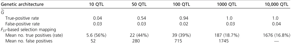
same simulations usingFST-based selection mapping, which involves mapping loci that have been previously subjected to selection (Wisser et al. 2008; Lorenz 2015), showed that traits controlled by a small number of QTL can be mapped using traditional selection-mapping approaches. However, as traits become increasingly polygenic, our simulations dem-onstrate that the ability to map individual, selected genes diminishes (Figure 1). These findings demonstrate how bG and traditional selection mapping can be complementary, depending on the underlying genetic architecture of a trait. Table 1 depicts detection and false-positive rates forGband FST-based mapping under different genetic architectures.
Number of generations:Simulations showed an interesting relationship between the number of generations of selection and the power ofG:^ We observed a definite sweet spot from
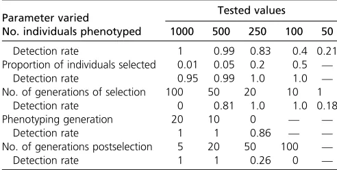
10 to just under 50 generations for whichG^was most pow-erful. Conversely, if selection took place for 100 generations or only for a single generation,G^ became dramatically less powerful (Table 2). We suspect that two forces interact to reduce the power ofG^in the case of a large number of gener-ations of selection. First, over the course of many genergener-ations, our simulated populations became highly inbred, which nota-bly increased LD and therefore reduced mind. Since G^ is summed over markers and then scaled bymind, this substan-tially reduces power. Second, our simulations involved a pre-determined number of QTL withfixed effects at the onset of selection but, as selection persisted, these QTL could be lost to fixation; or as allele frequencies change, their effects could decrease (Sargolzaei and Schenkel 2009). Since we estimated SNP effects based on phenotypes in thefinal generation (but see the following section onPhenotyping generation), power could be reduced by thefixation of a lost QTL that previously had an effect. Although these issues weakenedG^in our simu-lations, it is unclear whether or not they would have the same impact in a real application, and it is unlikely that the powerful sweet spot would be the same. Regarding the weak power ofG^ to identify selection after only one generation: this is not un-expected since, for quantitative traits, a single generation is rarely long enough to appreciably shift allele frequencies.
We also investigated how the power ofGb is affected by temporary selection. Specifically, we simulated 20 generations of selection followed by different numbers of generations
without selection. We observe that Gbremains powerful for at least 20 generations postselection; but after 100 genera-tions without selection, the ability ofG^to identify selection is lost. Like above, this loss of power can likely be attributed to inbreeding and thefixation of QTL.
Phenotyping generation: In practical applications, we pre-dict that phenotypes will typically be more readily available from later generations of selection than early generations. However, since this generalization will not always apply, we explored how the power ofG^is affected by the generation in which individuals are phenotyped. We observed the highest power when phenotypes were scored in recent time points or midway through selection, but power was still high (0.86) when phenotypes were scored in generation 0, at the onset of selection (Table 2). As discussed above inNumber of genera-tions, changing QTL effects as allele frequencies change dur-ing evolution are likely to explain this drop in power. We explored whether or not the generation of phenotyping can lead to bias by evaluating the false-positive rate for simula-tions where phenotypes were scored at different time points, out of 20 generations of selection. False-positive rates were 0.02, 0.08, and 0.0 when phenotyping occurred in generation 20, 10, and 0, respectively.
Proportion of individuals selected:The proportion of indi-viduals that reproduce each generation directly affects the efficacy of a selection regime. Therefore, we explored the ability ofG^to identify selection across several realistic values observed in experimental and agricultural selection programs (Table 2). To achieve this, in our simulations we varied the total number of progeny in each generation rather than al-tering the total number of individuals reproducing, because a reduced number of individuals would rapidly lead to high levels of inbreeding. When the proportion of individuals se-lected was intermediate to low, from 50 to 5% of individuals reproducing (selected proportion 0.5–0.05), we observed that G^ was highly effective for identifying selection, with power at or near 1.0. Only in the case of very strong selection, when the proportion selected was 0.01 (1% of individuals reproduced each generation), did we observe a minor reduc-tion in the power of G:^ Despite our attempts to minimize inbreeding in these simulations, in the case of a selection
Table 1 True-positive and false-positive rates forGband selection mapping
Genetic architecture 10 QTL 50 QTL 100 QTL 1000 QTL 10,000 QTL
b G
True-positive rate 0.04 0.54 0.94 1.0 1.0
False-positive rate 0.03 0.03 0.02 0.03 0.04
FST-based selection mapping
Mean no. true positives (rate) 5.6 (56%) 22 (44%) 39 (39%) 187 (18.7%) 1676 (16.8%)
Mean no. false positives 52 280 715 1745 —
proportion of 0.01, inbreeding was likely still generated via a large number of progeny originating from the same combi-nation of superior parents. We suspect this is what resulted in the reduction in power.
Sample size:Since the accuracy of estimated marker effects depends on sample size, we explored the impact that the number of phenotyped individuals has on the power of G:^ Unsurprisingly, as sample size decreases so does the power ofG^to identify selection (Table 2). However, it is notable that even with sample sizes as small as 250 individuals the power remains .0.8. Even with only 50 phenotyped individuals, selection can be identified in one out offive scenarios. To-gether, these observations emphasize that the power of G^ comes from its accumulation of information across markers rather than from a small number of highly informative markers.
Selection on maize silage traits
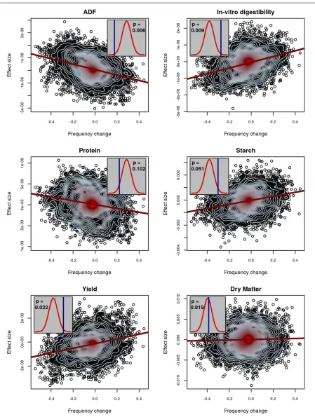
We reanalyzed data from a previous study that tested for selection in a decades-long breeding program for maize silage quality (Lorenz et al.2015). Very briefly, a selection index comprising experimentally measured traits related to silage quality was used to perform reciprocal recurrent selection for breeding improved maize. Traits composing the index in-cluded acid detergentfiber, protein content, starch content, in vitro digestibility, and yield (http://www.cornbreeding. wisc.edu). In total, 648 individuals from various stages of selection were genotyped. Between 240 and 300 of these individuals were also phenotyped, depending on the trait. Selection mapping was previously performed using simula-tions of drift to scan for selection, but the analysis did not identify any loci that showed significant evidence of selec-tion. This is despite quantifiable improvement of the popula-tion and demonstrated heritability of the index-composing traits (Lorenzet al.2015). We reanalyzed the same data to evaluate evidence for polygenic selection on the measured traits, which included NDF,in vitrodigestibility, crude pro-tein content, starch content, yield, and DM. Afterfiltering for
quality, but not MAF, these data consisted of 10,023 poly-morphic markers. Genomic prediction for these traits was generally effective (Figure S2). Due to the relatively small population size and recurrent selection breeding scheme, we expect slow LD decay and therefore for most of the ge-nome to be represented with this marker set. Further analysis of LD to determine the value of mind to use in our test for selection confirms this (Figure S3).
Figure 2 depicts the maize patterns of selection that were observed in our analysis. In these plots, the histogram shows the null distribution ofG^that was observed from a permuta-tion test, while the vertical line depicts the observed value of
^
Gwhen applied to the experimental data. We observed that, with the exception of protein, for the traits where we had ana priori expectation of selection, we not only identified that selection did occur, but we correctly estimated the direction of selection (positive or negative) from the data. One of the traits measured was silage DM, which was not a part of the selection index. We did not identify evidence of selection on DM, as was expected. To ensure that the existence of a single individual with a high breeding value does not lead to spuri-ous false positives, we reanalyzed the maize data after re-moving all SNPs with MAF,0.05. This did not lead to any appreciable change in the results (Figure S6).
Selection on chicken traits
We tested for evidence of selection in two panels of commer-cial lines of laying hens: one WL and one BL. Both closed lines have been selected over decades with a similar composite breeding goal which consisted of laying rate, body weight and feed efficiency, egg weight, and egg quality, among other objectives. The respective weights applied to the different traits varied between lines and over time. Traits analyzed included laying rate, egg weight, and breaking strength of eggs. Genotypes were available only for the postselection population, so initial allele frequencies were inferred based on pedigree data (Gengleret al.2007).mindwas determined based on separate evaluations of LD in the WL (Figure S4) and BL (Figure S5) populations.
Among the traits evaluated, we observed significant evi-dence of selection for increased laying rate in both WLs (P= 0.021) and BLs (P= 0.021). Tests were also suggestive of selection for increased eggshell-breaking strength in WLs (P,0.1; one-sidedP,0.05), while there was no evidence of directed selection for egg weight (Figure 3). To verify that these results were not driven by a small number of SNPs with high estimated effect sizes, we repeated the analysis with the 10 largest effect-size SNPs removed and saw virtually iden-tical results (Figure S7). The result for egg weight can be seen as a“negative control”since for this trait an optimum value is already achieved and maintained by stabilizing selection. The fact that we were not able to detect significant evidence of selection in a trait such as eggshell-breaking strength in both lines (although a tendency can be observed) may be due to the fact that improving those traits is part of a complex multi-objective breeding program, or simply that our test was
Table 2 Detection rate ofGbas simulation parameters vary
Parameter varied Tested values
No. individuals phenotyped 1000 500 250 100 50
Detection rate 1 0.99 0.83 0.4 0.21
Proportion of individuals selected 0.01 0.05 0.2 0.5 —
Detection rate 0.95 0.99 1.0 1.0 —
No. of generations of selection 100 50 20 10 1
Detection rate 0 0.81 1.0 1.0 0.18
Phenotyping generation 20 10 0 — —
Detection rate 1 1 0.86 — —
No. of generations postselection 5 20 50 100 —
Detection rate 1 1 0.26 0 —
Figure 3 Evidence of selection for chicken traits. For three traits in WL (left column) and BL (right column) hens, the relationship between estimated allelic effects at individual SNPs and the change in allele frequency over generations is plotted. The red line is a regression of effect size on allele-frequency change. Contour lines indicate the density of points, with blue contours indicating fewer points than red. Inset plots depict observed values of b
underpowered for these traits. The unavailability of experi-mentally estimated initial frequencies and our alternative use of pedigree-inferred initial allele frequencies likely weakened the power of the test as compared to the more complete data available for maize and in the simulations.
Discussion
We have defined a test statistic,G;^ that combines phenotypic and genotypic information to test for selection on traits con-trolled by many loci of small effect. The approach uses esti-mated effect sizes for individual loci and allele-frequency changes across two time points reflecting possible selection on those loci. Therefore,G^is most applicable in experimental or breeding populations, where both pieces of information are readily available via genotyping individuals from multiple generations. However, phenotypic information for estimating allelic effects is only required from a single time point, so this approach can be applied post hocusing DNA samples from previous generations even if phenotyping is no longer possi-ble. As the practice of sequencing ancient DNA from archeo-logical sites, museum samples, or other sources becomes progressively commonplace (Orlandoet al.2015), it will be interesting to explore whether or not this approach may prove applicable for ecological questions, evolutionary stud-ies, and for human research. However, simulations showed a decrease in power as the number of postselection generations increased, so there is a limit to how far back our test statistic can be fruitfully applied.
Powerful for highly quantitative traits
Methods for mapping genes associated with important traits or for identifying loci that are under selection are most power-ful for large-effect genes. A simple explanation for the disap-pointing number of associations that have been uncovered to date through GWAS is that complex traits are often controlled by many genes of small effect (Yanget al.2011). If this is the case, enormous sample sizes are required to map loci regard-less of the methodological enhancements that can be applied. Human geneticists have had success studying complex traits by using extremely large sample sizes (Rietveldet al.2013; Woodet al.2014). But, sample sizes of this magnitude are not yet achievable within resource limitations for most species and, arguably, will never be. Conversely, population-genetic studies aiming to scan for selection have been most success-ful at identifying hard sweeps, where a new mutation of large effect rapidly rises tofixation as a result of selection (Pritchardet al.2010). Only few methodologies with limited power exist for mapping soft sweeps, where the beneficial allele is already at an intermediate frequency at the start of selection (Garudet al.2015; Maet al.2015). A likely expla-nation for the presence of soft sweeps is that they often result from loci of small effect increasing in frequency slowly in a population and therefore existing on multiple distinct haplo-types or mutating multiple times beforefixation. In an agri-cultural context, many soft sweeps may be due to newly
defined breeding goals which put selection pressure on genes that were previously segregating in the populations, but were selectively neutral. TheG^ statistic does not attempt to map specific genes—instead it pools information from all SNPs to test for selection on specific traits. This approach completely avoids the question of which loci are associated with a trait. Instead of testing each SNP, we perform one test based on information from all SNPs. Therefore, a strong statistical sig-nal arises when a large proportion of SNPs behave similarly, but not when a few SNPs portray strong signals on their own. That said, researchers are often interested in identifying se-lected traits whether they correspond to selection on many genes at once or simply a few large-effect genes. In this case, the implementation of ourG^test in conjunction with a tradi-tional selection-mapping approach aimed at identifying se-lected loci will likely be powerful for identifying selection, regardless of the underlying genetic architecture (Figure 1). It was recently argued that most complex disease traits in humans are controlled by small-effect genes dispersed through-out the genome (Boyleet al.2017). Likewise, many important traits in agricultural animal and plant species tend to be quan-titative in nature and are presumably controlled by small-effect genes (Goddard and Hayes 2009; Wallace et al.2014). For these agricultural organisms, geneticists and breeders have long recognized the benefits that can be achieved by predicting breeding values and/or phenotypes based on models that use all SNPs simultaneously (Meuwissenet al.2001; Goddard and Hayes 2009; Heffneret al.2009). In fact, the development of these models has led to dramatic redesigns of modern breed-ing protocols (Schaeffer 2006; Cabrera-Bosquetet al.2012). TheG^statistic represents one avenue to leverage information from all measured SNPs to gain an understanding of the evo-lutionary history of a population. This approach is analogous to genomic selection/prediction, as used by animal and plant breeders, with an important distinction: instead of predicting breeding values to determine which individuals should be se-lected for the future, it uses genotypic frequencies over time coupled with phenotypic information to unravel the history of selection in the past.
Genotypes from the base population provide high power
allelic effects and/or allele-frequency changes are small, they cumulatively generate a powerful test since they can be com-pared across all genotyped loci. However, our analysis of the chicken data suggested that the power of the test can be re-duced through noisy estimation of allele-frequency change. Our reliance on pedigree data to derive initial allele frequen-cies was not as precise as the direct measurement of initial allele frequencies that was conducted for maize. Although we were still able tofind evidence of selection on traits including laying rate, which was almost certainly under the strongest selection; there were selected traits we did not detect, poten-tially because of this noise.
Future directions and conclusions
The use ofGbto test for selected traits avoids the require-ment of preliminarily identifying candidate genes or regions. Therefore, the approach is particularly applicable in experi-mental, agricultural, and natural populations for which avail-able resources dictate limited sample sizes for conducting massive mapping studies for such preliminary identification. In contrast to purely population-genetic analyses, which rely solely on genotypic information, the method requires that phenotypic data be collected from at least one time point of genotyped individuals. Additionally, two time points of ge-notypic information are needed, either directly or through pedigree-based imputation.
While the Gb statistic is most directly applicable for the discovery of traits that have been previously under selection during recent evolution, it may have additional applications. Recent studies have demonstrated that distinct physical re-gions of the genome, such as individual chromosomes, often contribute a disproportionate amount to trait variance (Bernardo and Thompson 2016). Rather than applying the b
G statistic genome wide, future research should be done to determine whether it can be applied across any collections of loci—such as individual chromosomes, pathways, gene fam-ilies, functional classes, or other categories—to test if these show evidence of selection on a quantitative trait. This would represent a process allowing researchers to map significant features as opposed to individual genes. Likewise, thus far we have estimated the direction of selection (positive or nega-tive) fromG;b but not the magnitude. Further research should be performed to determine whether or not this or a similar statistic can be used to recapitulate the selection gradient.
As it stands, usingbGsimply to identify traits that have been under selection in the past may prove enormously useful. Whether agricultural, experimental, or natural; it is often difficult to determine all of the traits that are advantageous in a population or that respond to natural or anthropogenic selection, including undesired selection responses. The appli-cation of thebGstatistic genome wide allows this determina-tion, which may help scientists select the right traits for maximum agricultural production, determine inadvertently selected laboratory traits affecting experimental outcomes, and establish ecologically important traits for survival in the wild.
Acknowledgments
We thank Natalia de Leon, Aaron Lorenz, and Lohmann for generating the maize and chicken biological data used in this study. We are grateful for helpful discussions with Emily Josephs and Aaron Lorenz. This research was supported by the U.S. Department of Agriculture–Agricultural Research Service, Current Research Information Systems project num-ber 5070-21000-038-00-D.
Literature Cited
Akey, J. M., 2009 Constructing genomic maps of positive selection in humans: where do we go from here? Genome Res. 19: 711– 722.https://doi.org/10.1101/gr.086652.108
Barsh, G. S., I. S. Farooqi, and S. O’Rahilly, 2000 Genetics of body-weight regulation. Nature 404: 644–651.https://doi.org/10.1038/35007519
Beissinger, T. M., L. Wang, K. Crosby, A. Durvasula, M. B. Hufford
et al., 2016 Recent demography drives changes in linked se-lection across the maize genome. Nat. Plants 2: 16084.https:// doi.org/10.1038/nplants.2016.84
Berg, J. J., and G. Coop, 2014 A population genetic signal of poly-genic adaptation. PLoS Genet. 10: e1004412.https://doi.org/ 10.1371/journal.pgen.1004412
Berg, J. J., X. Zhang, and G. Coop, 2017 Polygenic adaptation has impacted multiple anthropometric traits. bioRxiv 167551. DOI: https://doi.org/10.1101/167551.
Bernardo, R., and A. M. Thompson, 2016 Germplasm architecture revealed through chromosomal effects for quantitative traits in maize. Plant Genome 9.
Boyle, E. A., Y. I. Li, and J. K. Pritchard, 2017 An expanded view of complex traits: from polygenic to omnigenic. Cell 169: 1177– 1186.https://doi.org/10.1016/j.cell.2017.05.038
Browning, B. L., and S. R. Browning, 2009 A unified approach to genotype imputation and haplotype-phase inference for large data sets of trios and unrelated individuals. Am. J. Hum. Genet. 84: 210–223.https://doi.org/10.1016/j.ajhg.2009.01.005
Cabrera-Bosquet, L., J. Crossa, J. von Zitzewitz, M. D. Serret, and J. Luis Araus, 2012 High-throughput phenotyping and genomic se-lection: the frontiers of crop breeding ConvergeF. J. Integr. Plant Biol. 54: 312–320.https://doi.org/10.1111/j.1744-7909.2012.01116.x
de Los Campos, G., J. M. Hickey, R. Pong-Wong, H. D. Daetwyler, and M. P. L. Calus, 2013 Whole-genome regression and pre-diction methods applied to plant and animal breeding. Genetics 193: 327–345.https://doi.org/10.1534/genetics.112.143313
de Villemereuil, P., É. Frichot, É. Bazin, O. François, and O. E. Gaggiotti, 2014 Genome scan methods against more complex models: when and how much should we trust them? Mol. Ecol. 23: 2006–2019.https://doi.org/10.1111/mec.12705
Endelman, J. B., 2011 Ridge regression and other kernels for genomic selection with R package rrBLUP. Plant Genome 4: 250–255.https://doi.org/10.3835/plantgenome2011.08.0024
Evangelou, E., and J. P. A. Ioannidis, 2013 Meta-analysis methods for genome-wide association studies and beyond. Nat. Rev. Genet. 14: 379–389.https://doi.org/10.1038/nrg3472
Falconer, D. S., and T. F. C. Mackay, 1996 Introduction to Quan-titative Genetics. Pearson Education, Harlow, United Kingdom. Fisher, R. A., 1918 The correlation between relatives on the
suppo-sition of mendelian inheritance. Trans. R. Soc. Edinb. 52: 399–433.
https://doi.org/10.1017/S0080456800012163
Ganal, M. W., G. Durstewitz, A. Polley, A. Bérard, E. S. Buckler
Garrick, D. J., J. F. Taylor, and R. L. Fernando, 2009 Deregressing estimated breeding values and weighting information for geno-mic regression analyses. Genet. Sel. Evol. 41: 55. https://doi. org/10.1186/1297-9686-41-55
Garud, N. R., P. W. Messer, E. O. Buzbas, and D. A. Petrov, 2015 Recent selective sweeps in North American Drosophila melanogaster show signatures of soft sweeps. PLoS Genet. 11: e1005004.https://doi.org/10.1371/journal.pgen.1005004
Gengler, N., P. Mayeres, and M. Szydlowski, 2007 A simple method to approximate gene content in large pedigree popula-tions: application to the myostatin gene in dual-purpose Belgian Blue cattle. Anim. Int. J. Anim. Biosci. 1: 21–28. https://doi. org/10.1017/S1751731107392628
Gilmour, A. R., B. J. Gogel, B. R. Cullis, and R. Thompson, 2009 ASReml User Guide 3.0. VSN International Ltd, Hemel Hempstead, United Kingdom.
Goddard, M. E., and B. J. Hayes, 2009 Mapping genes for complex traits in domestic animals and their use in breeding programmes. Nat. Rev. Genet. 10: 381–391.https://doi.org/10.1038/nrg2575
Hansen, M. E., S. C. Hunt, R. C. Stone, K. Horvath, U. Herbiget al., 2016 Shorter telomere length in Europeans than in Africans due to polygenetic adaptation. Hum. Mol. Genet. 25: 2324–2330. Heffner, E. L., M. E. Sorrells, and J.-L. Jannink, 2009 Genomic
selection for crop improvement. Crop Sci. 49: 1–12. https:// doi.org/10.2135/cropsci2008.08.0512
Hufford, M. B., X. Xu, J. van Heerwaarden, T. Pyhäjärvi, J.-M. Chia
et al., 2012 Comparative population genomics of maize domes-tication and improvement. Nat. Genet. 44: 808–811.https://doi. org/10.1038/ng.2309
Kong, A., M. L. Frigge, G. Thorleifsson, H. Stefansson, A. I. Young
et al., 2017 Selection against variants in the genome associ-ated with educational attainment. Proc. Natl. Acad. Sci. USA 114: E727–E732.https://doi.org/10.1073/pnas.1612113114
Lawrie, D. S., P. W. Messer, R. Hershberg, and D. A. Petrov, 2013 Strong purifying selection at synonymous sites in D. melanogaster. PLoS Genet. 9: e1003527.https://doi.org/10.1371/journal.pgen.1003527
Lorenz, A. J., T. M. Beissinger, R. R. Silva, and N. de Leon, 2015 Selection for silage yield and composition did not affect genomic diversity within the Wisconsin quality synthetic maize population. G3 (Bethesda) 5: 541–549.
Ma, Y., X. Ding, S. Qanbari, S. Weigend, Q. Zhang et al., 2015 Properties of different selection signature statistics and a new strategy for combining them. Heredity 115: 426–436.
https://doi.org/10.1038/hdy.2015.42
Mathieson, I., I. Lazaridis, N. Rohland, S. Mallick, N. Pattersonet al., 2015 Genome-wide patterns of selection in 230 ancient Eurasians. Nature 528: 499–503.https://doi.org/10.1038/nature16152
Mathieson, I., S. Alpaslan-Roodenberg, C. Posth, A. Szécsényi-Nagy, N. Rohlandet al., 2018 The genomic history of Southeastern Europe. Nature 555: 197–203.
Meuwissen, T. H. E., B. J. Hayes, and M. E. Goddard, 2001 Prediction of total genetic value using genome-wide dense marker maps. Genetics 157: 1819–1829.
Orlando, L., M. T. P. Gilbert, and E. Willerslev, 2015 Reconstructing ancient genomes and epigenomes. Nat. Rev. Genet. 16: 395–408.
https://doi.org/10.1038/nrg3935
Plomin, R., C. M. A. Haworth, and O. S. P. Davis, 2009 Common disorders are quantitative traits. Nat. Rev. Genet. 10: 872–878.
https://doi.org/10.1038/nrg2670
Poland, J. A., P. J. Balint-Kurti, R. J. Wisser, R. C. Pratt, and R. J. Nelson, 2009 Shades of gray: the world of quantitative disease resistance. Trends Plant Sci. 14: 21–29.https://doi.org/10.1016/ j.tplants.2008.10.006
Pritchard, J. K., J. K. Pickrell, and G. Coop, 2010 The genetics of human adaptation: hard sweeps, soft sweeps, and polygenic adaptation. Curr. Biol. 20: R208–R215.https://doi.org/10.1016/ j.cub.2009.11.055
Qanbari, S., and H. Simianer, 2014 Mapping signatures of positive selection in the genome of livestock. Livest. Sci. 166: 133–143.
https://doi.org/10.1016/j.livsci.2014.05.003
Rietveld, C. A., S. E. Medland, J. Derringer, J. Yang, T. Eskoet al., 2013 GWAS of 126,559 individuals identifies genetic variants associated with educational attainment. Science 340: 1467– 1471.https://doi.org/10.1126/science.1235488
Sabeti, P. C., P. Varilly, B. Fry, J. Lohmueller, E. Hostetter et al., 2007 Genome-wide detection and characterization of positive selection in human populations. Nature 449: 913–918.https:// doi.org/10.1038/nature06250
Sargolzaei, M., and F. S. Schenkel, 2009 QMSim: a large-scale genome simulator for livestock. Bioinformatics 25: 680–681.
https://doi.org/10.1093/bioinformatics/btp045
Schaeffer, L. R., 2006 Strategy for applying genome-wide se-lection in dairy cattle. J. Anim. Breed. Genet. 123: 218–223.
https://doi.org/10.1111/j.1439-0388.2006.00595.x
Schweizer, R. M., B. M. vonHoldt, R. Harrigan, J. C. Knowles, M. Musianiet al., 2016 Genetic subdivision and candidate genes under selection in North American grey wolves. Mol. Ecol. 25: 380–402.https://doi.org/10.1111/mec.13364
Strandén, I., and O. F. Christensen, 2011 Allele coding in genomic evaluation. Genet. Sel. Evol. 43: 25. https://doi.org/10.1186/ 1297-9686-43-25
Strandén, I., and D. J. Garrick, 2009 Technical note: derivation of equivalent computing algorithms for genomic predictions and reliabilities of animal merit. J. Dairy Sci. 92: 2971–2975.
https://doi.org/10.3168/jds.2008-1929
Turchin, M. C., C. W. Chiang, C. D. Palmer, S. Sankararaman, D. Reichet al., 2012 Evidence of widespread selection on stand-ing variation in Europe at height-associated SNPs. Nat. Genet. 44: 1015–1019.https://doi.org/10.1038/ng.2368
VanRaden, P. M., 2008 Efficient methods to compute genomic predictions. J. Dairy Sci. 91: 4414–4423.https://doi.org/10.3168/ jds.2007-0980
Visscher, P. M., W. G. Hill, and N. R. Wray, 2008 Heritability in the genomics era —concepts and misconceptions. Nat. Rev. Genet. 9: 255–266.https://doi.org/10.1038/nrg2322
Wallace, J. G., S. J. Larsson, and E. S. Buckler, 2014 Entering the second century of maize quantitative genetics. Heredity 112: 30–38.https://doi.org/10.1038/hdy.2013.6
Weir, B. S., and C. C. Cockerham, 1984 Estimating F-statistics for the analysis of population structure. Evolution 38: 1358–1370. Wisser, R. J., S. C. Murray, J. M. Kolkman, H. Ceballos, and R. J. Nelson, 2008 Selection mapping of loci for quantitative dis-ease resistance in a diverse maize population. Genetics 180: 583–599.https://doi.org/10.1534/genetics.108.090118
Wood, A. R., T. Esko, J. Yang, S. Vedantam, T. H. Pers et al., 2014 Defining the role of common variation in the genomic and biological architecture of adult human height. Nat. Genet. 46: 1173–1186.https://doi.org/10.1038/ng.3097
Wright, S., 1937 The distribution of gene frequencies in popula-tions. Proc. Natl. Acad. Sci. USA 23: 307–320.https://doi.org/ 10.1073/pnas.23.6.307
Yang, J., B. Benyamin, B. P. McEvoy, S. Gordon, A. K. Henderset al., 2010 Common SNPs explain a large proportion of the heritability for human height. Nat. Genet. 42: 565–569. https://doi.org/ 10.1038/ng.608
Yang, J., S. H. Lee, M. E. Goddard, and P. M. Visscher, 2011 GCTA: a tool for genome-wide complex trait analysis. Am. J. Hum. Genet. 88: 76–82.https://doi.org/10.1016/j.ajhg.2010.11.011
Zeng, J., R. de Vlaming, Y. Wu, M. Robinson, L. Lloyd-Joneset al., 2017 Widespread signatures of negative selection in the ge-netic architecture of human complex traits. bioRxiv145755. DOI: https://doi.org/10.1101/145755.