Single frame super-resolution image system

University of Windsor University of Windsor

Scholarship at UWindsor

Scholarship at UWindsor

Electronic Theses and Dissertations Theses, Dissertations, and Major Papers

2010

Single frame super-resolution image system

Single frame super-resolution image system

Fei Yu

University of Windsor

Follow this and additional works at: https://scholar.uwindsor.ca/etd

Recommended Citation Recommended Citation

Yu, Fei, "Single frame super-resolution image system" (2010). Electronic Theses and Dissertations. 8214.

https://scholar.uwindsor.ca/etd/8214

This online database contains the full-text of PhD dissertations and Masters’ theses of University of Windsor students from 1954 forward. These documents are made available for personal study and research purposes only, in accordance with the Canadian Copyright Act and the Creative Commons license—CC BY-NC-ND (Attribution, Non-Commercial, No Derivative Works). Under this license, works must always be attributed to the copyright holder (original author), cannot be used for any commercial purposes, and may not be altered. Any other use would require the permission of the copyright holder. Students may inquire about withdrawing their dissertation and/or thesis from this database. For additional inquiries, please contact the repository administrator via email

Single Frame Super-Resolution Image System

by

FeiYu

A Thesis

Submitted to the Faculty of Graduate Studies

through Electrical Engineering

in Partial Fulfillment of the Requirements for

the Degree of Master of Applied Science at the

University of Windsor

Windsor, Ontario, Canada

2010

1*1

Published Heritage Branch

395 Wellington Street Ottawa ON K1A 0N4 Canada

Bibliotheque et Archives Canada

Direction du

Patrimoine de I'edition

395, rue Wellington Ottawa ON K1A 0N4 Canada

Your file Votre reference ISBN: 978-0-494-62719-8 Our file Notre reference ISBN: 978-0-494-62719-8

NOTICE: AVIS:

The author has granted a

non-exclusive license allowing Library and Archives Canada to reproduce, publish, archive, preserve, conserve, communicate to the public by

telecommunication or on the Internet, loan, distribute and sell theses

worldwide, for commercial or non-commercial purposes, in microform, paper, electronic and/or any other formats.

L'auteur a accorde une licence non exclusive permettant a la Bibliotheque et Archives Canada de reproduire, publier, archiver, sauvegarder, conserver, transmettre au public par telecommunication ou par I'lnternet, preter, distribuer et vendre des theses partout dans le monde, a des fins commerciales ou autres, sur support microforme, papier, electronique et/ou autres formats.

The author retains copyright ownership and moral rights in this thesis. Neither the thesis nor substantial extracts from it may be printed or otherwise reproduced without the author's permission.

L'auteur conserve la propriete du droit d'auteur et des droits moraux qui protege cette these. Ni la these ni des extraits substantiels de celle-ci ne doivent §tre imprimes ou autrement

reproduits sans son autorisation.

In compliance with the Canadian Privacy Act some supporting forms may have been removed from this thesis.

Conformement a la loi canadienne sur la protection de la vie privee, quelques

formulaires secondaires ont ete enleves de cette these.

While these forms may be included in the document page count, their removal does not represent any loss of content from the thesis.

Bien que ces formulaires aient inclus dans la pagination, il n'y aura aucun contenu manquant.

1*1

AUTHOR'S DECLARATION OF ORIGINALITY

I hereby certify that I am the sole author of this thesis and that no part of this thesis has

been published or submitted for publication.

I certify that, to the best of my knowledge, my thesis does not infringe upon anyone's

copyright nor violate any proprietary rights and that any ideas, techniques, quotations, or

any other material from the work of other people included in my thesis, published or

otherwise, are fully acknowledged in accordance with the standard referencing practices.

Furthermore, to the extent that I have included copyrighted material that surpasses the

bounds of fair dealing within the meaning of the Canada Copyright Act, I certify that I

have obtained a written permission from the copyright owner(s) to include such

material(s) in my thesis and have included copies of such copyright clearances to my

appendix.

I declare that this is a true copy of my thesis, including any final revisions, as approved

by my thesis committee and the Graduate Studies office, and that this thesis has not been

ABSTRACT

The estimation of some unknown quantity information from known observable

information can be viewed as a specific statistical process which needs an extra source of

information prediction strategy. In this regard, image super-resolution is an important

application.

In this thesis, we proposed a new image interpolation method based on Redundant

Discrete Wavelet Transform (RDWT) and self-adaptive processes in which edge

direction details are considered to solve single-frame image super-resolution task.

Information about sharp variations, both in horizontal and vertical directions derived

from wavelet transform sub-bands are considered, followed by detection and

modification of the aliasing part in the preliminary output in order to increase the visual

effect. By exploiting fundamental properties of images such as property of edge direction,

different parts of the source image are considered separately in order to predict the

vertical and horizontal details accurately, helping to consummate the whole framework in

reconstructing the high-resolution image.

Extensive tests of the proposed method show that both objective quality (PSNR) and

subjective quality are obviously improved compared to several other state-of-the-art

methods. And this work also leaved capacious space for further research, not only

theoretical but also practical. Some of the related research applications based on this

DEDICATION

ACKNOWLEDGEMENTS

There are several people who deserve my sincere gratitude for their great help.

First and foremost, I would like to give my sincere gratitude to my supervisor Dr.

Jonathan Wu for all of his generous support and guidance. His advice and irreplaceable

help, both academically and personally, have had, and will continue to have, a

tremendous impact on my life.

Faculty at the University of Windsor, including my committee members Dr. Mohammed

A. S. Khalid and Dr. Dan Wu from school of computer science are also those I am very

grateful to.

Also, I want to thank Ms. Andria Ballo (nee Turner) for her irreplaceable assistance and

cheerful conversation with me.

Moreover, I would like to offer great gratitude to Dr. Guanghui Wang and Mr. Michael

Chukwu for their sound technical advice and kind sharing of their opinions.

Finally, I must extend my most sincere love and gratitude to my parents, especially to my

Table of Contents

AUTHOR'S DECLARATION OF ORIGINALITY iii

ABSTRACT iv

DEDICATION v

ACKNOWLEDGEMENTS vi

LIST OF FIGURES ix

LIST OF TABLES xi

LIST OF ABBREVIATIONS xii

CHAPTER 1 INTRODUCTION 1

1.1 Problem Statement 1

1.2 Thesis Highlights and Contributions 3

1.3 Thesis Organization 4

CHAPTER 2 REVIEW OF STATE-OF-ART LITERATURES 5

2.1 Overview of SR Algorithms 5

2.2 Wavelet-Based SR Algorithms 8

CHAPTER 3 ANALYSIS OF WAVELET-BASED SR ALGORITHM 11

3.1 Wavelet Domain Edge Analysis 11

3.2 Wavelet Based Interpolation 13

3.2.1. Discrete Wavelet Transform (DWT) 13

3.2.2. Redundant Discrete Wavelet Transform (RDWT) 13

3.2.3. Inverse Discrete Wavelet Transform (IDWT) 15

CHAPTER 4 PROPOSED ALGORITHMS 18

4.1 Proposed Edge-Adaptive SR Algorithm 18

4.1.1 Preprocessing 18

4.1.2 Super-resolution Realization 20

4.1.3 Aliasing Processing & Feature Constrain 23

4.1.4 IDWT Implementation 24

4.2 Other Related Applications 25

4.2.1 Foreground Extraction 25

4.2.2 Change Detection 26

CHAPTER 5 EXPERIMENT RESULTS AND DISCUSSION 28

5.1 Experimental Results of the Proposed SR Algorithm 28

5.2 Experimental Results of the Proposed Foreground Extraction Algorithm 50

5.3 Experimental Results of the Proposed Change Detection Algorithm 51

CHAPTER 6 CONCLUSIONS AND FUTURE WORK 54

6.1 Conclusions 54

6.2 Future Work 55

REFERENCES 56

V I T A A U C T O R I S 60

LIST OF FIGURES

Figure 1 Single-frame image resolution enhancement example (resolution 64

x 64—256 x 256) 2

Figure 2 Relationship between HR and single LR 6

Figure 3 Digitized image containing edge information 11

Figure 4 Redundant DWT decomposition of image 14

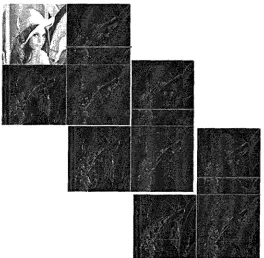
Figure 5 Redundant DWT decomposition of Lena (512x512-*1024xl024)... 14

Figure 6 IDWT sketch of Lena (4X512X512—1024X1024) 15

Figure 7 Sample of aliasing 16

Figure 8 Sample of aliasing using Barbara as input 17

Figure 9 Decomposition of input image (using Lena as an example) 19

Figure 10 Scale and magnitude propagation analysis (using Lena as an

example) 22

Figure 11 Horizontal growth rate propagation (other direction similar) 22

Figure 12 IDWT sketch of Lena (4x512X512—1024X1024) 24

Figure 13 Two different input frames changes generation 27

Figure 14 Example of the subjective judgment of SR outputs (Top: original;

down left: good output; down right: bad output) 28

Figure 15 SR outputs using Lena as input (a: original; b: down-sized image; c:

proposed SR result; d: zero-padding SR result) 31

Figure 16 SR outputs using Boat as input (a: original; b: down-sized image; c:

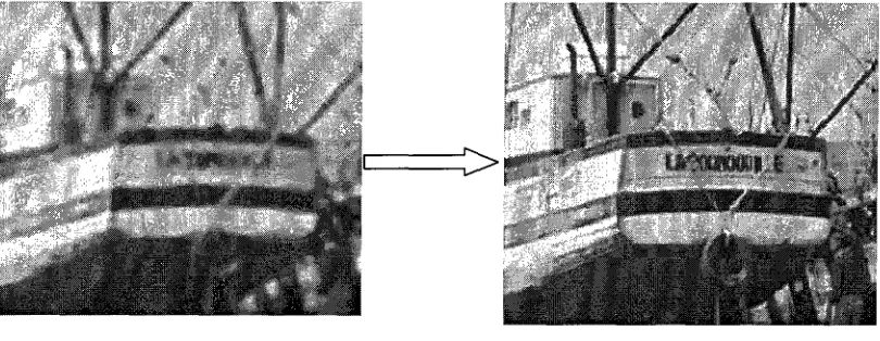
proposed SR result; d: zero-padding SR result) 33

Figure 17 SR outputs using Bridge as input (a: original; b: down-sized image;

c: proposed SR result; d: zero-padding SR result) 35

Figure 18 SR outputs using Peppers as input (a: original; b: down-sized

Figure 19 SR outputs using Barbara as input (a: original; b: down-sized

image; c: proposed SR result; d: zero-padding SR result) 39

Figure 20 SR outputs using Baboon as input (a: original; b: down-sized image;

c: proposed SR result; d: zero-padding SR result) 41

Figure 21 SR outputs using Airplane as input (a: original; b: down-sized

image; c: proposed SR result; d: zero-padding SR result) 43

Figure 22 SR outputs using Elaine as input (a: original; b: down-sized image;

c: proposed SR result; d: zero-padding SR result) 45

Figure 23 Detail from Proposed and Zero-padding SR outputs (for each

group, the front one is from proposed SR, the latter is from zero-padding) ..47

Figure 24 Results of proposed foreground extraction algorithm (left: original

images, right: outputs) ....• 51

Figure 25 Results of proposed change detection algorithm (top two: original

input images, down: different outputs) 53

LIST OF TABLES

Table 1 CDF 9/7 Coefficients 19

Table 2 Simulation PSNR Results for Proposed SR and Standard SR (image

size: 256 X 256-^512 X 512) 48

Table 3 Simulation PSNR Results for Proposed SR and State-of-art SR

LIST OF ABBREVIATIONS

SR: Super Resolution

HR: High Resolution

LR: Low Resolution

PSNR: Peak Signal to Noise Ratio

RDWT: Redundant Discrete Wavelet Transform

DWT: Discrete Wavelet Transform

IDWT: Inverse Discrete Wavelet Transform

PC A: Principal Component Analysis

HMT: Hidden Markov Tree

MLP: Multilayer Perception

CDF: Cohen-Daubechies-Feauveau

MSE: Mean Square Error

dB: decibel units

HD: High Definition

CHAPTER 1

INTRODUCTION

1.1 Problem Statement

As one of the most important information carriers in modern life, images have

irreplaceable positions in many areas. With the development of modern image processing

technology and increasing computational power, we can overview many classic

algorithms from a time-consuming point of view. Among them, pursuing high-resolution

(HR) or Super-resolution (SR) images is always a difficult, though very important task.

The requirements of HR exists not only in daily life (i.e. entertainment, surveillance,

media, medical area), but also in national defense, remote sensing and communication,

and so many other areas.

Normally, we can choose hardware artifices to fulfill this task by reducing the pixel size

when manufacturing optical instruments. However, it is well known that there exists

optical limitations within unit pixel size, and ignoring that will engender shot noise and

exponentially increase the device price. Thus, people try to solve this problem from a

software point of view. Being more specific, from a signal processing point of view,

image resolution up-conversion is a process focusing on the up-sampling of the already

digitally sampled signal; while from an image processing point of view, increasing the

resolution of an image is a process which generates or recovers a higher resolution image

from one or more low resolution image resources. Both sides present a significant

challenge because of the uncertainty of the original source.

Single-frame input and multi-frame input are two situations we face when trying to

video) which have different sub-pixel shifts, and each of them contain highly-related

information (i.e. relative scene motions) which can be exploited to obtain a SR image [1].

However, most of the time, we do not have enough related input image sources at hand.

This requires us to develop the algorithm based on single-frame input SR, meaning the

input source is a single raster image. In other words, the single-frame SR is also known as

image scaling, interpolation, zooming and enlargement [2]. The requirement of solving

such a single frame image super-resolution problem arises in several practical situations

[5]. In investigative criminology for example, we always face the problem that one has

available face and fingerprint databases but only a single observation for the suspect.

That specific given low resolution (LR) image may be used to generate the very HR

image we need with no other related information provided. Similarly, a situation can be

found when a particular LR text image is enhanced to generate HR images. We can see

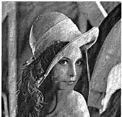
an example of single frame image resolution enhancement from Figure 1.

Resolution = 64 x 64 Resolution = 256 x 256

1.2 Thesis Highlights and Contributions

This thesis presents a general investigation on the main classification of single-frame

image super-resolution algorithms and proposes a novel proposed SR algorithm based on

the combination of redundant discrete wavelet transform (RDWT), edge-adaptive and

aliasing removal strategies. Lots of input images are used in the proposed design to

assure the robustness of the algorithm. And by using the proposed system, we try to solve

the main challenges in traditional SR problems, which are to find a way to blur,

de-noise and de-alias way so as to increase spatial resolution.

The principle advantage of this scheme lies in its high efficiency and stability in various

kinds of images. The outputs show obvious improvement on the performance of the

existing techniques. Though the proposed algorithm is derived from the ideas of some

core functionalities found in some existing research, the improvement of the whole

system constrains the feasible solutions for the prediction of the unknown coefficients.

In addition, since the whole system is modularized and every part can be substituted by

more flexible or more advanced algorithms, there will be plenty of spaces left for

modification in order to extend the capability. Some of the potential changes will be

discussed later in this thesis as well, so that those who are interested will have the benefit

1.3 Thesis Organization

The thesis begins with a general overview of the image super-resolution conception and

classification followed by the motivation and challenges in the single-frame

super-resolution mission. Contributions and brief discussions of this work are also provided.

Chapter 2 gives a review of the history of the development of super-resolution methods.

State-of-art literature is reviewed in order to follow the classification of the strategy used

in each work.

Chapter 3 is focused on the introduction of the main principal of all conceptions which

are used in the proposed algorithms. We explain edge modeling, wavelet-based

interpolation, aliasing detection and rectification using mathematical methods and other

image processing techniques.

Chapter 4 initially introduces the details about the proposed single-frame SR algorithm,

following the order of the whole system, which can be divided into parts like

preprocessing, super-resolution and analysis, and the detection and correction of the

potential aliasing areas. At the same time, some of the related applications are briefly

introduced; for example, image changing detection and foreground extraction, including

the principle and the flows of the proposed algorithms are examined.

Chapter 5 shows the standard which is used to judge the SR algorithms and the detailed

experimental data of the experiment on the proposed algorithm. Then the experimental

results for the real images are shown followed by the analysis of the result and the

comparison of the outputs between the proposed algorithm and the state-of-art literature.

Also, the outputs of the related algorithms such as image foreground extraction and

changing detection are shown as well.

Chapter 6 gives a summary of contributions and conclusions presented in this work,

followed by a prospect for future work.

CHAPTER 2

REVIEW OF STATE-OF-ART LITERATURES

2.1 Overview of SR Algorithms

As the importance of SR in the image processing area is so obvious, there are lots of SR

methods and surveys on those methods in research literature. Among them, many

significant surveys [2] [3] [4] [5] [6] can be used to start with our study in this classical

area. Though they all have their own points of emphasis on different kinds of algorithms,

the main clue they try to exploit is the strategy to solve the specific tasks in SR

reconstruction techniques which are de-blurring, de-noising, and alias removal, and the

comparison of the effects from the experiment outputs.

In general, the SR algorithms can be divided into two groups: reconstruction-based and

learning-based [5]. When we mention reconstruction-based SR, in most cases, we have to

find a way to recover a HR image from several LR observations. To do this some cues

are always needed, in order to find the relationship between those LR inputs. Based on

motion cues much existing literature examines sub-pixel shifts among the different LR

images in order to find a clue with which to interpolate them onto a HR grid. This is

followed by restoration to remove blur and noise. According to [1], there are multiple

studies from both time domain and frequency approaches. As for learning-based SR

algorithms, a database of several other similar images is needed in order to find a prior on

the original HR image. Among them, neural network is a good instrument for users to

find a stable relationship between each input [1]. However, as these methods always

require multiple inputs, we will discuss more about single-input algorithms in the

As for still image SR algorithms, we classify them into global and local items [5]. There

is a model of the relationship between a HR image and single-input image as shown in

Figure 2.

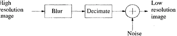
High resolution

image Blur Decimate

Low „«. resolution y image T Noise

Figure 2 Relationship between HR and single LR

Illuminated by [8], the Papoulis-Gerchberg method [7] is an example of global

approaches in which the input LR image is considered to be a single entity for processing.

The main idea is that if the measurements of the object spectrum are nearly noise free,

then the entire spectrum of the object can be generated uniquely using the principle of

analytic continuation. This is a good idea in both single and multiple input situations;

however, the result cannot be controlled well if the noise is obvious. Principal component

analysis (PCA) -based global learning method for super-resolution reconstruction [4] [9]

is a global learning method, which tries to obtain a few significant eigenimages of a

database of several similar HR images. The characteristic of these eigenimages are then

be used to compute the coefficients needed for up-sampling the LR image. However, this

kind of method suffers from the infection of the blur existing in the input. Consequently,

the associated eigen expansion between blur LR image and the related HR database will

be very poor in producing the ideal HR image. And the detail of the image, for example

edge, is independent within the database and is hard to spread follow the eigen expansion.

Local SR approaches are good choices for the consideration of edge details. We can start

from Kernel SR algorithms which are amply discussed in [2]. A basic function is needed

to approximate the continuous function needed to underlying the discrete samples that

make up the HR image. As is well known to all, linear and cubic kernels can be used

the convenient of kernel calculation. The idea in [10] is a method trying to divide the

pixels into classes like flat and edge areas, and then treat them separately when doing the

enlargement. The idea of adding weight from different direction of the details is a good

start. [12] is similar to this because each pixel belongs to a single class instead of multiple

classes. Neural network can be used in local method as well [11]. Pixels consists of the

around the source pixel in the local window are used as the input for the neural network,

and the neural network can be trained by using a decimated image as input and the

corresponding original image as target in order to get the output consists of the pixels

needed for the super-resolved image. Sparse derivative is used in [13] which attempts to

use the distribution of the derivative of natural images as a model to exploit SR image.

One of the advantages of using local approaches is that the edge information can be

properly reserved. When dealing with a noisy source, it is necessary to present a smart

interpolation way by anisotropic diffusion in order to sharpen edges and generate

plausible detail [14] [15]. This strategy may show a smooth effect around the edge area,

however, distortion is unavoidable. Xin Li produced similar work in [16] called new

edge-directed interpolation, by using the duality between the low resolution and high

resolution covariance for SR processing. He found a clue between the covariance of

neighboring pixels in local windows around the LR source and those in the HR target.

Direction of diagonal neighbors are considered in the first pass, followed by the second

pass, which uses horizontal and vertical neighbors to interpolate the rest of the pixels. In

[17] we can find a locally-adaptive zooming algorithm which is set point on

discontinuities and sharp luminance variations while doubling the LR source in

horizontal and vertical directions. All of them make good use of local edge information to

predict the detailed local areas in the output HR image. This is a great direction of

2.2 Wavelet-Based SR Algorithms

Wavelet-based SR algorithms are unique and irreplaceable contributions in all kinds of

SR algorithms, and we can find the discussions about the merits and pitfalls of different

kinds of wavelet-based SR algorithms in almost all good surveys in SR area; for example

in [l]-[6] [18] [19]. Analysis LR from a wavelet point of view gives us a better

understanding of the possibility of increasing the resolution of signal and the possibility

of using all kinds of wavelet instruments which have proved to be good at forecasting

tasks; instead of simply using traditional image enhancement strategies. Multi-resolution

analysis of the input signal is widely used and has proved to be powerful in

wavelet-based SR areas because the signal structure similarity across the scales of the

decomposed LR source can be found to predict the next higher fine scale of detail

coefficients. However, there are divergences of approach occurring in the method of

prediction.

Hidden Markov Tree (HMT) has been widely used in wavelet processing areas. [20] sets

up a method using HMT to predict the next set of coefficients using training data. This

has shown better HR results than traditional interpolation algorithms such as bilinear ones.

[21] follows the same clue but makes some additional modifications by eliminating the

requirement for training and simplifying the coefficient sign prediction method. These

two methods are computationally efficient, and the quad-tree they propagated is the

magnitude the parents coefficients to the child level, which yields unpredictable results.

Neural network can be well used in wavelet SR as well [23]. Multilayer perception (MLP)

interpolation schemes based on the wavelet transformation and sub-band filtering are

proposed [23]. The sub LR image signal can be viewed separately, and then the MLP

progress is used to predict the corresponding coefficients needed in the related HR image.

As the wavelet analysis/synthesis procedure and MLP procedure can be implemented

easily by using VLSI techniques, this kind of methods can be implemented on hardware

as well. However, the veracity of the output is fair, and the system is not that stable and

may yield distortion if the source is not well selected.

Like traditional SR algorithms, local details such as edge information are still a very

important direction which has been extensively studied and used. Directional wavelet

filtering has been used in [22] to ensure the effect of the output in the direction of the

detail edges. Multiple and flexible directional filtering is used to model the characteristics

of the target image edges. Though performing well on complex LR images, [22] provides

marginal gains in less complex ones. Markov Chain Monte Carlo is widely used in

wavelet analysis and has also been used in [24] to synthesize a system which is edgily

adaptive.

There is a special family of wavelet-transform modulus which tries to maximize

capturing the sharp variation points of signals. Then it tries to follow the local Lipschitz

regularity across the scales, which characterizes [25] [26] [27]. This is one of the most

important instruments we use in our proposed algorithms, and we will specifically

discuss this later. Grace et al. attempt to extend this work into the single-frame image SR

area by [28], and then they consolidate their work in [29]. From a spatial point of view,

they proposed an algorithm which uses wavelets to extract sharp variations in the LR

image and use this information to adapt to the image to local singularity characteristics.

This strategy, though suffering from high complexity, yields sharper images in the output.

Edge information, which is very important in SR area, is well protected to a great extent.

The visual quality of the output images is not sensitive to the accuracy of the model,

making the whole system robust. However, aliasing still seems to be a key problem they

face judging from the visual effect.

Another class of local approaches we would like to supplement here is SR through the

local linear embedding in contourlet domain. It is similar to wavelet-based SR algorithms;

and also, it is further capable of capturing the smoothness along contours making use of

directional decompositions [5] [30] [31]. A set of high resolutions have been trained

locally in order to get the information we need to predict the contourlet coefficients at the

action is performed later using the learnt coefficients which recover the super-resolved

image. In effect, we can tell from the output of their experiment that edge information

can be well protected by using the high resolution representation of an oriented edge

primitive from the training data, while the use of wavelets alone can only allow us to

capture horizontal and vertical edges properly. Normally, because the training set may

have different average brightness values, the contourlet coefficients in all subbands,

except at the lowpass subband where we obtain the contourlet coefficients, should be

acquired from a suitably interpolated version of the LR image [32]. This will cause a time

consuming burden and cannot avoid the transference of the aliasing effect as well.

On the whole, all these unique works we introduced here suffer from several drawbacks

from some perspectives, yet provided great and promising paths and ideas for us to

explore for our proposed system.

ANALYSIS OF WAVELET-BASED SR ALGORITHM

3.1 Wavelet Domain Edge Analysis

Edge can be described as a form of information in the spatial domain and wavelet domain,

which is used to do image processing or signal processing. It is helpful in the whole

image modeling process, as well as in handling detailed parts of the images, where the

most important information may be found. By studying the changes in the neighborhood

of the edges, it may be possible to find a useful changing disciplinarian which can used to

predict whole images or entire singles.

Starting with a brief overview of edge performance in the spatial domain will give us a

clear understanding of the changes they cause in continuous space. There are two key

observations we focus on: a sharp transition of the image intensity, which happens across

the edge orientation and the image intensity field, which is almost uniform when we

follow the same side of the edge orientation [33]. With these properties, we can easily

track the changes of the information when we digitize the image intensity field into data

arrays. By checking the example in Figure 3 [33] below, there is a clearer sense about

what we are trying to explain here. It is obvious that the local gradient and the rate of

change in itself when doing down-sampling is where we should keep our emphasis on.

A similar situation happens in the wavelet domain as well. By using decimated wavelet

transforms with equal decimation rationing along the horizontal, vertical, and diagonal

directions, we can trace the geometric constraint as we explained in the spatial domain,

not to mention if a linear non-decimated wavelet is used. By tracing the changes of the

wavelet transform along different levels, and due to the frequency aliasing introduced by

the decimation, the edge information can be easily located.

To extend the work in [25] [26] [27], which tries to maximize capturing the sharp

variation points of signals, and then tries to follow the local Lipschitz regularity across

the scales characterizes what we mentioned in the last chapter where we explained the

wavelet framework as follows [29].

In multi-scale wavelet domain, we normally trace information along scale "s" to

determine the global or local nature of the signal features. At the scale "s", the wavelet

transform of a signal wsf(x), which is defined as the following function (1), can be

viewed as the first derivative of f *0S, while an extremum of small magnitude indicates a

region of relatively slow variation. It is useful to locate the sharp transition regions.

W r f ( x ) = f ( x ) . ( s ^ ) ) = sA(f.9.)(x) (1)

w n e r eesfx\ = IefiL>| is a smooth function integrates to 1 and converges to zero at infinity.

To further explain and make it more common, if 9s is Gaussian, the detection of local

extrema corresponds to the well known Canny edge detector [34].

Extending (1) into two dimensions, we have ws'f(x,y) and ws2f(x,y) for the wavelet

transform of f(x), we have the local maximum at the greatest gradient as shown in

equation (2), which indicates the edge information locally.

Wsf(x,y) = ^|Ws,f(x,y)|2+|Ws2f(x,y)|2 (2)

3.2 Wavelet Based Interpolation

3.2.1. Discrete Wavelet Transform (DWT)

The defined problem within the context of wavelet inspired techniques is modeled after

the prediction of the unavailable higher detail wavelet coefficients. The discrete wavelet

transformation is well proven to be a good way to deal with interpolation problem which

uses low-pass and high-pass filters, h(n) andg(n), to expand a digital signal. They are

referred to as analysis filters. After DWT, the coefficients Ck (coarse coefficients) and dk

(detail coefficients) are produced by convolving the digital signal with each filter and

then decimating the output. Coarse coefficients provide information about low

frequencies, while detail coefficients provide information about high frequencies. Most

existing DWT-based algorithms focus on predicting the needed high coefficients in order

to synthesize the high-resolution image.

3.2.2. Redundant Discrete Wavelet Transform (RDWT)

To generate a A:-times larger size image than the original image with maximum image

details such as edges, corners etc. are the fundamental concept of the image interpolation.

As mentioned, we focus on generating a noise-free, blur-free, and alias-free interpolation

algorithm, which means we need as much input information as possible to solve this

ill-posed problem.

The use of decimators makes the DWT more computationally efficient by ignoring

redundant coefficients. However, these coefficients may be potentially very valuable

information needed in the reconstruction process (reducing aliasing, etc.). For the

consideration of this it is beneficial to remove the decimators. That is why we use RDWT

in this proposed algorithm, and the process of RDWT is shown in Figure 1 where the

original image can be divided into the approximation part, the horizontal details, the

vertical details and the diagonal details. In the decomposition structure of the 2-D RDWT,

is an example of the RDWT shown in Figure 1, a 512x512 image will generate one

512x512 coarse sub-image and three 512x512 detail ones after RDWT, which is

1024x1024 values, that is obviously much more than 512x512 after DWT.

Input Image

— •

Low Pass

1 — • High Pass — • — • Low Pass High Pass Low Pass High Pass ->• App. coars Hor. detail Ver. detail Dia. detail

£>FfT(.s;.9(D4)) a

i i4 m - - 4 » t + li" ' 4 M 4 - 2i"i4 m + 3 i i4 > « + 4 ^^im+l ry+ i ...rv'+1 , " 4 m + 1 2 " 4 m + 1 5

~"*16m--16m-i-r " " I S r a + l S

zszisr_zs

Q /+ 2 •••QJ- QJ*2 ...CV+ 2

a i1 6 m + 4 S — 1 6 » + 6 3

Figure 4 Redundant DWT decomposition of image

Figure 5 Redundant DWT decomposition of Lena (512x512-^1024x1024)

3.2.3. Inverse Discrete Wavelet Transform (IDWT)

In order to do interpolation, which is up-sampling in the wavelet domain in a sense, we

have to know the detailed information in vertical, horizontal, and diagonal directions.

Furthermore, we have to do an inverse calculation of the process shown in Figure 4 and 5

(up sample process needed after each filter), which means we need the information about

the one coarse part and three detailed parts of the target image. The prediction of the

detailed information section is explained in the following chapters as implementation

details. As long as we have all the information we want, IDWT will be done to get the

HR image we need. Figure 6 is a sketch map on Lena for IDWT. It is sample produced by

deciding where original size 512x512 image will be enlarged to size 1024x1024.

Theoretically, any size of interpolation can be achieved by using this strategy.

Figure 6 IDWT sketch of Lena (4*512x512->1024xl024)

3.3 Aliasing Areas Analysis

As defined in digital processing area, in signal processing and related disciplines, aliasing

refers to an effect that causes different signals to become indistinguishable from each

other (or aliases of one another) when sampled. It also refers to the distortion or artifact

those results when the signal reconstructed from samples is different than the original

continuous signal. Functions whose frequency content is bounded (band limited) have

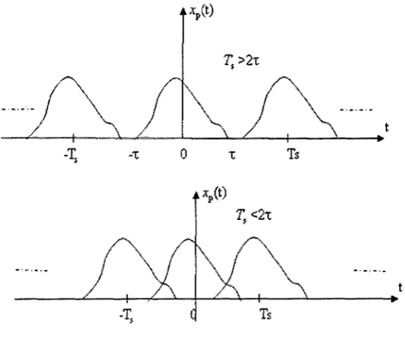
the original function can be perfectly reconstructed from the infinite set of samples in theory. Figure 7 is a sample of non-aliasing and aliasing situation.

• *p<B

Figure 7 Sample of aliasing

As in the SR area, original images can be viewed as an already down-sampled single

which will undoubtedly contain areas of aliasing. Those areas will provide distortion

which completely erodes the inter-scale dependency of the coefficients. If this

phenomenon is ignored, the effect will pass along on the aliased image pixels resulting in

the degeneration of the estimated higher resolution outputs. Figure 8 is an example using

the image Barbara as input. We can find significant aliasing along the headband of the

woman on the right image compared to the original one on the left. Therefore, we need a

method to efficiently extract the aliasing areas of the original image and handle those

separately. Since aliasing may have reaction in both the time and frequency domains, it

can be analysis separately to increase the accuracy.

In the frequency domain, high magnitude coefficients with a corresponding high decay

rate will indicate an inadequate sampling rate and possible aliasing. This can be tested by

tracing the wavelet changes along different scales while doing decompositions. While in

the time domain, areas of the images with singularities and edges at the same rate as the

image spatial resolution can be potential aliasing areas.

Though the potential aliasing areas are fairly complex to accurately estimate in a SR

system, they do need to be accurately detected and properly and separately handled while

doing predictions, before the IDWT, in order to increase the veracity of the output HR

CHAPTER 4

PROPOSED ALGORITHMS

4.1 Proposed Edge-Adaptive SR Algorithm

4.1.1 Preprocessing

As discussed by Nyquist & Shannon, we face an ill-posed question because if we define

the HR image as the target signal. As we only have one low-resolution image as input,

which is part of the original signal, it is not possible to recover the whole original signal

(especially the detail high frequency parts already ignored). In order to fulfill the task

which relies on a single input LR image to generate a HR output image, we decided to

use the wavelet method mentioned before. Some ideas derive from the core

functionalities of the existing methods we mentioned in the previous chapters; however,

we focus on the definitive model that constrains the feasible solutions for the prediction

of the coefficients.

To begin with, the input image is decomposed by RDWT, which is an over-complete

representation of the coefficients at each scale. The benefit of using RDWT has been

discussed before, giving us additional information for solving linear equations later.

Moreover, by using RDWT one can obtain L DWT results by only decomposing an

L-length signal x(k) and its one step shift, instead of decomposing each shift of x(k)

respectively. Alternatively we can say that this redundancy provides flexibility and

compatibility for more stability and robustness. [35].

The Cohen-Daubechies-Feauveau (CDF) 9/7 bi-orthogonal symmetric wavelets, which

are well used in JEPG 2000 lossy compression, is used throughout the wavelet

multi-resolution analysis and synthesis progress. CDF 9/7 share properties that all generators

and wavelets in this family are symmetric. This fact is used to ensure the robustness of

the decomposition and reconstruction process. The detailed coefficients of the CDF 9/7

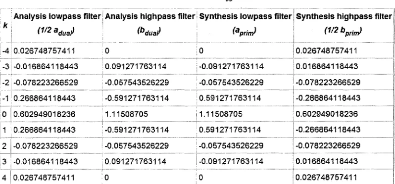
wavelet is given in Table 1 [36].

Table 1 CDF 9/7 Coefficients

! Analysis lowpass filter Analysis highpass

-4 0.026748757411 -3 -0.016864118443 -2 -0.078223266529 -1 0.266864118443 0 0.602949018236 1 0.266864118443 2 -0.078223266529 3 -0.016864118443 4 0.026748757411 0 i 0.091271763114 -0.057543526229 -0.591271763114 1.11508705 ;-0.591271763114 I -0.057543526229 0.091271763114 0

filter} Synthesis lowpass filter

'apriny

jo | -0.091271763114 I -0.057543526229 10.591271763114 11.11508705 j 0.591271763114 | -0.057543526229 1-0.091271763114 jo

Synthesis highpass filter

0.026748757411 0.016864118443 -0.078223266529 -0.266864118443 0.602949018236 -0.266864118443 -0.078223266529 0.016864118443 0.026748757411

In order to ensure the comparability of the results, we keep the source image as the

original one, and down sample the image using CDF 9/7-based DWT to reduce that into

half of the size. Then, the downsized image is used as the input image and decomposed

into different scales (see Figure 9).

Information of different scales (so, Si, S2 ...) is saved separately according to the scale

they belong to, and that information is classified into three sorts: horizontal, vertical, and

diagonal. Since various kind of images have different information in different directions

(e.g. horizontal details (Boats) and vertical details (Peppers)), and different weighting

strategies can be realized within different sorts.

4.1.2 Super-resolution Realization

It is well known that feature information is always important in image processing.

Finding sharp variations (e.g. we use the Canny edge detector to find a local maximum)

is the way we can use to obtain edge information. Many previous studies, as previously

discussed, show that a multi-scale edge characterization framework is a convenient

analysis of edges in the wavelet domain which is used here as well. In this section and the

next, we first present the mathematical process of the proposed edge-adaptive algorithm

and then describe the process of IDWT.

Starting with wavelet multi-resolution approximation modeling, we may find that there is

a conjunction function/, of which there is an orthogonal projection at the scale s (2J) on

space Wj. The approximation between two continuous scales s (2J) and s-1 (2J"') are

respectively equal to their projections on the two consecutive spaces, that is Wj and Wj.].

Moreover, we can find some relationship between these two spaces by the expression of

the following equation 3.

WJ-I = W J © V J ( 3 )

where Vj is the passing orthogonal factor of Wj in Wj.]. Hence, the projection function f

can be the combination of projections on Wj and Vj. Furthermore, Vj contains the detailed

information of the projection on the next space, i.e. Vj.i, which cannot be found in the

source space Vj. Based on the wavelet decomposition analysis, we can trace this

orthogonal projection of iteration through the following equation 4, and get the

information we needed throughout the wavelet analysis.

Wj = Wj + .©Vj + i ( 4 )

This makes the process like a regression which has some relationship linked by specific

coefficients between each other, and it is our job to use some mathematics parameters to

unfurl this relationship. The Lipschitz Exponent is the one we choose [26] [27].

In particular, for the convenience of computation on the singularity problem shown in

equation 2 before, we introduce Lipschitz Exponent a . A function f (x) is uniformly

Lipschitz a over an interval (a,b) if and only if there exists a constant K > 0 such that

for all x e (a,b), the wavelet transform satisfies equation 5 [28].

|Wsf(x)|<Ksa

I V ; | (5)

In this case, if we assume the conjunction function f between the two continues space Wj

and Wj.i is uniformly lipschitz, then the two projections, i.e. Vj and Vj_i are linearly

related too, as shown in equation 6.

VjOcT.Vj-i (6)

As we focus on the local Lipschitz parameters of the difficult singularities, the task of

estimating the details in scale 0 is equivalent to find ^m and am as shown in equation 7.

W2'f[x^] = Km(2J)a™, j=l,..J (7)

To recover Km and ocm in equation 7, we only need to solve the following linear

regression equation 8.

log 2 (W2J f [ x » ]) = log 2Km + jet-,, j=l,..., J (8)

As long as we use RDWT in the preprocessing process, and have plenty of

high-resolution classified information, we can obtain the Lipschitz parameters from the above

equations, and the decay rate instead is considered. We then calculated the absolute

maximum value of the coefficients. The slope of the log 2 between the coefficient and the

absolute value of the coefficient in the same position in the next higher scale is the

assuming that si and so have the same coarse components, we have sufficient

information for the reconstruction of the high-resolution image.

Magnitude

Figure 10 Scale and magnitude propagation analysis (using Lena as an example)

-v/p^saa

S

1 - - -p

':•!'

& "

->*3

\ - i

»* J

• 1 l i

i—& £~h xsa

4.1.3 Aliasing Processing & Feature Constrain

As discussed before, we can detect the potential aliasing areas through both frequency

and time domains, which jointly provide an excellent indication of aliasing in the original

input image. In the time domain, the expression is a high pass operator dealing with the

inter-pixel singularities and edges information, while in the frequency domain, we focus

on those areas with high magnitudes as well as a high decay rate. After dealing with both

of these domains, all those areas which have been defined as potential aliasing areas are

excluded from the extrapolation and processed separately, and as in our case, are padded

with zero values in the unavailable scale which needs to be predicted.

To make the whole algorithm more robust for all kinds of images, the predicted

coefficients are classified into bounded and unbounded variations [37] [38] based on the

decay rate we discussed before which helps to create a precise output. As for bounded

variation in the literature [37], we may defined it as areas with a set of bounded

oscillations normalized over [0, 1], as expressed in equation 9.

|f|Tv = j|fl(x)|dx<+oo (9)

Those features with variations that are infinitely divisible, or to say with independent

increments among them and constitute marginal distribution, are defined as unbounded

areas [38]. This classification is helpful by the enforcement of constraints on the solution

space of the predicted coefficients.

In our case, after analysis of the parents' coefficients compared to the predicted ones,

those which belong to bounded variations are refined by constraining the generated HR

image feature, thus, information such as edge strength can be conformed to the same high

level features of the LR input image. Therefore, the strategy becomes a problem of

non-linear optimization of the correlation between different kinds of feature expressions

4.1.4 I D W T I m p l e m e n t a t i o n

In order to reconstruct the high-resolution image, an inverse calculation of the RDWT

process as shown in Figure 4 (i.e. up-sampling process needed after each filter) is

necessary. This means the information about the one coarse part, as well as three detail

parts of the target image are needed in order to reconstruct the target HR image (figure 12

is an example). We already obtained the horizontal and vertical coefficients from the last

subsection. For the diagonal part, as it normally contains much noise, and does not

contribute that much, we can just use the "lazy scheme" mentioned in [39]. For the coarse

detail part, as is discussed in other papers [3] [28], it does not change much between each

of the two scales. We can simply use the coarse information in scale 1 instead (i.e. the

half down-sampled image of the original source as we mentioned before). Now we have

all information required for image reconstruction. The sketch map of the IDWT part is

shown in Figure 12.

Figure 12 IDWT sketch of Lena (4x512x512-*1024xl024)

From the output we find that it is not necessary to adopt the same ways to predict the

vertical and horizontal information because image details differ from image to image. For

example, as in the widely used Lena, there are various types of image components we

have to consider. However, for Boats, there are plenty of horizontal edges we have to

deal with, and for Peppers it is vertical edges instead. In order to obtain a satisfactory

result, we may add weight to the horizontal part, or vertical part, or to both of them. To

evaluate if the result is good or not, we can compare the result (especially edge

information) with the coarse part of the input scale using MSE and use a threshold.

ways in our proposed method, which have already shown a significant effect, and this

remains a concern for future research as well.

4.2 Other Related Applications

Along with the SR system research, we have also examined a few other related research

areas as well, which have significant meaning not only in the super-resolution area, but

also in other image processing fields like motion detection, tracking and video

surveillance etc.. The following two applications are among the major ones, and the brief

theory is discussed here. The experiment results will be shown in the next chapter along

with the output results. l

4.2.1 Foreground Extraction

Foreground pixels extraction from an image or several images is well known as an

important tool commonly used in several applications of computer vision, human

computer interaction, and super resolution areas. The current major techniques for direct

foreground extraction require user-assistance human interaction and multiple input image

sequences to generate input information. However, here we propose a novel technique

that eliminates the need for user interaction. In single image input cases, the generic

stochastic characterization of the salient features of an image is the main strategy of the

proposed technique which provides an automatic foreground extraction performance that

is competitive with existing single image methods.

As discussed in the early part of this chapter, the coefficients are classified into bounded

and unbounded variations which are further classified by the decay rate of the wavelet

coefficients across fine scales. By doing this we can estimate the bound of the oscillations.

Furthermore, those variations which are unbounded represent the clutter, texture, and in

some cases noise, in images. No prominent significance is contained in these kinds of

features but they are usually found in most natural images. The bounded oscillations in

the three sub-bands (i.e. horizontal, vertical, and diagonal) are scanned with the

established proximity of the coefficients following the direction of the transformer which

connect pixel points, in order to extract near rigid objects, shapes, and patterns in the

image defined by these coefficients. Simple model of the discussed theory is shown in

equation 10.

p(l(x,y)) = p(u(x,y)) + p(B(x,y)) ( 1 Q )

where B (x, y) represents the salient features of the image, and U (x, y) is the clutter,

noise and other features not prominent and hence be ignored by this approach.

The Lipschitz Exponents for each feature in the input image is computed separately, as

we did in the SR process before, providing the metric for the classification. Here,

pre-evaluation of the values using a hard threshold is carried out prior to the classification

which is used to estimate the existence of a definite foreground or the blurriness of the

input image. By doing that, the range of the values is used as a scale to classify the image

features into foreground and background, with those likely factors linearly related to the

magnitude for the image foreground.

4.2.2 Change Detection

For the extraction and detection of activities in background scenes, change detection in

temporally related image sequences is a primary method. There are a vast and wide range

of applications ranging from security and surveillance to fault detection and power

savings in the related areas. And for the estimation and prediction of these changes, the

prevalent methods for change detection are derived from the different extractions where

differences in the gray-level values of the pixels between two or more consecutive

images sequence are used. However, these approaches, and its derived modifications, are

largely dependent and reliant on the application value of thresholds which are used to

these methods in illuminating variability and noise. Therefore, we propose a frequency

domain approach to change detection which eliminates the need for thresholds and

provides comparatively superior performance to the existing algorithms in order to deal

with the existing problems.

It is the determination of the change mask across image sequence I I . N , where N = 2

where the problem of change detection is modeled on. We pre-suppose in the proposed

change detection algorithm that the alignment of the image sequence is in the same

co-ordinate system. Normally if we face an ideal scenario, the difference in the image pair

can be extracted from the simple signed difference. However, the factor of noise and

illumination can distort this status. Hence mechanisms for the compensation of the two

factors are needed to be implemented.

To eliminate the impact of noise, we prefer to use the spectral content generated from

RDWT of the image pair, in order to provide the space-frequency information. Upon the

different core requirements for high spatial resolution, the choice of wavelet is predicated

differently. By doing this, wavelet coefficients are influenced by the large amount of

neighboring pixels. In this way, we can largely reduce the effects of noise to minimal

deviations in coefficient values across the image pair. The sketch of the whole process is

shown in figure 13. This is also useful in Multi-frame and video input SR algorithms.

Apply all zero values to the

approximation sub-band

Threshold the output of

the basic algorithm

• _{2D IDWT the output}

• 2D IDWT the output

Combine

CHAPTER 5

EXPERIMENT RESULTS AND DISCUSSION

5.1 Experimental Results of the Proposed SR Algorithm

The performance of the proposed algorithm is tested with both subjective and objective

point of view. And all the algorithms are tested using Matlab. From a subjective point of

view, we can focus on the effects of de-blurring, de-noising, and alias removal on the

output HR image. Also, we seek differences between the original image and the output

where human eyes can distinguish. Figure 14 is an example of the subjective judgment of

SR outputs, bottom left one is good, while bottom right one is poor.

From the objective point of view, PSNR is widely adopted to test interpolation algorithms.

Thus, we also utilized PSNR for evaluation and comparison. Image details differ from

image to image, as for example, the widely used Lena, there are various types of image

components we have to consider; however, as for Boats, there are plenty of horizontal

edges we have to deal with. For Peppers, it is vertical edges instead. In order to obtain a

satisfactory result, we adopt the standard images like Lena (also called Lenna), Boat,

Bridge, Peppers, and Barbara etc. as test images in order to ensure the stability of the

whole system. The first DWT LL output is used as the input source so that we can use the

original image to test the PSNR. The Daubechies's biorthogonal 9/7 filter is used in all

the processes including the DWT to get the input, the RDWT and the IDWT part. This

guarantee the uniqueness of the whole process and the best result in the same platform, as

it was proven that Daubechies's biorthogonal 9/7 filter is one of the best filters in the

interpolation algorithm [39], Another effect we have to be aware of is Zero-padding,

which is also called the "lazy" way [39], is a good standard for interpolation algorithms.

We also adopt this method for comparison in our paper. The bi-cubic results are used as

the compare standard in PSNR. And to highlight the improvement of our results, the

results of other algorithms [20] [24] [40] are also compared as contained in the

documentation using similar evaluation metrics.

In comparison with the standard zero-padding SR algorithm, we show the results of the

proposed SR algorithm on eight different 8 bit grayscale images (Figure 15-22) among

which different kinds of image detail information are involved. All those images,

including Lena (also called Lenna), Boat, Bridge, Peppers, Barbara, Baboon, Airplane,

and Elaine are widely used in image processing, especially in the SR area. The input

image is up-scale from 256 X 256 to 512 X 512. The images to be shown here contain the

original source image, the down-sized image, and the result from the proposed algorithm

as well as the result from the zero-padding algorithm. The objective judgment follows the

comparison of the PSNR values (equation 11) for the reconstructed images of higher

resolution against an image sampled at that resolution without extraneous details.

where b is the largest possible value of the signal (typically 255 or 1), and rms is the root

mean square difference between the two images. The PSNR is given in decibel units (dB),

which measures the ratio of the peak signal and the difference between two images.

(b)

(c)

^ f'W

• , £

• y *

• y

/ . f

*

r

<

(d)

Figure 15 SR outputs using Lena as input

• • I

mm

J

J *

• ! . *

? 't i . ' . :; . . . • > '

\M/

A A

.. \ h A /

-'4 •','• > u i • •-"• ' s Q M

(c)

* f * 3*^

(d)

Figure 16 SR outputs using Boat as input

i r ' i i i i i i

_ . • • • ' ! • - . • ' . - •. '

„ , • - • • . : . - • .

. - . • ; • • ; - • :

• " " ; " " " ' • • ' • * • ' • ' " . ' ! ' • : »

•;

. 1

L.

i

• , ' : • • • • - . - • . •

=V ' i - .*. •

-t. • I . I - s • ' . : •

• T ' • • • • • ; : " •

. • • • • • . • ' " • - . i . '

. . . » - - . . .• ,

• . * . i - » . •-• . i " < • « • . • * »

. . ' » . « • • " I ' ' . • - . • ' 1 . " ' . • • - • !

* . ~ » _• f1 * • *

^ * ' i

-'.< *' •' •-,

-I1

(a)

• M

..

*

™ * T l_r,

H;

..-••>•"

°*

W

-r.

< • • . > • • • . ; . -• _ . » -• » ' . .1.1

: ' - : • ' - . . ' •

s^hfe

t=>*.

. ..v

' s - ' V • &

$r>&v'-i

pm;ifc

•n-- . a""-:

• ^

- 1 -,

(d)

Figure 17 SR outputs using Bridge as input

' \0

(c)

(d)

Figure 18 SR outputs using Peppers as input

•

• v i ••'*].

ifcy • * • • . - '

# I1! . < " _ • • • « «

-;•&>

IS 15'

:V:

P

i

t

i

• i'

^i\

••' Y f c * • •'•'/>/.'H& '•>'

.». v • .- .•-i-.Jfe'-yr-"-"

(e)

(<«)

Figure 19 SR outputs using Barbara as input

t :"

• • y s / , . ; • •

-•

(a)

w»?

I V

(c)

(d)

Figure 20 SR outputs using Baboon as input

(a)

(b)

(c)

(d)

Figure 21 SR outputs using Airplane as input

••#

•r &•• '

- *

\ „ ^

•S.-TT •

'"ft

:;

I I

B

|||gPPP

St*

_M

(a)

;T I — l

» *9>-iSE1".- 5 • - '!

«*

.5*»

\ >*

w

*

• '

y *

{

r

j * - - * , + % *

** ** _{* * - ^}

\. *.* ^ _{* • • >}

* -,v

r pt.

v

•f'

• O H

A ,

A

(c)

T j *

l;;!

* 1

I ft.

.""' - - . - A-m f;• •

... m

r

" \

y r

(d)

Figure 22 SR outputs using Elaine as input

(a)

* I * _•:,

J»

••

i « _Bills

I

(c)

(d)

Figure 23 Detail from Proposed and Zero-padding SR outputs

From the results of the proposed algorithm and the zero-padding algorithm as well as part

of enlarged details (Figure 23) from some of the outputs, we can find an obvious

improvement in the whole outputs, also in details where better performance on reserving

the smooth edges can be found by the proposed algorithm. As the space is limited, those

are only a very small part of our work. Plenty of images have been tested to ensure the

robustness of the proposed algorithm.

To make the results more convincing, we tested all the PSNR results between the output

of the proposed algorithm and the original source image, as well as those between the

output of the standard method and the original source image, and put all the eight (i.e.

those eight images shown above are used) PSNR comparison results in Table 2.

Table 2 Simulation PSNR Results for Proposed SR and Standard SR

(image size: 256 X 256 ^512 X 512)

PSNR (dB) Proposed Standard Lena 34.74 32.71 Boat 29.59 28.60 Bridge 25.30 24.35 Peppers 26.94 26.83 Barbara 24.55 24.35 Baboon 23.16 22.95 Airplane 27.14 26.22 Elaine 26.88 25.26

From the Table 2, it can be observed that our results are better than the standard SR

method (i.e. zero-padding) by one or two "dB"s which is good in traditional image

processing projects. Since all the images we used are chosen randomly, and contain

different kinds of edge information, obtained results are proven to be competitive and

From other state-of-art research literatures, we can also find the PSNR results between

their results and the standard source images. And to make our results more sophisticated,

we also compare those major ones with ours as well in the following Table 3.

Table 3 Simulation PSNR Results for Proposed SR and State-of-art SR

(image size: 256 X 256 -*512 X 512)

PSNR(db) Bi-cubic spline Kinebuchi[20] Tian/Ma [24] Vandewalle[40] Proposed Lena 30.10 30.38 32.87 30.21 34.74 Boat 26.36 27.12 27.40 25.97 29.59 Bridge 24.33 24.12 25.45 23.21 25.30 Peppers 26.51 26.52 26.21 26.89 26.94

All the best results have been set in italic to make them more prominent, from which we

can find clearly that, though Kinebuchi's work [20] is a little better than ours in the Bridge