Inference of Super-exponential Human Population Growth via Efficient Computation of the Site Frequency Spectrum for Generalized Models

| INVESTIGATION

Inference of Super-exponential Human Population

Growth via Ef

fi

cient Computation of the Site

Frequency Spectrum for Generalized Models

Feng Gao1_{and Alon Keinan}1

Department of Biological Statistics and Computational Biology, Cornell University, Ithaca, New York 14853

ABSTRACT The site frequency spectrum (SFS) and other genetic summary statistics are at the heart of many population genetic studies. Previous studies have shown that human populations have undergone a recent epoch of fast growth in effective population size. These studies assumed that growth is exponential, and the ensuing models leave an excess amount of extremely rare variants. This suggests that human populations might have experienced a recent growth with speed faster than exponential. Recent studies have introduced a generalized growth model where the growth speed can be faster or slower than exponential. However, only simulation approaches were available for obtaining summary statistics under such generalized models. In this study, we provide expressions to accurately and efficiently evaluate the SFS and other summary statistics under generalized models, which we further implement in a publicly available software. Investigating the power to infer deviation of growth from being exponential, we observed that adequate sample sizes facilitate accurate inference;e.g., a sample of 3000 individuals with the amount of data expected from exome sequencing allows observing and accurately estimating growth with speed deviating by$10% from that of exponential. Applying our inference framework to data from the NHLBI Exome Sequencing Project, we found that a model with a generalized growth epoch fits the observed SFS significantly better than the equivalent model with exponential growth (P-value¼3:8531026). The estimated growth speed significantly deviates from exponential (P-value10212_{), with the best-fit estimate being of growth speed 12% faster than}

exponential.

KEYWORDScoalescent; generalized models; population growth; human demographic history; software

S

UMMARY statistics of genetic variation play a vital role in population genetic studies, especially inference of demo-graphic history. In particular, the site frequency spectrum (SFS) is a vital summary statistic of genetic data and is widely utilized by many demographic inference methods applied to humans and other organisms (Marthet al.2004; Gutenkunst

et al.2009; Excoffieret al.2013; Bhaskaret al.2015; Liu and Fu 2015). Some other demographic inference methods are based on the sequential Markov coalescent and utilize the most recent common ancestor (TMRCA) and linkage

disequi-librium patterns (Li and Durbin 2011; Harris and Nielsen 2013; MacLeod et al.2013; Sheehan et al.2013; Schiffels and Durbin 2014). As another example, several studies used the average pairwise difference between chromosomes (Hammer et al. 2008; Gottipati et al. 2011; Arbiza et al.

2014) and the SFS (Keinanet al.2009) to study the relative effective population sizes between the human X chromosome and the autosomes. The wide application of such genetic summary statistics stresses the need for their fast and accu-rate computation under any model of demographic history, instead of their estimations via simulations or approxima-tions (e.g., Hudson 2002; Gutenkunstet al.2009).

Several recent demographic inference studies showed ev-idence that human populations have undergone a recent epoch of fast growth in effective population size (Gutenkunst

et al.2009; Coventryet al.2010; Gravelet al.2011; Nelson

et al.2012; Tennessenet al.2012; Gazaveet al.2014). How-ever, the above studies assumed that the growth is exponen-tial. The observation of a huge amount of extremely rare,

Copyright © 2016 by the Genetics Society of America doi: 10.1534/genetics.115.180570

Manuscript received July 7, 2015; accepted for publication September 28, 2015; published Early Online October 8, 2015.

Available freely online through the author-supported open access option.

Supporting information is available online at www.genetics.org/lookup/suppl/ doi:10.1534/genetics.115.180570/-/DC1.

1_{Corresponding authors: Department of Biological Statistics and Computational}

Biology, Cornell University, Ithaca, NY 14853. E-mail: [email protected]; and Department of Biological Statistics and Computational Biology, Cornell University, Ithaca, NY 14853. E-mail: [email protected]

previously unknown variants in several sequencing studies with large sample sizes (Nelson et al. 2012; Tennessen

et al.2012; Fuet al.2013) and the recent explosive growth in census population size suggests that the human population might have experienced a recent super-expononential growth,

i.e., growth with speed faster than exponential (Coventryet al.

2010; Keinan and Clark 2012; Reppell et al. 2012, 2014). Hence, recent studies presented a new generalized growth model that extends the previous exponential growth model by allowing the growth speed to be exponential or faster/ slower than exponential (Reppellet al.2012, 2014). Modeling the recent growth by this richer family of models holds the promise of a betterfit to human genetic data and can also be applicable to other organisms that experienced growth. How-ever, only simulation approaches are currently available for evaluating such a generalized growth demographic model (Reppellet al.2012), which makes inference of demographic history computational intractable.

In this study, wefirst provide a set of explicit expressions for the computation offive summary statistics under a model of any number of epochs of generalized growth or decline: (1) the time to the most recent common ancestor (TMRCA); (2) the

total number of segregating sites (S); (3) the SFS; (4) the average pairwise difference between chromosomes per site (p); and (5) the burden of private mutations (a), a summary statistic that has been recently introduced as sensitive to re-cent growth (Keinan and Clark 2012; Gao and Keinan 2014). We also introduce a new software package, Efficient compu-tation of Generalized models’ Genetic summary Statistics (EGGS), which implements these expressions and facilitates fast and accurate generation of these summary statistics. We show that the numerically computed summary statistics match well with simulation results and facilitate computa-tion that is orders of magnitude faster than simulacomputa-tions. By performing demographic inference on the SFS generated from simulated sequences, we then explore how many sam-ples are needed for recovering parameters of a recent gener-alized growth epoch. Finally, we apply the software to investigate the nature of the recent growth in humans by inferring demographic models using the SFS of synonymous variants of 4300 European individuals from the National Heart, Lung, and Blood Institute (NHLBI) Exome Sequencing Project (Tennessenet al.2012; Fuet al.2013).

Materials and Methods

Generalized demographic models

A demographic modelNðTÞdescribes the changes of effective population sizeNagainst timeT. We consider time, measured in generations, as starting from 0 at present and increasing backward in time. Furthermore, we consider the families of demographic models that are constituted by any number of epochs of generalized growth or decline, along the lines of Bhaskar and Song (2014). More formally, there exists a minimal positive integer L such that the demographic

history of a population can be split into a model withLþ1 epochs that are split by L ordered different time points

T1;T2;. . .;TL (T0¼0,T1,T2,. . .,TL,TLþ1¼N) ,

with the kth _{epoch starting fromT}

k21 and lasting through

Tk (thus the last epoch starts at timeTL and continues into

indefinite past,TLþ1¼N). Such a history is considered as a

generalized model if the population size in each epoch

NðTk21#T,TkÞcan be described by the following

differen-tial equation regarding timeT(Reppellet al.2012, 2014),

dN

dT ¼2rkN

bk; ₍₁₎

where k¼1;2;. . .;Lþ1:Each epoch can hence capture a variety of changing patterns in effective population size. Spe-cifically, ifrk¼0;this epoch is of constant population size.

Whenrk6¼0;bkcontrols the growth or decline speed of this

epoch: (1) if bk¼1; the epoch is of exponential growth

(rk.0) or decline (rk,0) with rate rk;(2) if bk.1;the

epoch is of faster-than-exponential (super-exponential) growth (rk.0) or decline (rk,0); (3) if bk,1;the epoch

is of slower-than-exponential (sub-exponential) growth (rk.0) or decline (rk,0). Linear growth or decline is also

a special case of generalized models whenbk¼0:An

illus-tration of a generalized model withfive epochs is provided in Figure 1, with more detailed explanation and illustrations in Supporting Information,File S1andFigure S1.

The solution to Equation 1 is

NðTÞ ¼

N12bk

k;i 2rkðT2Tk21Þð12bkÞ

1

12bk

; bk 6¼1

Nk;ie2rkðT2Tk21Þ; bk ¼1 8

> < >

: (2)

(Reppellet al.2012, 2014), whereNk;iis the initial

popula-tion size of thekth_{epoch. Each epochk is defined by four}

parameters: the starting population sizeNk;i;the ending

pop-ulation sizeNk;f;the duration of the epochðTk2Tk21Þ;and

the growth speed parameter bk: The growth rate

parame-ter rk is an immediate function of these parameters, rk¼rkðNk;i;Nk;f;bk;Tk2Tk21Þ;and hence does not need to

be provided as an independent variable in defining the changes in effective population size during an epoch. Note thatNkþ1;i;the starting population size of theðkþ1Þthepoch,

is not necessarily the same asNk;f;the ending population size

of the kth_{epoch. Specifically, ifN}

kþ1;i6¼Nk;f;there is an

in-stantaneous change in population size at timeTk:

Explicit expressions for summary statistics of demographic models under arbitrary population size functions

In this section, we briefly summarize the main results from previous studies that are used to evaluate the expected value of the summary statistics. Under Kingman’s standard coales-cent (Kingman 1982a,b), given a demographic modelNðTÞ;

the expected time to the most recent common ancestor

E½Tp_MRCAcan be calculated by

ET_MRCAp ¼X p

j¼2

Ap_jcj (3)

(Polanski and Kimmel 2003), where the superscriptpis the number of chromosomes (i.e., twice the sample size for dip-loids),cj is the expected time to thefirst coalescent event

when there are jchromosomes at present, andAp_j are con-stants (Tavare 1984; Takahata and Nei 1985; Polanskiet al.

2003) provided in File S1. Without loss of generality, we consider the case of diploid individuals, where there are 2NðTÞchromosomes at any generationT, and use the nota-tionN ðTÞ ¼2NðTÞ:Thencjis expressed by the equation

cj¼

Z _N 0 T j 2

N ðTÞe 2R₀T

j 2

ds=N ðsÞ

 dT ¼ Z _N 0 e2 _j 2

LðTÞ

 dT; (4)

whereLðTÞ ¼R₀Tðds=N ðsÞÞ:

The expected full normalized SFS Ejp_¼

Ej₁p;Ejp₂;. . .;Ejp_p21 can be computed by the follow-ing set of equations (Polanskiet al.2003),

Ej_ip¼E

ℓp

i

E½Lp; E ℓp i ¼X p

j¼2

W_ip_;jcj; E½Lp ¼X

p

j¼2 V_jpcj;

(5)

whereℓpiis the length of branches in the genealogy that havei

descendants (i¼1;2;. . .;p21) andLp¼Ppi¼211ℓ

p

i is the

to-tal length of all branches in the coalescent tree. The quanti-tiesV_jpandWp_i;jare constants (Polanskiet al.2003), which we provide inFile S1.

Naturally, the expected number of segregating sites is given by

E½S ¼m₀LE½Lp; (6)

wherem0is the mutation rate per site per generation andLis

the length of the locus under consideration. The average pairwise difference between chromosomes per siteE½pcan be calculated by

E½p ¼2m0E

h

Tp_MRCA¼2 i: (7)

The expected burden of private mutationsaat a diploid sam-ple size ofðp=221Þ;defined as the proportion of heterozy-gous sites in a new diploid individual that are homozyheterozy-gous in the previous ðp=221Þ individuals, E½ap=221 can be

com-puted by

Ehap=221

i

¼ 2

p½1þdð1;p21Þ

Eℓp 1

þEhℓp

p21

i

Eℓ2 1

(8)

(Gao and Keinan 2014), where dð;Þ is Kronecker delta function.

The detailed description of the five summary statistics mentioned above is included inFile S1.

Evaluation of the expected time to thefirst coalescent event under generalized models

The core of evaluating the summary statistics lies infi nd-ing feasible and numerically stable functions for calculatnd-ing

cj;the expected time to the first coalescent event when

there arejchromosomes at present. Previous studies give explicit expressions of cj for a demographic model

con-structed by exponential and constant-size epochs (Polanski

et al. 2003; Bhaskar et al. 2015). In this study, we give a comprehensive set of formulas for cj under generalized

models introduced above. Definefk_j :¼RTk

Tk21e

2

_j

2

LðTÞ

 dT;

then cj¼

PLþ1

k¼1f

k

j; where ðLþ1Þ is the total number of

epochs. The quantityfk_j can be computed by the following set of equations:

1. Ifrk¼0 orbk¼0;rk6¼0;

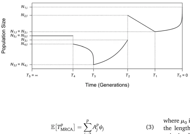
Figure 1 Illustration of an example of a generalized de-mographic model as introduced in the first section of

Materials and Methods. This model consists of five epochs (starting from the present on the right): (1) faster-than-exponential (b.1) growth (forward in time) fromN1;ftoN1;ibetweenT0¼0 andT1;(2) linear

de-cline (a special case of generalized dede-cline whenb¼0) from N2;f to N2;i between T1 and T2; (3) exponential

growth (a special case of generalized growth when

b¼1) fromN3;f toN3;ibetweenT2andT3;(4)

slower-than-exponential (b,1) decline from N4;f to N4;i

be-tween T3 and T4; and (5) constant population size (a

special case of generalized growth when r¼0) at

N5;i¼N5;fstarting fromT4;which lasts indefinitely

back-ward in time (T5¼N). The ending population size of the

previous epoch is not necessarily the beginning popula-tion size of the next epoch (e.g.,N2;f6¼N3;i;N4;f6¼N5;i),

corresponding to an instantaneous population size change at that time.

fk_j ¼ 1 _j 2 2 6 6 6 6 4e 2 j 2

LðTkÞ

Nk;f log Nk;f2e

2

j

2

LðTk21Þ

Nk;i log Nk;i

3 7 7 7 7 5;

rkþ

_j

2

¼0

1

r_kþ

_j 2 2 6 6 6 6 4e 2 j 2

LðTk21Þ

Nk;i2e

2

j

2

LðTkÞ

Nk;f

3 7 7 7 7 5;

rkþ

_j

2

6¼0:

8 > > > > > > > > > > > > > > > > > > > > > > > > > > > > > > > > > > < > > > > > > > > > > > > > > > > > > > > > > > > > > > > > > > > > > : (9)

2. Ifbk.0;rk.0 orbk¼1;rk,0;

fk_j ¼ 1

_j 2 2 6 6 6 6 6 4Nk;iU

0 B B B

@22

1

bk; _j

2

bkrk N2bk

k;i

1 C C C Ae 2 _j 2

LðTk21Þ

2Nk;fU

0 B B B

@22

1

bk; _j

2

bkrk N2bk

k;f

1 C C C Ae 2 _j 2

LðTkÞ 3 7 7 7 7 7 5: (10)

3. Ifbk,0;rk.0;

fk_j ¼1

j 2 2 6 6 6 6 4Nk;fM

0 B B B

@22

1

bk;

j 2

bkrk N2bk

k;f

1 C C C Ae 2 j 2

LðTkÞ

2Nk;iM

0 B B B

@22

1 bk ; j 2

bkrk N2bk

k;i

1 C C C Ae 2 j 2

LðTk21Þ 3 7 7 7 7 5: (11)

The expressions of function LðTÞ are given in File S1. The function Uðb;xÞ:¼xUð1;b;xÞ ¼xR₀Ne2xt_ð1þtÞb22

dt;

whereUða;b;xÞis the confluent hypergeometric function of the second kind (Gradshte˘ın et al. 2007). The function

Mðb;xÞ:¼ ðx=ðb21ÞÞMð1;b;xÞ ¼xR₀1ext_ð12tÞb22

 dt;where

Mða;b;xÞ is the confluent hypergeometric function of the

first kind (Gradshte˘ın et al.2007). The exponential growth or decline then becomes a special case of Uðb;xÞ when

b¼1;x6¼0;

Uð1;xÞ ¼xex

Z _N

1 e2t

t dt¼xe x_E

1ðxÞ; (12)

where E1ðxÞ is the exponential integral (Gradshte˘ın et al.

2007), which has been shown by previous studies (Polanski

et al.2003; Bhaskaret al.2015). We could notfind feasible and numerically stable closed-form formulas forfk_jwhen the population size decreases forward in time in a manner that is not linear or exponential (i.e.,rk,0 andbkÏf0;1g). In these

scenarios, we used Gauss–Legendre quadrature (Kahaner

et al. 1988) for efficient numerical evaluation of relevant functions (seeFile S1for detailed description).

Software implementation

The above expressions are implemented in a software pack-age, EGGS. The source code and compiled programs for Linux and Mac OS platforms are publicly available from our Web site (http://keinanlab.cb.bscb.cornell.edu). Source code was written in C++, with no external libraries needed for com-pilation. Additional information of implementation is in-cluded in File S1 and in the manual that accompanies the software online.

Demographic models assumed in this study

The demographic models used in this study are based on the inferred European history presented by Gazave et al.

(2014) (Figure 2, in black), which contains two bottlenecks (Keinanet al.2007) and a recent exponential growth ep-och. Specifically, the Gazaveet al. (2014) model inferred that the European population had a constant effective pop-ulation size of 10,000 (diploid) individuals before 4720 generations ago and went through the ancient bottleneck between 4720 and 4620 generations ago with a population size of 189. The population size then recovered to 10,000 diploids until 720 generations ago, at which time the recent bottleneck started with a size of 549. At 620 generations ago, the population size recovered to 5633 individuals. The recent growth epoch started 140.8 generations ago and led to a population size of 654,000 at present. The param-eters of the original recent growth epoch were varied to incorporate generalized growth effects.

In addition to using the model mentioned above, we also applied an alternative model of ancient European history for inference. The model was first presented in Gravel et al.

(2011) and later used in Tennessenet al.(2012). This model inferred that the European population had an ancient effec-tive population size of 7300 diploid individuals until 6167 generations ago, when the population size expanded to 14,474 individuals. Thefirst bottleneck took place 2125 gen-erations ago, with the population size reducing to 1861 indi-viduals. Thisfirst bottleneck lasted until 958 generations ago, at which time a second bottleneck took place with a

decreased population size of 1032. We assumed 24 years per generation (Scally and Durbin 2012) to translate the year-based time presented in the original model. For compatibility with the Gazaveet al.(2014) model, we considered that the population size had an instantaneous recovery after the sec-ond bottleneck lasted for 100 generations, instead of gradual recovery (Gazaveet al.2014).Figure S8shows the schematic representation of the Gravelet al.(2011) model.

Demographic inference framework based on the site frequency spectrum

Demographic inference in this study was based on the ob-served allele frequency counts from the simulated or real data set. To determine thefitness of a modelNðTÞto the observed data, we calculated the composite log likelihood by

L½N ¼log E½jjN ¼CE½jjN; (13)

whereCis a vector of the observed folded allele frequency counts andE½jjNis the computed folded SFS under demo-graphic modelNðTÞ:More detailed description can be found inFile S1.

To search for the maximum-likelihood point over the parameter space, we applied the ECM (Expectation/ Conditional Maximization) method (Meng and Rubin 1993), which was previously used in the demographic inference study by Excoffier et al. (2013). One hundred ECM cycles were

performed for each run of inference. We obtained 95% confi -dence intervals of parameter estimates via block bootstrapping of the data 200 times. Specifically, if the original data containedl

loci, we randomly choselloci from the original data with re-placement in each bootstrap (seeFile S1for details).

Processing of NHLBI Exome Sequencing Project data for demographic history inference

The NHLBI Exome Sequencing Project (ESP) data (Tennessen

et al.2012; Fuet al.2013) contain deep sequencing of 4300 individuals of European ancestry. An important feature of these data is the high level of sequencing coverage, which allows the capture of very rare variants accurately. These variants constitute the part of the SFS that is most enriched for information on recent population growth (Keinan and Clark 2012; Tennessenet al.2012; Gao and Keinan 2014). To reduce the effect of selection as much as possible while keeping a sufficient amount of data, we chose to use the SFS calculated from synonymous single-nucleotide variants (SNVs) only, as previously performed by Tennessen et al.

(2012). To further improve the quality of the data, wefiltered SNVs with average read depth#20 or with successful geno-type counts ,7740 (90%) and subsampled the remaining 233,134 SNVs to 7740 alleles, which is equivalent to 3870 diploid individuals (File S1).

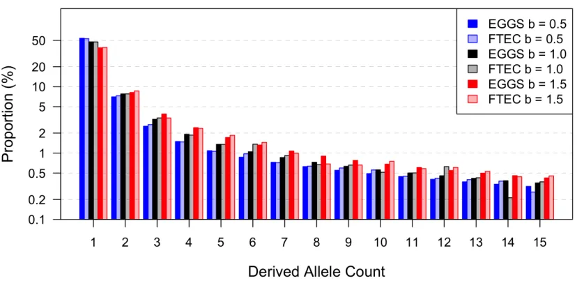
Figure 2 Comparison of four summary statistics estimated by FTEC simulation and computed by EGGS. (A) Demonstration of the demographic models considered for evaluating the accuracy of our calculations as implemented in EGGS (first sec-tion ofResults). This two-bottleneck model has the same population size and time throughout history as in the inferred European history in Gazaveet al.

(2014), with the exception that we varied the growth speed parameter of the recent growth ep-och to beb¼0:5 (sub-exponential, blue),b¼1:0 (exponential as in Gazaveet al.2014, black), and

b¼1:5 (super-exponential, red). They-axis shows effective population size of diploid individuals on log scale. (B–E) The comparison of thefirst 15 en-tries of the SFS (B), the total number of segregating sites (S) across all 200,000 loci (each 1000 bp long) (C), the expected pairwise difference between chromosomes per base pair (D), and the burden of private mutations (a) as the percentage of het-erozygous variants in one individual that are mono-morphic in the rest of the sample of 999 individuals (E) computed numerically in EGGS (dark-colored bars) and simulated by FTEC (light-colored bars) for the demographic models shown in A: blue,

b¼0:5;black,b¼1:0;red,b¼1:5;with a sam-ple size of 1000 individuals (2000 chromosomes). They-axis in B is on a log scale.

Data availability

The NHLBI Exome Sequencing Project (ESP) data used in this study is publicly available at http://evs.gs.washington. edu/EVS/.

Results

Comparison with simulated results by FTEC

To validate that the expressions provided in Materials and Methodscan correctly compute the summary statistics under generalized growth models, we compared the summary sta-tistics calculated by our software EGGS to those simulated by the software FTEC (a coalescent simulator for modeling faster than exponential growth by Reppellet al.2012) under the demographic models shown in Figure 2A. This model is the inferred European history in Gazaveet al.(2014), except that we varied the growth speed parameterb(Equation 1), which corresponds to 1 in the original model (exponen-tial growth), to also be 0.5 (corresponding to sub-exponen(exponen-tial growth) and 1.5 (corresponding to super-exponential growth). The sample size isfixed at 1000 diploid individuals (2000 chromosomes). For FTEC simulation, we used a mu-tation rate of 1:231028_{per base pair per generation (e.g.,}

Kong et al.2012) and simulated 200,000 independent loci, each of 1000 bp.

The comparison of the SFS,S(across all 200,000 loci),p, andanumerically computed by EGGS to those simulated by FTEC is shown in Figure 2, B–E. For each demographic model illustrated in Figure 2A, the values for all summary statistics from the numerical computation by EGGS are practically identical to those from the simulation results by FTEC. How-ever, our software EGGS exhibits a huge speed improvement over FTEC. For each model considered in Figure 2A, EGGS takes,1 sec to generate the results, while it takes5 hr for FTEC to simulate the sequences, due to the large number of independent loci required for accurate estimation (per-formed in the Ubuntu system with an Intel Xeon CPU at 2.67 GHz). For instance, when 2000 independent loci are simulated, which still takes3 min, the summary statistics deviate considerably from the accurate results (Figure S2and

Table S1). Furthermore, our software works well over a wide range of values of the growth parameterb, even whenb¼0 (corresponding to linear growth or decline) orb,0 (Figure S3), conditions that are not handled by FTEC. We note, how-ever, that as a simulation program FTEC provides the full sequences as output and can have a wider range of applica-tions than facilitated by the SFS and other summary statistics that EGGS calculates.

Evaluating inference of generalized growth based on the site frequency spectrum

We next set out to test the accuracy (as a function of sample size) of inferring parameters in models with generalized growth from the SFS. Bhaskar and Song (2014) showed that in theory, an underlying generalized growth demographic

model can be uniquely identified by the ideal, perfect expected SFS with a very small sample size generated from that model (34 haploid sequences for the models shown in Figure 2A). However, the SFS is estimated in practice from a limited amount of data from each individual (even in the case of whole-genome sequencing) and, as a result, the estimated SFS will fluctuate around the expected values, which limits its accuracy for inference (Terhorst and Song 2015). We aim to test such inference in practice and determine the power of generalized growth detection and the sample size needed for accurately recovering the growth speed parameter as well as other parameters of the demographic model. For it to be comparable with many practical applications, we considered sequence length that is about equivalent to that obtained from whole-exome sequencing (File S1).

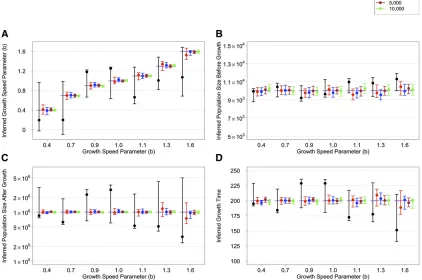
We performed inference on the SFS calculated from sim-ulated sequences generated by FTEC. We simsim-ulated a de-mographic model with the same initial epochs as the model illustrated in Figure 2A. Starting 620 generations ago, the simulated model includes a constant population size of 10,000 until 200 generations ago, when the population starts a generalized growth epoch until the present. The general-ized growth epoch starts with a population size of 10,000 that grows to an extant effective population size of 1 million in-dividuals, with the growth speed parameterbtaking each of the following values: 0.4, 0.7, 0.9, 1.0, 1.1, 1.3, and 1.6. We chose these values to represent a range of super-exponential and sub-exponential growth, with emphasis on values around the exponential rate (b¼1:0) to test the detection power of generalized growth when the growth speed devi-ates slightly from exponential. We varied the sample size (number of diploid individuals sampled at present) to be 1000, 2000, 3000, 5000, and 10,000 (File S1). Thefirst 15 entries of the site frequency spectra for these simulated sce-narios are shown inFigure S4. From each set of simulations, we then inferred four parameters of the recent growth epoch, which can uniquely determine the epoch: (1) the growth speed parameter b; (2) the initial population size before growth,Nf;(3) the ending population size after growth,Ni;

and (4) the onset time of growthT, which is equivalent to the growth duration since the simulated epoch ends at present.

As sample size increases, the accuracy of the point esti-mates generally improves and the confidence interval narrows (Figure 3). Specifically, when the SFS of only 1000 diploids is used for inference, the inference performs poorly for all pa-rameters, exhibiting large confidence intervals (Figure 3). However, the confidence interval always includes the true simulated value. A sample size of 2000 already exhibits acceptable performance except when the growth speed becomes large (b¼1:3 and 1.6). Larger sample sizes of 5000 and 10,000 are sufficient for inferring all parameters with very tight confidence intervals. For such sample sizes, the inference even significantly distinguishes between growth speeds (b¼0:9 andb¼1:1) that are close to expo-nential (b¼1:0) from that of an exponential, thereby con-cluding that a sub-exponential (0.9) or super-exponential

(1.1) growth has taken place. These observations suggest that a sample size of at least 3000 diploid individuals might be needed for inferring the parameters associated with the simulated recent generalized growth epoch, which is moti-vated by previous models of European demographic history. It remains to be explored how accurate the estimates are, and how their accuracy improves with sample size, across a more diverse set of models.

European demographic history inference

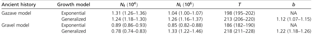
We next performed demographic inference on NHLBI ESP data (Tennessenet al.2012; Fuet al.2013). We applied our inference framework to these data while considering and comparing two models. Both models assume the ancient epochs before 620 generations ago to be the same as those in the Gazaveet al.(2014) model illustrated in Figure 2A. We inferred the parameters only for the most recent epoch, which is of generalizedgrowth in one model while limited toexponentialgrowth in the other. The parameters for infer-ence are as follows: for both models, (1) population size before growth (Nf); (2) population size after growth (Ni);

and (3) growth onset time (T), which is equivalent to the

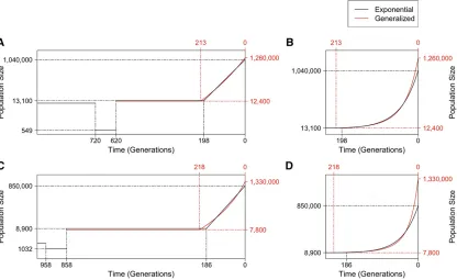
duration of growth; and only for the generalized growth model (4) the growth speed parameter (b), which isfixed atb¼1 for the exponential growth model. The point esti-mates and 95% confidence intervals are shown in Table 1 and the best-fit demographic models are illustrated in Figure 4, A and B (see alsoFigure S5,Figure S6andFigure S7).

Although the Gazaveet al.(2014) model assumed a dif-ferent ancient history before the recent growth epoch from that assumed in Tennessenet al.(2012), using ESP data and assuming exponential growth, the inferred growth epoch is generally consistent with that obtained in the latter study (Figure 4, A and B, and Table 1). Our study infers that recent growth started 198 (95% C.I.: 195–202) generations ago with an effective population size of 13,100 (12,600– 13,600) and continued at a rate of 2.2% (2.15–2.26%) per generation (Table 1), while Tennessen et al. (2012) esti-mated that recent growth had an initial population size of

9500 individuals, a duration of 204 generations, and a growth rate of 2.0% per generation.

Theinferred generalizedgrowthmodelfitsthedatasignificantly better than that with exponential growth (P-value¼3:8531026

by x2 _{likelihood-ratio test with 1 d.f.). It estimates that}

Figure 3 Inference results on simulated data with a recent generalized growth epoch. The model parameters are as follows: Growth starts 200 generations before the present from an effective population size of 10,000 and ends with an effective population size of 1 million at present. The growth speed parameterbtakes the following values in different simulations: 0.4, 0.7, 0.9, 1.0, 1.1, 1.3, and 1.6. Inference of these four parameters is based on the SFS estimated from a sample of individuals of one offive sizes (black, 1000; red, 2000; blue, 3000; brown, 5000; and green, 10,000). The point estimates with 95% confidence interval for these parameters are grouped by the growth speed parameterb(x-axis). The thick, dashed lines show the true values of the simulated model. The results are shown in the following order: (A) the inferred growth speed parameter, (B) the inferred population size before growth, (C) the inferred population size after growth, and (D) the inferred growth start time. They-axis in C is on a log scale.

growth started 213 (206–220) generations ago from an ef-fective population size of 12,400 (11,800–13,000), both values consistent with those estimated in the exponential growth model. The extant effective population size following growth is estimated to be 1.26 (1.16–1.37) million. The inferred growth speed parameter b¼1:12 (1.07–1.15) is significantly larger than the exponential speed of b¼1 (P-value10212_{;using a one-tailedz-test), which is the main}

difference between the two models.b¼1:12 implies a growth rate acceleration pattern (File S1) that is super-exponential at 12% faster than exponential through the epoch (Figure 4): the super-exponential growth is relatively slow around the onset time, and it keeps accelerating as time approaches the present.

To test the sensitivity of the model to the assumption of ancient European history, we considered an alternate model of ancient history. Wefixed the history before 858 generation ago to be that inferred by Gravel et al. (2011) for Europeans (Materials and Methods). We repeated inference of the same parameters, using the same ESP data. As above, the inferred parameters for exponential growth are similar to those obtained in Tennessenet al.(2012) that were based on the model of Gravelet al.(2011) (Table 1). However, the SFS from this modelfits the data worse than that from the expo-nential model based on the ancient history of the Gazaveet al.

(2014) model (P-value¼1:5931026 _fromx2

goodness-of-fit test between the exponential Gravel model and ESP data;

P-value ¼ 0.97 for the corresponding exponential Gazave model; seeFile S1andTable S3). By applying a generalized growth epoch to the Gravelet al.(2011) model, the inferred parameters are generally in line with those from the gener-alized model based on Gazaveet al.(2014), although some differences exist (Table 1), indicating that the assumption of ancient history can affect the inference of recent growth to some extent. More importantly, the generalized Gravel model

fits the data almost equally well as the generalized Gazave model, which is significantly better than the exponential model (P-value 10212 _{by x}2 _{likelihood-ratio test; also}

see Table S3). As with the generalized Gazave model, the inferred growth speed parameter from the generalized Gravel model, b¼1:22 (1.18–1.26), is also significantly larger than the exponential speed b¼1 (P-value10212_;

using a one-tailedz-test; Figure 4, C and D).

Motivated by these results, we considered a third model with two recent exponential growth epochs, which still

assumes the ancient epochs before 620 generations ago to be the same as those in the Gazaveet al.(2014) model illus-trated in Figure 2A. Five parameters were inferred (Table S2), with the first phase of growth estimated to start 219 (95–334) generations ago with a population size of 12,200 (11,700–13,200). This phase of growth lasts until 135 (25– 157) generations ago and leads to a population size of 47,100 (30,200–540,900). The population size after the recent phase of growth is 1.12 (1.07–2.09) million. This model provides a significantly betterfit than the model with a single exponential growth (P-value¼5:5531026_byx2

likelihood-ratio test with 2 d.f.), but is a worse model than the general-ized growth model (based on the Bayesian information criterion, BICtwo-epoch exponential2BICgeneralized¼6:1).

How-ever, this model exhibits some of the same accelerating pat-terns as in the generalized growth model, ascertained by the growth rate of the most recent exponential epoch being 2.4% (2.3–5.2%), larger than that of thefirst exponential epoch, 1.6% (1.3–2.1%). This acceleration pattern shown in both the generalized model and the model with two exponential epochs is consistent with evidence of growth in European census population size that has greatly accelerated in the modern era (Keinan and Clark 2012).

Discussion

In this study, we provide mathematical derivation and a software that can efficiently compute the expected values of five genetic data summary statistics given a generalized demographic model by evaluating the derived explicit expres-sions. These summary statistics include the time to the most recent common ancestor (TMRCA), the total number of

segre-gating sites (S), the SFS, the average pairwise difference be-tween chromosomes per site (p), and the burden of private mutations (a). The fast and accurate generation of these summary statistics under generalized models can provide a useful tool in the studies of human demographic inference. For instance, in addition to inference based on the SFS as in the present study, a recent study by Chenet al.(2015) pre-sented an inference framework based on the total number of segregating sites. The results in this study can be easily in-corporated into that framework. Furthermore, the source code of the software is freely available to allow extensions to compute other summary statistics of interest (for example, the joint SFS of samples from multiple populations under

Table 1 Demographic inference results using ESP data for a model with a recent epoch of exponential growth and a model with a recent epoch of generalized growth

Ancient history Growth model Nf ð104Þ Ni ð106Þ T b

Gazave model Exponential 1.31 (1.26–1.36) 1.04 (1.00–1.07) 198 (195–202) NA

Generalized 1.24 (1.18–1.30) 1.26 (1.16–1.37) 213 (206–220) 1.12 (1.07–1.15)

Gravel model Exponential 0.89 (0.86–0.93) 0.85 (0.82–0.88) 186 (182–190) NA

Generalized 0.78 (0.74–0.83) 1.33 (1.22–1.46) 218 (211–228) 1.22 (1.18–1.26)

Shown are point estimates and 95% confident intervals (in parentheses) for the following parameters of the inferred recent growth epoch when the ancient history was assumed to be the same as that in the Gazaveet al.(2014) model and the Gravelet al.(2011) model: population size before growth (Nf); population size after growth (Ni);

time growth started in generations (T); and the growth speed parameter (b), which isfixed atb¼1 in the exponential growth case.

generalized models, by extending the work of Wakeley and Hey 1997 and Chen 2012). Such extensions can facilitate a variety of population genetic studies in humans and other organisms beyond the inference of demographic history.

It is also possible that other families of growth models may

fit the pattern of human population size history. For instance, Eldonet al.(2015) considered the algebraic-growth model in the form of NðTÞ ¼Tg_{: In reality, however, not all}

demo-graphic models have numerically stable closed-form expres-sions for the expected time to thefirst coalescent event (cj).

In these cases, fast and accurate numerical integration meth-ods, such as the Gauss–Legendre quadrature used in this work, can be applied to evaluate cj:This technique holds

the promise of efficiently generating the expected value of population genetic summary statistics under arbitrary popu-lation size functions.

Bhaskaret al.(2014) pointed out that as sample size in-creases, the assumptions of standard Kingman’s coalescent are violated as multi-merger and simultaneous-merger events can become nonnegligible. Such events can distort the genealogies and potentially cause the values of summary statistics to be different from those under Kingman’s coales-cent (Bhaskar et al. 2014). To explore such discrepancies, we compared the SFS from Kingman’s coalescent and the discrete-time Wright–Fisher (DTWF) model (Bhaskaret al.

2014) under the inferred demographic history in the gener-alized Gazave model with a sample size of 3870 diploids (File S1). We observed that the SFS from the DTWF model and Kingman’s coalescent are very similar (File S1 and Figure S9), which means that multi-merger and simultaneous-merger events should not have a significant effect on the inference carried out in this study. However, it remains valu-able to systematically study the effect of multi-merger and simultaneous-merger events in the context of generalized growth, especially as sample size increases.

By applying inference of generalized growth based on the SFS generated from the synonymous variants of 4300 indi-viduals of the NHLBI ESP data set (Tennessenet al.2012; Fu

et al. 2013), we found that the generalized growth model shows a betterfit to the observed data than the exponential growth model that has been used by almost all previous de-mographic modeling studies (P-value ¼3:8531026_{). We}

also found that the European population experienced a re-cent growth in population size with speed modestly faster than exponential (b¼1:12;P-value10212_{for difference}

fromb¼1). This result is consistent with previous specula-tions that the human population might have undergone a recent accelerated growth epoch based on the observation of very rare, previously unknown variants in several sequenc-ing studies with large sample sizes (Nelson et al. 2012;

Figure 4 Demographic inference results based on ESP data. (A) Illustration of the effective population size (y-axis, on a log scale) over time for the best-fit models inferred based on ESP data, assuming the ancient history is the same as that in Gazaveet al.(2014). Two models are shown: one restricted to recent growth being exponential (black) and one with a generalized recent growth epoch (red). Before 620 generations ago, the model was not inferred and all parameters were set to be the same as those shown in Figure 2A. Solid lines show the effective population size over time for each of the inferred models, with dashed lines indicating estimated parameter values on thex-axis or they-axis. Only the most recent 1000 generations are shown to emphasize the difference between the two models. (B) A zoom-in to the most recent 240 generations of the inferred models in A to emphasize the acceleration pattern of the generalized growth model, with they-axis on a linear scale. (C-D) Similar to A-B, except that the best-fit models presented are based on the assumption that the ancient history before 858 generations ago isfixed to that in Gravelet al.(2011) (seeFigure S8).

Tennessenet al.2012; Fuet al.2013). It is also in line with the super-exponential growth in census population size dur-ing that time (Keinan and Clark 2012). In future studies, it will be valuable to incorporate gradient-based optimization techniques for the fast inference of demographic models con-taining generalized growth epochs, e.g., by extending the work of Bhaskar et al. (2015). Such an improvement will enable simultaneous inference of recent growth and more ancient epochs.

To minimize the impact of natural selection on our de-mographic inference, we considered only synonymous SNVs for demographic modeling, as in the original study of Tennessenet al.(2012). However, it is still a potential limita-tion that the data are affected by negative and background selection. Hence, it remains valuable to validate the result of super-exponential growth by conducting inference on SFS calculated from more neutral genomic regions (Gazave

et al. 2014) or by modeling the effect of selection. One promising possibility is extracting genomic regions that are less subject to selection from whole-genome sequences in the UK10K project (The UK10K Consortiumet al.2015). More generally, with the increasing availability of high-quality whole-genome sequencing data with large sample sizes for humans and other species, more refined and re-alistic demographic histories can be estimated with gener-alized models.

Acknowledgments

The authors thank Leonardo Arbiza for helpful comments; Yun S. Song, Andrew G. Clark, and two anonymous reviewers for insightful comments on earlier versions of this manuscript; and Arjun Biddanda for his careful editing of the software manual. This work was supported by National Institutes of Health grants R01GM108805 and R01HG006849, an award from The Ellison Medical Foun-dation, and an award from The Edward Mallinckrodt, Jr. Foundation. Feng Gao is a Howard Hughes Medical Institute International Student Research fellow.

Literature Cited

Arbiza, L., S. Gottipati, A. Siepel, and A. Keinan, 2014 Contrasting X-linked and autosomal diversity across 14 human populations. Am. J. Hum. Genet. 94(6): 827–844.

Bhaskar, A., and Y. S. Song, 2014 Descartes’rule of signs and the identifiability of population demographic models from genomic variation data. Ann. Stat. 42(6): 2469–2493.

Bhaskar, A., A. G. Clark, and Y. S. Song, 2014 Distortion of gene-alogical properties when the sample is very large. Proc. Natl. Acad. Sci. USA 111(6): 2385–2390.

Bhaskar, A., Y. X. Wang, and Y. S. Song, 2015 Efficient inference of population size histories and locus-specific mutation rates from large-sample genomic variation data. Genome Res. 25(2): 268–279.

Chen, H., 2012 The joint allele frequency spectrum of multiple populations: a coalescent theory approach. Theor. Popul. Biol. 81(2): 179_–195.

Chen, H., J. Hey, and K. Chen, 2015 Inferring very recent popu-lation growth rate from popupopu-lation-scale sequencing data: using a large-sample coalescent estimator. Mol. Biol. Evol. 32(11): 2996–3011.

Coventry, A., L. M. Bull-Otterson, X. Liu, A. G. Clark, T. J. Maxwell et al., 2010 Deep resequencing reveals excess rare recent var-iants consistent with explosive population growth. Nat. Com-mun. 1: 131.

Eldon, B., M. Birkner, J. Blath, and F. Freund, 2015 Can the site-frequency spectrum distinguish exponential population growth from multiple-merger coalescents? Genetics 199: 841–856. Excoffier, L., I. Dupanloup, E. Huerta-Sanchez, V. C. Sousa, and M.

Foll, 2013 Robust demographic inference from genomic and SNP data. PLoS Genet. 9(10): e1003905.

Fu, W., T. D. O_’Connor, G. Jun, H. M. Kang, G. Abecasiset al., 2013 Analysis of 6,515 exomes reveals the recent origin of most human protein-coding variants. Nature 493(7431): 216_–220.

Gao, F., and A. Keinan, 2014 High burden of private mutations due to explosive human population growth and purifying selec-tion. BMC Genomics 15(Suppl. 4): S3.

Gazave, E., L. Ma, D. Chang, A. Coventry, F. Gao et al., 2014 Neutral genomic regions refine models of recent rapid human population growth. Proc. Natl. Acad. Sci. USA 111(2): 757–762.

Gottipati, S., L. Arbiza, A. Siepel, A. G. Clark, and A. Keinan, 2011 Analyses of X-linked and autosomal genetic variation in population-scale whole genome sequencing. Nat. Genet. 43(8): 741–743.

Gradshte˘ın, I. S., I. M. Ryzhik, and A. Jeffrey, 2007 Table of Inte-grals,Series,and Products, Ed. 7. Academic Press, Amsterdam/ Boston.

Gravel, S., B. M. Henn, R. N. Gutenkunst, A. R. Indap, G. T. Marth et al., 2011 Demographic history and rare allele sharing among human populations. Proc. Natl. Acad. Sci. USA 108(29): 11983–11988.

Gutenkunst, R. N., R. D. Hernandez, S. H. Williamson, and C. D. Bustamante, 2009 Inferring the joint demographic history of multiple populations from multidimensional SNP frequency data. PLoS Genet. 5(10): e1000695.

Hammer, M. F., F. L. Mendez, M. P. Cox, A. E. Woerner, and J. D. Wall, 2008 Sex-biased evolutionary forces shape genomic patterns of human diversity. PLoS Genet. 4(9): e1000202.

Harris, K., and R. Nielsen, 2013 Inferring demographic history from a spectrum of shared haplotype lengths. PLoS Genet. 9(6): e1003521.

Hudson, R. R., 2002 Generating samples under a Wright-Fisher neutral model of genetic variation. Bioinformatics 18(2): 337–338.

Kahaner, D., C. B. Moler, S. Nash, and G. E. Forsythe, 1988 Numerical Methods and Software. Prentice Hall, Engle-wood Cliffs, NJ.

Keinan, A., and A. G. Clark, 2012 Recent explosive human pop-ulation growth has resulted in an excess of rare genetic variants. Science 336(6082): 740–743.

Keinan, A., J. C. Mullikin, N. Patterson, and D. Reich, 2007 Measurement of the human allele frequency spectrum demonstrates greater genetic drift in East Asians than in Euro-peans. Nat. Genet. 39(10): 1251–1255.

Keinan, A., J. C. Mullikin, N. Patterson, and D. Reich, 2009 Accelerated genetic drift on chromosome X during the human dispersal out of Africa. Nat. Genet. 41(1): 66–70. Kingman, K. F. C., 1982a On the genealogy of large populations.

J. Appl. Probab. 19: 27_–43.

Kingman, K. F. C., 1982b The coalescent. Stoch. Proc. Appl. 13(3): 235_–248.

Kong, A., M. L. Frigge, G. Masson, S. Besenbacher, P. Sulemet al., 2012 Rate of de novo mutations and the importance of father’s age to disease risk. Nature 488(7412): 471–475.

Li, H., and R. Durbin, 2011 Inference of human population history from individual whole-genome sequences. Nature 475(7357): 493–496.

Liu, X., and Y. X. Fu, 2015 Exploring population size changes using SNP frequency spectra. Nat. Genet. 47(5): 555–559. MacLeod, I. M., D. M. Larkin, H. A. Lewin, B. J. Hayes, and M. E.

Goddard, 2013 Inferring demography from runs of homozy-gosity in whole-genome sequence, with correction for sequence errors. Mol. Biol. Evol. 30(9): 2209_–2223.

Marth, G. T., E. Czabarka, J. Murvai, and S. T. Sherry, 2004 The allele frequency spectrum in genome-wide human variation data reveals signals of differential demographic history in three large world populations. Genetics 166: 351–372.

Meng, X. L., and D. B. Rubin, 1993 Maximum-likelihood-estimation via the Ecm algorithm - a general framework. Biometrika 80(2): 267–278.

Nelson, M. R., D. Wegmann, M. G. Ehm, D. Kessner, P. St Jean et al., 2012 An abundance of rare functional variants in 202 drug target genes sequenced in 14,002 people. Science 337(6090): 100–104.

Polanski, A., and M. Kimmel, 2003 New explicit expressions for relative frequencies of single-nucleotide polymorphisms with application to statistical inference on population growth. Genet-ics 165: 427–436.

Polanski, A., A. Bobrowski, and M. Kimmel, 2003 A note on dis-tributions of times to coalescence, under time-dependent pop-ulation size. Theor. Popul. Biol. 63(1): 33_–40.

Reppell, M., M. Boehnke, and S. Zollner, 2012 FTEC: a coalescent simulator for modeling faster than exponential growth. Bioin-formatics 28(9): 1282–1283.

Reppell, M., M. Boehnke, and S. Zollner, 2014 The impact of accelerating faster than exponential population growth on ge-netic variation. Gege-netics 196: 819–828.

Scally, A., and R. Durbin, 2012 Revising the human mutation rate: implications for understanding human evolution. Nat. Rev. Genet. 13(10): 745–753.

Schiffels, S., and R. Durbin, 2014 Inferring human population size and separation history from multiple genome sequences. Nat. Genet. 46(8): 919–925.

Sheehan, S., K. Harris, and Y. S. Song, 2013 Estimating variable effective population sizes from multiple genomes: a sequentially Markov conditional sampling distribution approach. Genetics 194: 647–662.

Takahata, N., and M. Nei, 1985 Gene genealogy and variance of interpopulational nucleotide differences. Genetics 110: 325–344. Tavare, S., 1984 Line-of-descent and genealogical processes, and their applications in population-genetics models. Theor. Popul. Biol. 26(2): 119–164.

Tennessen, J. A., A. W. Bigham, T. D. O’Connor, W. Fu, E. E. Kenny et al., 2012 Evolution and functional impact of rare coding variation from deep sequencing of human exomes. Science 337(6090): 64–69.

The UK10K Consortium, K. Walter, J. L. Min, J. Huang, L. Crooks et al., 2015 The UK10K project identifies rare variants in health and disease. Nature 526(7571): 82–90.

Terhorst, J., and Y. S. Song, 2015 Fundamental limits on the accuracy of demographic inference based on the sample fre-quency spectrum. Proc. Natl. Acad. Sci. USA 112(25): 7677– 7682.

Wakeley, J., and J. Hey, 1997 Estimating ancestral population parameters. Genetics 145: 847–855.

Communicating editor: S. Ramachandran

GENETICS

Supporting Information

www.genetics.org/lookup/suppl/doi:10.1534/genetics.115.180570/-/DC1

Inference of Super-exponential Human Population Growth

via Ef

fi

cient Computation of the Site Frequency Spectrum for

Generalized Models

Feng Gao and Alon Keinan

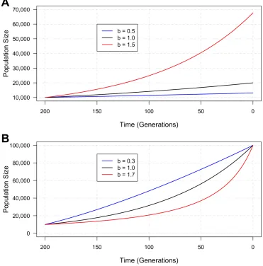
Figure S1. Different patterns of generalized growth.

(A) Illustration of the population size

functions when keeping the population size before growth

N

f

, the growth time

T

and the parameter

r

the same and varying the growth speed parameter

b

to be 0.5, 1.0 and 1.5. (B) Illustration of the

population size functions when keeping the population size before growth

N

f

, the population size

after growth

Ni

and the growth time

T

the same and varying the growth speed parameter

b

to be

Figure S2. Comparison of the first 15 entries of the SFS computed numerically in

EGGS

(dark bars) and simulated result by

FTEC

(light bars)

. Only 2,000 loci (1,000 bp-long each)

instead of 200,000 were simulated for the demographic models shown in Figure 2(A):

b

= 0

.

5, blue;

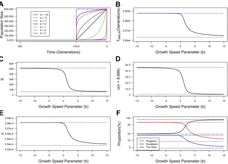
Figure S3. Expected values of summary statistics generated under demographic

mod-els with a wide range of the growth speed parameter (

b

)

. The time values and population

size values are kept the same as shown in Figure 2(A). The growth speed parameter (

b

) of the recent

epoch takes values from

−

15 to 15. The sample size is 10,000 individuals. The mutation rate per

site per generation

µ0

= 1

.

2

×

10

−8

. We assumed a total of 2

×

10

8

sites , thus the locus-based

mutation rate

µ

= 2

.

4 (same for Figure 2). (A) The demonstration of the demographic models for

several values of

b

. To better exhibit the difference between different values of

b

, only the most

recent 400 generations are shown. The two dotted purple lines show the constant-size model fixed

at 5,633 (corresponding to

b

→ ∞

) and an instant-increase model with a sudden change from 5,633

to 654,000 at 140.8 generations ago (corresponding to

b

→ −∞

). (B)-(E) The expected value of

T

MRCA

,

S

,

α

at

n

= 9,999 and

π

respectively for

b

varying from

−

15 to 15. The two dotted purple

lines correspond to the expected values for the scenarios shown by the dotted purple lines in (A).

(F) The expected proportion of singletons (red), doubletons (blue) and the sum of the rest entries

of the SFS for

b

varying from

−

15 to 15. The dotted lines show expected singletons (red),

Figure S4. The first 15 entries of the site frequency spectra for the simulation

sce-narios described in the second section of Results.

The inference results are shown in Figure

3. (A)-(G): corresponding to

b

= 0

.

4,

b

= 0

.

7,

b

= 0

.

9,

b

= 1

.

0,

b

= 1

.

1,

b

= 1

.

3 and

b

= 1

.

6

re-spectively for the recent generalized growth epoch, with sample size of 1,000 diploids (blue), 2,000

Figure S5. The one-dimensional log likelihood surface around the best estimates of the

ESP synonymous data using exponential growth model

. (A) varying population size before

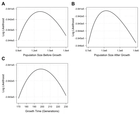
growth while keeping all other parameters at corresponding best estimates; (B) varying population

Figure S6. The one-dimensional log likelihood surface around the best estimates of the

ESP synonymous data using generalized growth model.

(A) varying population size before

growth while keeping all other parameters at corresponding best estimates; (B) varying

Figure S7. The first 20 entries of the site frequency spectra for ESP data and the

in-ferred demographic models assuming the ancient demography in Gazave

et al.

(2014).

The SFS from the ESP data, the exponential model, the generalized growth model and the

two-epoch exponential model are shown in black, green, red and blue respectively. For comparison

purposes, we also included the SFS from a base model, which has a constant population size

Figure S8. The best-fit generalized models for ESP data assuming the ancient

demog-raphy in Gazave

et al.

(2014) (red) and in Gravel

et al.

(2011) (blue).

The demographic

history was fixed before 620 generations ago for Gravel model and 858 generations ago for Gravel

Figure S9. Effects of multi-merger and simultaneous-merger events on the SFS.

The

underlying demographic model is the best-fit generalized model using the ancient history in Gazave

et al

. (2014). The sample size is 3,870 diploid individuals. (A) The 100-entry

partially normalized

SFS under Kingman’s coalescent and under discrete-time Wright-Fisher model. (B) The percentage

difference of entry-to-singleton ratio between Kingman’s coalescent and discrete-time Wright-Fisher

Table S1. Comparison of summary statistics computed by

EGGS

and estimated by

FTEC

simulation.

Only 2,000 loci (1,000 bp-long each) were simulated for the demographic models

shown in Figure 2(A). Presented are (i) the total number of segregating sites (

S

) across all 2,000

loci (1,000 bp-long each), (ii) the mean pairwise difference between chromosomes per base pair

(

π

), and (iii) the burden of private mutation (

α

) as the percentage of heterozygous variants in one

individual that are monomorphic in the rest of the sample of 999 individuals.

Values of

b

0.5

1.0

1.5

S

(10

−4

)

EGGS

10.06

9.70

7.72

FTEC

10.06

8.96

7.73

π

(10

−4

)

EGGS

3.58

3.57

3.57

FTEC

3.53

3.49

3.56

α

(10

−3

)

EGGS

7.56

5.97

4.18

Table S2. Demographic inference results using ESP data for a model with two

re-cent epochs of exponential growth.

Shown are point estimates and 95% confident intervals

(in parenthesis) for the following parameters of the inferred epoch: population size before growth

(

N

2

), population size after the more ancient phase of exponential growth (

N

1

), population size

after the recent phase of exponential growth (

N0

), time when the ancient phase of exponential

growth started (

T

2

, in generations), time when the recent phase of exponential growth started (

T

1

,

in generations).

N

2

(10

4

)

N

1

(10

4

)

N

0

(10

6

)

T

2

T

1

1.22

4.71

1.12

219

135

Table S3. Goodness of fit between the SFS from inferred models and ESP data.

We

show the

p

-value from

χ

2

goodness of fit test and KL divergence between the SFS from the ESP

data and that from the constant population size model, the inferred exponential model, the

gener-alized model and the two-epoch exponential model. The assumed ancient history (Gazave model

or Gravel model) is indicated in parenthesis. The constant population size model is included here

for comparison purposes.

Model

p

-value from

χ

2

test

KL divergence

Constant

0

0.84

Exponential (Gazave)

0.97

1

.

64

×

10

−4

Generalized (Gazave)

1

1

.

15

×

10

−4

Two-Epoch Exponential (Gazave)

1

1

.

09

×

10

−4

Exponential (Gravel)

1

.

59

×

10

−6

4

.

12

×

10

−4

File S1

1

Detailed description of genetic summary statistics

1.1

Total number of segregating sites (

S

)

Suppose we have

n

sequences (chromosomes), this quantity stands for the number of sites in which

the sequences have different genotypes. Namely, if all sequences have a common genotype for a

site, this site is not considered as a segregating site.

1.2

Time to the most recent common ancestor (

T

MRCA

)

This statistic is the time taken for all of the samples at present to coalesce to the same ancestor.

1.3

Site frequency spectrum (SFS)

Suppose we have

n

sequences sampled at present, the full SFS

ξ

has (

n

−

1) entries

ξ

= (

ξ1, ξ2

, . . . , ξ

n−1

),

where

ξ

i

records the fraction of segregating sites that have

i

derived alleles and (

n

−

i

) ancestral

alle-les. When we don’t have information about the ancestral allele, the folded SFS

η

= (

η

1

, η

2

, . . . , η

bn

2c

)

is used, where

η

i

records the fraction of segregating sites that have

i

minor alleles and (

n

−

i

) major

alleles. By definition,

η

i

=

ξ

i

+

ξ

n−i

1 +

δ

(

i, n

−

i

)

.

1.4

Average pairwise difference per site (

π

)

Suppose we have

n

sequences sampled at present. We compare every two different sequences (thus

there are

n₂

pairs), count the number of differences between each pair, calculate the average of the

total differences and normalize the average difference by the total number of sites, or total length

of loci

L

. This quantity has the following relationship with the SFS and

S

:

π

=

S

L

n₂

n−1

X

i=1

i

(

n

−

i

)

ξ

i

=

S

L

n₂

bn

2c

X

i=1

i

(

n

−

i

)

η

i

.

1.5

Burden of private mutations (

α

)

Suppose we have

n

diploid individuals sequenced (thus there are 2

n

sequences).

α

stands for the

proportion of heterozygous positions in a newly sequenced (

n

+ 1)

th

individual that are novel.

Namely, all of the previous

n

individuals have the same genotype at such a site, but this newly

sequenced individual have a different genotype.

2

More detailed explanation of the growth speed parameter

b

k

When

r

k

6

= 0, the growth speed is controlled by the parameter

b

k

. With the same value of

r

k

,

N

k,f

and (

T

k

−

T

k−1

), if

b

k

>

1, the model will reach a

N

k,i

larger than that of an exponential model.

As a result, it is considered to be faster than exponential or super-exponential. Similarly, if

b

k

<

1,

the model will reach a

N

k,i

smaller than that of an exponential model and thus is considered to be

slower than exponential or sub-exponential.

To illustrate the above facts, we give an example in Figure S1(A). The growth epoch starts 200

generations ago with a population size of 10,000. The value of growth rate

g

=

_dTd

log

N

(

T

) is fixed

at 0.35% such that when exponential growth model is used, the population size after growth is

20,000, which is a 2-fold growth. The values of

b

are chosen to be 0.9, 1 and 1.1. When

b

= 1

.

1, the

population size after growth is 67,730, larger than 20,000 when exponential growth is considered.

Similarly, when

b

= 0

.

9, the population size after growth 13,129, smaller than 20,000.

If we fix

N

k,i

,

N

k,f

and (

T

k

−

T

k−1

), as is mostly considered in this study, taking different

values of

b

will cause the growth pattern to be different. When

b >

1, the growth will show an

accelerating pattern compared with exponential growth; while when

b <

1, the growth will show

a decelerating pattern. To illustrate this point, consider the models shown in Figure S1(B). The

growth epoch is from 200 generations ago to present and the population sizes before and after

growth are fixed at 10,000 and 100,000 respectively. The values of

b

are chosen to be 0.3, 1 and 1.7.

For the exponential model, the growth rate 1.15% is constant throughout the epoch. For

b

= 1

.

7,

the growth rate (0.52%) is smaller than that of the exponential growth (1.15%) at the onset time

of 200 generations ago. The growth keeps accelerating as time approaches present. At

t

= 0, the

growth rate for

b

= 1

.

7 (2.87%) is larger than that of the exponential (1.15%). For

b

= 0

.

3, the

pattern is opposite. The instantaneous growth rate (2.87%) is larger than that of the exponential

growth (115.13) at 200 generations ago. The growth keeps decelerating as time approaches present.

At

t

= 0, the instantaneous growth rate for

b

= 0

.

3 (0.57%) is smaller than that of the exponential

(1.15%).

3

Quantities

A

p_j

,

V

_jp

and

W

_i,jp

For computing

E

[

T

MRCAp

], the quantities

A

p

j

can be calculated by (Polanski

et al.

2003; Tavare

1984; Takahata and Nei 1985)

A

p_j

=

(

−

1)

j

₍₂

_j

₋

₁₎

_p

[j]

p

(j)

,

where

p

[j]

is the falling factorial function,

p

[j]

=

p

(

p

−

1)

· · ·

(

p

−

j

+ 1), and

p

(j)

is the rising factorial

function,

p

(j)

=

p

(

p

+ 1)

· · ·

(

p

+

j

−

1).