LARGE EDDY SIMULATION ON ATMOSPHERIC DISPERSION AND
ASSOCIATED FLOW BEHAVIOUR FOR SIMPLE, RAISED OBSTACLE
AND CAVITY DEPRESSION
Pavan K. Sharma, B. Gera, R.K.Singh
Reactor Safety Division, Bhabha Atomic Research Centre, Mumbai, INDIA-400085 E-mail of corresponding author: [email protected]
ABSTRACT
Pollutant dispersion in the atmosphere is an important area wherein different approaches are followed in development of good analytical model. The analysis based on Computational Fluid Dynamics (CFD) codes offer an opportunity of model development based on first principles of physics and hence such models have an edge over the existing models. The present paper is aimed at bringing out some of the distinct merits and demerits of the CFD based models. A brief account of the applications of such CFD codes reported in literature is also presented in the paper. The atmospheric dispersion and associated flow behaviour a) in a simple terrain; b) in presence of features i.e. a obstacle; c) a deep cavity has been carried out. The parametric studies have also been carried out for the cavity simulation by changing the incoming horizontal wind and its effect on generation of vertical component of velocity inside the cavity. The dense scalar (SF6) dispersion simulation has also been carried out with variation in source height and distance from the cavity. Depending on the applied velocity which is a horizontal velocity, a velocity component develops inside the cavity along with the recirculation patterns. The upward velocity component developed inside due to applied velocity is generally below 30% in magnitude of the velocity at the edge of the cavity. Some other important observations noted were a) Obstructions play a dominant role in atmospheric dispersion of pollutant; b) There is a time lag in pollutant concentration built-up with increased number of obstructions on the path; c) Presence of complex terrain results in the fall in the pollutant concentration due to turbulent mixing. An illustration of use of CFD code for pollutant dispersion for a plant specific study is also included in the paper which clearly brings out the advantage of CFD based approach for modelling complex terrain.
INTRODUCTION
The rapid growth in technological advancements has led to steep rise in various industries the world over, all aimed towards improving the quality of life. However, the consequent deterioration in the quality of environment also became unavoidable if not altogether uncontrollable. In India, the rising levels of air pollution have now been identified as one of the potential threats to the health of urban population. Besides the pollution threat from the normal industrial operations and other regular polluting sources, the accounts of damages caused by accidental release of harmful chemicals are well known; the Bhopal tragedy in 1986 is only one of such examples. No wonder, the atmospheric dispersion of pollutants in the form of solid particulates, chemical vapors of condensing nature or in gaseous form has been one of the key issues which attracted the attention of researchers even as early as first half of the last century. The modeling approaches for atmospheric dispersions have undergone evolutionary changes over the last 50 years or so and these are seen to be reviewed in open literature from time to time [1, 2]. In the last decade, use of the computational fluid dynamics (CFD) based models are also seen to be rising. The high computational powers provided by the latest high end computational machines together with applications of advanced numerical techniques have made it possible to analyze the complex pollutant dispersion studies to significant details never thought before. However, the use of CFD based techniques could be wonderful tools if employed with proper understanding of associated fluid dynamics and various dispersion mechanisms in the context of problem to be analyzed. The present paper is aimed at bringing out some of the salient features of CFD based modeling of pollutant dispersion studies and its advantages over the conventional methods adopted earlier. Application of CFD tools for scalar dispersion over a complex terrain of Kaiga with and without taking the complex topography are also discussed in support of the present theme of this paper.
EXISTING MODELS – A BRIEF ACCOUNT
on this theme adapted for rural/urban/coastal/valley perturbations using expressions regressed against additional field or laboratory data. These expressions have been integrated into large numerical air-pollution programs which consider details of local climatology, release conditions, atmospheric chemistry, etc. [4, 5, 6]. Wind tunnel based modeling has been used for stack modeling. In summary, some of the widely used methods for modeling of dispersion of pollutants in atmosphere can be listed as ; a) Empirical rules, b) Gaussian methods, c) Modified Gaussian Methods, d) Isolated geometry models, e) Street canyon Models, f) Physical Methods and so on. A brief account of some of the prominent model, in no case an exhaustive study, is presented below. Some of the reported models, to name a few, are; Industrial Short Complex-Short Term (ISCST3) [7], Complex Terrain Dispersion Model plus (CTDMPLUS) algorithms for unstable situations, Offshore and Coastal Dispersion (OCD) model [8], CALPUFF model [9]. The ISCST3 model is a popular Gaussian model designed to predict short-duration (hours), short-range (1–10 km) concentrations of pollutants from industrial sources. The model CTDMPLUS has capability of accounting more complex terrains. The OCD model was developed to assess the impact of offshore emissions on the air quality of coastal region and had special algorithms to account for atmospheric conditions unique to the coastal environment. The CALPUFF model is not a Gaussian model; rather it tracks ‘‘puffs’’ of pollutants through a temporally and spatially changing atmosphere. The CALPUFF model still uses empirical plume rise formulae and simplified rules to track the pollutants over terrain features such as hills and mountains. Integrated plume and puff diffusion with application of CFD has also been tried [10].The potential shortcomings of these types of models are their empirical nature rather than exploitation of the first principles. It could be erroneous in many complex situations to predict the plume rise based on empirical correlations. Such calculations would further lead to substantial errors in the predicted downwind concentration values. In the case of stagnant environment with isothermal emissions, the Gaussian models can be expected to give a reasonable answer. However, if the plume comes with little initial velocity or the plume is thermal and entering into a real environment the dynamics of the plume-induced flow field must be included in the simulation. Simple empirical expressions often include entrainment parameters calibrated for different source characteristics, but these usually do not encompass the regime of large, buoyancy-dominated plumes.
COMPUTATIONAL FLUID DYNAMICS (CFD) BASED MODELLING
As mentioned above the analysis based on the first principles employing conservation laws of mass, momentum and species should offer substantial improvements in the pollutant dispersion calculations over the so far adopted empirical framework. Such governing set of equations, although highly complex, can be best tools to include even many of the complex issues listed earlier. The CFD based models, therefore have an edge over the existing non-CFD based models in several respects. The CFD codes have been widely used to model various types of pollutant dispersion problems. At BARC, CFD codes are in use for quite some time [11, 12, 13, 14]. CFD forward computation coupled with signature analysis and neural networks have also been used by author in other paper [15].
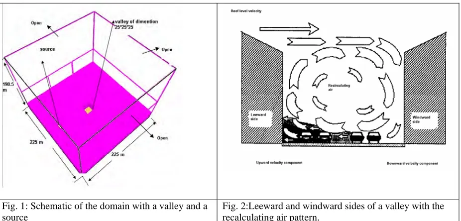
Fig. 1: Schematic of the domain with a valley and a source
Flow Pattern for a Cavity in Cross Flow:
For first study the schematic of a cavity in cross flow for a dense gas dispersion is shown in figure 1 and 5 different cases have been analysed. Initial wind velocity is kept 2.5 m/sec, except for the case with inlet velocity 1m/sec (here initial velocity has been taken as 0 m/sec). Plug velocity profile have been applied from left face of the domain (differs in each case) as shown in the figure 1. Rest all the faces of the domain are open except the bottom below valley. The figure 3 and 4 depicts the typical flow recirculation profile for two cases.
Fig. 3: Wind 3 m/sec flow pattern Fig. 4: Wind 5 m/sec flow pattern.
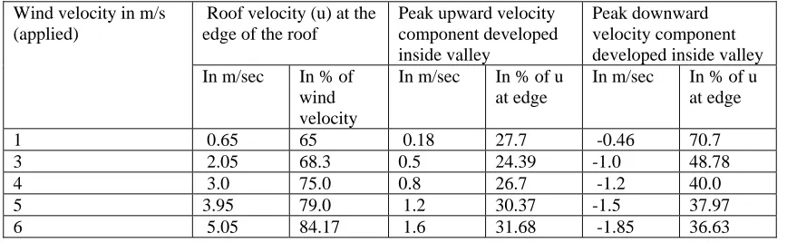
After post processing the results from all the following important observations were noted. Depending on the applied velocity which is a horizontal velocity in above case, a velocity component develops inside the valley. We can see the recirculation patterns development inside the valley due to applied horizontal component. The upward velocity component developed inside due to applied velocity is generally below 30% in magnitude of the u at the edge of the valley. The table 1 summaries the important finding of the present study.
Table 1: Summary of results for upwards and downwards velocity generation in a cavity in cross flow
Roof velocity (u) at the edge of the roof
Peak upward velocity component developed inside valley
Peak downward velocity component developed inside valley Wind velocity in m/s
(applied)
In m/sec In % of wind velocity
In m/sec In % of u at edge
In m/sec In % of u at edge
1 0.65 65 0.18 27.7 -0.46 70.7
3 2.05 68.3 0.5 24.39 -1.0 48.78
4 3.0 75.0 0.8 26.7 -1.2 40.0
5 3.95 79.0 1.2 30.37 -1.5 37.97
6 5.05 84.17 1.6 31.68 -1.85 36.63
Dense Gas Dispersion in a Cavity
For second study the schematic of a cavity in cross flow for a dense gas dispersion is shown in figure 1 and the table 2 depicts the various cases for parametric variation in dense gas source location and height. Initial velocity 0 m/sec for all cases, applied cross flow of 2 m/sec for all the cases along with a pollutant (SF6, atomic weight 140.12 amu) injection period is from 48 to 250 sec has been used in the simulation. The figure 5 and 6 depicts the typical concentration transient for two cases.
Table 2: Parametric variation for scalar injection source at cross flow before the cavity
Source geometry and location Case
Distance of injection source (m)
Height of injection source (m)
1. 50 29
3. 25 29
4. 50 33
5. 75 33
6. 25 33 met
7. 50 37 met
8. 75 37 met
9. 25 37 met
Fig. 5: Source at a distance of 50 meters from the valley and injection height 29 meters from ground level
Fig. 6: Source at a distance of 50 meters from the valley and injection height 33 meters from ground level.
After post processing the results from all the following important observations were noted. If the source is close to the valley the concentration of the pollutant will increase drastically. Also as the source distance increases from the valley there is higher time lag (proportional to the distance between source and valley) in pollutant concentration to built-up in the valley. If the source is close to the valley the pollutant accumulation will be more and the pollutant will remain with high concentration for a longer period despite of the fact that there is no more injection of the pollutant.
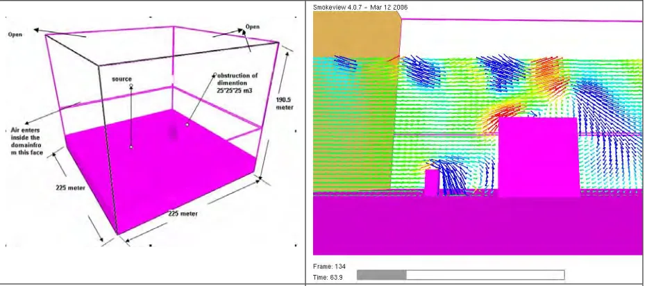
Flow Pattern for a Obstacle in Cross Flow
Initial velocity 0 m/sec for all cases with applied velocity 2 m/sec and a continuous injection of the pollutant (SF6, atomic weight 140.12 amu) after 48 seconds. Each side of the building is at a distance of 100 meters from corresponding parallel sides of the domain. Injection height (33 meter) and source dimensions along with its location in the domain are same for all the cases (Figure 7 and case a).
building.
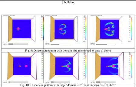
Fig. 9: Dispersion pattern with domain size mentioned as case a) above
Fig. 10: Dispersion pattern with larger domain size mentioned as case b) above
We can compare the case of vortex shading for the above mentioned two cases. In case (a) with smaller domain size the dispersion pattern seems to be mirror image due to small domain size with boundary conditions defined as open faces. This problem is eliminated by defining a domain of bigger size in case (b). Due to vortex shedding there is generation of some localized areas of higher concentrations.The edge facing the wind flow i.e. the front side of the building and the source have higher magnitude of the upward velocity component whereas the faces opposite to it have higher magnitude of the downward velocity component. Due to change in the wind blow pattern behaviour in presence of the obstructions some localized low velocity regions are also created.
COMPARISON OF POLLUTANT DISPERSION PATTERN: COMPLEX TERRAIN
For the sake of comparison the dispersion pattern of the pollutant has been shown below for three cases. Initial and boundary conditions are same for all the three cases: a)Dispersion of pollutant in a simple terrain; b) Dispersion of pollutant in a depression (cavity);c) Dispersion of pollutant in presence of a bluff body.
Fig. 11: Comparison of pollutant dispersion pattern: complex terrain
The following can be seen in this study. Maximum level of concentration at a particular time is highest for the case of complex terrain with a depression/cavity. Speed of travel of pollutant is highest in case of a simple terrain. High concentration band width along the vertical near to the ground is highest in case of a simple terrain. Pollutant concentration level beyond the obstructions is least in case of complex terrain with cavity. This phenomenon can be utilized for reduction in concentration of the heavy pollutant. But this cannot be said when there is a continuous release.
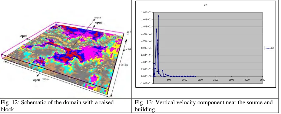
The CFD tool has been utilized to carry out the dispersion of tracer gas (SF6) at the Kaiga nuclear power plant (NPP) site. The computations were performed with the actual topographical data as shown in Fig. 12. The constant wind condition (Initial velocity: U0=2.75, V0=0.49 and velocity boundary conditions: Unormal=-2.71, Utangential=-0.67) have been applied. The Kaiga region topology is highly complex due to the presence of hills and river. The computational domain was 30000m (length) X 30000m (width) x 1500m (height). The source is released from 20000m, 20000m and 50m (height) from the left bottom corner. Total number of grids used in the simulation was 4.32 lakhs cells. The right side boundary was modeled as inlet where the available wind velocity was applied. The actual velocity was available at every 15 minutes. The SF6 was released at a rate as shown in Fig. 13 for a design basis accident of loss of coolant accident determined by another nuclear thermal hydraulic code RELAP and used in the present analysis as a time dependent boundary condition. Simulation started with 200 seconds delay to generate the wind field due to the modeled geometry. Simulation was performed for 6 hours. To understand the effect of actual topology Vis a Vis simple terrain computations (Gaussian plume equivalent computations), same computation has been revised by removing the topology obstruction data.
g/s
-2.00E+01 0.00E+00 2.00E+01 4.00E+01 6.00E+01 8.00E+01 1.00E+02 1.20E+02 1.40E+02 1.60E+02 1.80E+02
0 500 1000 1500 2000 2500 3000 3500
g/s
Fig. 12: Schematic of the domain with a raised block
Fig. 13: Vertical velocity component near the source and building.
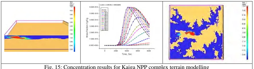
A typical study has been carried out to demonstrate the utility of the CFD code in the application for NPPs. Following salient conclusion have been brought out. Complex topography plays a dominant role in atmospheric dispersion of pollutant which is a function of space coordinates, time, wind velocity etc. Comparing Fig. 14 with Fig. 15 it is clear that the simple terrain assumption gives higher concentration at lower height at hill space where the pollutant actually should not exist in actual conditions and at high altitude it shows no scalars (where it should have significant values). Adjoining valley and hill regions also depicts entirely different atmospheric dispersion pattern. Comparison of the graphs for one typical receptors shows some interesting observation (Fig 14 and Fig 15).
Fig. 15: Concentration results for Kaiga NPP complex terrain modelling
The peak concentration at near to ground and at higher altitude can not be compared (in fact kind of inversion in trends exists). For the remaining mid range values the peak concentration observed with complex terrain are less as compared to simple terrain. Also there is a spread in the “time to reach peak concentration” values in complex terrain case due to enhanced mixing of scalar. Presence of complex terrain results in the increase in the “fall time” (from peak to insignificant values) values again due to enhanced mixing. Fig. 14 and 15 show the comparison of pollutant concentration for simple and complex terrain at specified height at various times. From these figures it is clear that dispersion is altogether different in complex terrain as compared to simple terrain Hence the dispersion modeling of complex terrain by adding obstructions of approximate size to a simple terrain will predict the dispersion behaviour that is not accurate. CFD based methods could be a versatile tool which can be used to handle most of the complex situations covering various scales.
CONCLUSION
Obstructions play a dominant role in atmospheric dispersion of pollutant which is a function of space coordinates, time, wind velocity etc. With increasing height, the pollutant disperses faster (by the study of changing concentration with elevation). There is a time lag in pollutant concentration built-up with increased number of obstructions on the path. Comparison of the graphs for specified locations show concentration built up at an elevation of 550 meter in between 1000 seconds to 1400 seconds (approx). Presence of complex terrain results in the fall in the pollutant concentration also. The comparison of the graphs for certain locations justifies that presence of complex terrain diverts the wind blow direction hence the pollutant transport behaviour of the atmospheric air is affected. Graphs for the few loactions project the behaviour of the dispersion with the changing heights of the obstructions in a complex terrain. As at certain elevations (say 0 meter and 650 meters etc) there is a large fluctuation in the pollutant concentration in presence of the complex terrain. There is a huge change in the concentration level of the pollutant on a plane (away from the source) a property which depends strictly on tin obstructions geometry. Hence the dispersion modelling of complex terrain by adding obstructions of approximate size to a simple terrain will predict the dispersion behaviour that is not accurate.
REFERENCES.
[1] J. S. Turner, “Proposed pragmatic methods for estimating plume rise and plume penetration through atmospheric layers”, Atmospheric Environment, vol. 19, pp. 1215–1218, 1985.
[2] R. B. Wilson, “Review of development and application of CRSTER and MPTER models”, Atmospheric Environment, vol. 27, pp. 41–57, 1993.
[3] F. Pasquill and F. B. Smith, Atmospheric Diffusion, 3rd edition, John Wiley, 1983.
[4] S. Hanna, “Review of atmospheric diffusion models for regulatory purposes”, World Meteorological Organization Tech. Rept. No. 581 Geneva, Switzerland pp. 44, 1982.
[5] D. B. Turner, Workbook of Atmospheric Dispersion Estimates: an Introduction to Dispersion Modeling. 2nd Ed. Boca Raton: Lewis Publishers of CRC Press, 1994.
[6] A. Venkatram and J. C. Wyngaard, Lectures on Air Pollution Modeling, Boston, American Meteorological Society, 1988.
[7] US Environmental Protection Agency, User’s Guide for the Industrial Source Complex (ISC3) Dispersion Models, Vol. II – Description and Model Algorithms, Publication EPA-454/B-95-003b, 1995.
[8] D. C. DiCristogara, S. R. Hanna, OCD: The Offshore and Coastal Dispersion Model, Volume 1: User’s Guide, Sigma Research Corporation, Westford, MA, Report No. A085, 1989.
[10] Akira Mori, “Integration of plume and puff diffusion models/application of CFD”, Atmospheric Environment, vol. 34, pp. 45-49, 2000.
[11] P. K. Sharma, S. G. Markandeya, A. K. Ghosh and H. S. Kushwaha, “Approaches for modelling of dispersion of pollutants in atmosphere with emphasis on computational fluid dynamics”, Proceedings of the NEHU, Shillong, 2004.
[12] P. K. Sharma, B. Ghosh, A. K. Ghosh and H.S. Kushwaha, “Analytical and computational fluid dynamics simulation for atmospheric dispersion in a large simple terrain of narora atomic power plant – a predictive calculation”, Proceedings of the 12th Annual Conference of Gwalior Academy of Mathematical Sciences (GAMS) and All India Symposium on Computational Biology, Maulana Azad National Institute of Technology, Bhopal, 2007.
[13] B. Gera, P. K. Sharma, R. K. Singh, A. K. Ghosh and H. S. Kushwaha “Approaches for modelling of atmospheric dispersion with emphasis on computational fluid dynamics and application of CFD for atmospheric dispersion in a large complex terrain of Kaiga atomic power plant”, Proceedings of the International Conference on Reliability, Safety & Quality Engineering, ICRSQE-2008, NPCIL, Mumbai, 2008.
[14] P. K. Sharma, B. Gera, A. K. Ghosh and H. S. Kushwaha, “Modelling of atmospheric dispersion in a flat terrain of Kakarapara atomic power plant (KAPP) including effect of building component”, Proceedings of the 36th National Conference on Fluid Mechanics and Fluid Power, College of Engineering, Pune, 2009.